Investigating Granular Structure with Spatial and Temporal Methods.

(1)

Abstract

OWENS, ELI THOMAS. Investigating Granular Structure with Spatial and Temporal Methods. (Under the direction of Karen E. Daniels.)

(2)

c

(3)

Investigating Granular Structure with Spatial and Temporal Methods

by

Eli Thomas Owens

A dissertation submitted to the Graduate Faculty of North Carolina State University

in partial fulfillment of the requirements for the Degree of

Doctor of Philosophy

Physics

Raleigh, North Carolina

2012

APPROVED BY:

Michael Shearer Keith Weninger

Jacqueline Krim Karen E. Daniels

(4)

Dedication

(5)

Biography

(6)

Acknowledgements

There are many people who I would like to thank and acknowledge for their help and support:

My adviser, Karen Daniels, for all your guidance and enthusiasm for my research

My Collaborators, Danielle Bassett and Mason Porter, for all your work and insight on

the network methods

Carl Schreck and Corey O’Hern, for your help and insight on the granular density of states

My fellow graduate students, James Puckett, Carlos Ortiz, Stephen Strickland, and Lake

Bookman, for sharing in the joys and struggles of graduate school

North Carolina State University, Physics Department. Thank you for accepting me into

the program and all the support.

The National Science Foundation for supporting this work

My parents, for always being there for me since my first breath.

The personal Creator and Sustainer of the universe, who has been a source of strength and

(7)

List of Tables

(10)

List of Figures

Figure 1.1 Hertzian contact diagram . . . 3

Figure 1.2 Force chains . . . 4

Figure 1.3 Granular force distribution . . . 5

Figure 1.4 Frictionless simulation of D(ω) . . . 13

Figure 1.5 Frictional simulation of D(ω) . . . 14

Figure 1.6 Network diagnostics . . . 22

Figure 2.1 Experimental setup . . . 27

Figure 2.2 Piezoelectric buffer circuit . . . 29

Figure 2.3 Schematic of the polariscope . . . 34

Figure 2.4 Schematic of photoelastic particle and contact forces . . . 35

Figure 2.5 High resolution static granular images . . . 36

Figure 2.6 Circle centers found from Hough algorithm . . . 37

Figure 2.7 Force fitting images . . . 38

Figure 2.8 Driver schematic . . . 40

Figure 2.9 Driver spectrum . . . 41

Figure 2.10 Piezoelectric time series . . . 43

Figure 2.11 Dynamic modulus . . . 47

Figure 2.12 Frequency dependent sound speed . . . 48

Figure 3.1 Experimental setup and camera stills . . . 55

Figure 3.2 Sample acoustic signal and amplitude decay with distance . . . . 57

Figure 3.3 Measured contact force and amplitude linearity . . . 60

Figure 3.4 Transient force chains . . . 61

Figure 3.5 Sound amplitude versus force . . . 63

Figure 3.6 Sound speed versus force . . . 65

Figure 4.1 Experimental setup and force chain images at different pressures 73 Figure 4.2 Sound attenuation in the bulk . . . 76

Figure 4.3 Velocity distributions . . . 79

Figure 4.4 Sample velocity autocorrelation function . . . 80

Figure 4.5 Density of modes and fc . . . 82

Figure 5.1 Sample force network . . . 89

Figure 5.2 Rattlers and (z-3) versus pressure . . . 94

Figure 5.3 Force chain and community images at different pressures . . . . 95

Figure 5.4 Adjacency matrix . . . 97

(11)

Figure 5.6 Number of communities as a function of Nγ . . . 99

(12)

Chapter

1 Introduction

(13)

results presented in this dissertation.

1.1 Granular Materials

Granular materials are composed of a collection of macroscopic particles that interact through a strictly repulsive potential that is present at the particle contacts. Granular materials differ in significant ways from ordinary solids, liquids, and gases. In fact, granular materials can act like all three phases of matter. For instance, walking on the beach the sand acts like a solid, whereas in an hour glass the sand pours and acts like a liquid, and in a sandstorm it acts like a gas [39].

Granular materials are a very common class of materials with which we have much everyday experience, from the sand on the seashore to coal that is burned to make electricity to pouring our cereal, granular materials are everywhere. There are also many industrial applications of granular materials. For example, one particularly important application of granular physics is in the area of oil and mineral exploration, since the earth is covered by a granular material.

(14)



f

2a

f

R

Figure 1.1: This figure illustrates the basic geometry used in Hertzian contact theory.

f is the applied force, δis the particle deformation (overlap in simulations), R is the

particle radius, and ais half the contact width.

1.1.1 Hertzian Contact Theory

The normal force interaction between grains in a granular material is described by Hertzian contact theory. The Hertzian potential is strictly repulsive and has a force law given by [51, 43],

f =αδβ (1.1)

where f is the applied force, δis the particle deformation (or overlap in simulations),

α is a constant that depends on the particle geometry and material properties, and β

is a constant that depends only on the particle geometry. A schematic of two particles in contact is shown in Figure 1.1. In general, we are primarily interested in βsince

this will have the most impact on the properties studied in this dissertation. Two commonly used ideal values are β=3/2 for spheres andβ=1 for disks.

(15)

deformation can be written as

δ = a

2

R (1.2)

where R is the particle radius and a is the radius of the contact area for spheres and half the contact width for disks [43] (Figure 1.1). This equation is valid when

δ is small compared to R. The contact area can then be found in terms of δ or f by

relating Equation 1.2 with Equation 1.1, and acan be written in terms of the Hertzian exponent, β, as follows:

a∝ f21β (1.3)

Therefore, contact area increases with contact force, and the relation between contact area and contact force will be important to interpreting the results in Chapter 3.

(16)

1.1.2 Force Chains

One of the characteristics of granular materials is that they are, in general, disordered systems. This manifests itself in disordered particle positions and in a disordered internal force structure (see Figure 1.2). One measurement of this disordered force structure is that the particle contact forces are observed to exhibit a probability distribution with an approximately exponential tail [69, 87, 61] (see Figure 1.3). This means that there are many particles with weak forces and a few particles that carry the majority of the stress in the system.

These particle contact forces are connected together in what are known as force chains. We have visually observed these force chains in 2D granular materials through the use of photoelastic particles (Figure 1.2), which when viewed through crossed polarizers reveal the stresses in the material. In general, a photoelastic disc which is subjected to multiple contact forces produces a complex fringe pattern (see

(17)

tion 2.3.1). However, it is approximately true that bright particles are under a higher compression than darker particles. Photoelastic particles provide a means to quantita-tively access the particle contact forces via a method that fits the experimental image to an analytical image of the photoelastic fringe pattern [86, 85].

Visual inspection of the force chains reveals that the chains form an interconnected branching structure, with a form that appears very disordered and irregular. An additional observation about the force chain images is that these pictures resemble a network in which the particles comprise the nodes and force is transmitted along particle contacts. This idea of describing the internal force structure of the material as a network will be investigated in Chapter 5.

(18)

1.2 Granular Acoustics

Granular acoustics is an active area of interest in part because of the promise acoustics holds for the non-destructive investigation of granular materials. While there have been several attempts to formulate continuum models of sound propagation in granular materials, it remains poorly understood [30, 63, 64]. These effective medium models fail to quantitatively describe important features of the material, and in particular they fail to predict the low pressure scaling of the sound speed.

Effective medium theories use the Hertzian force law given in Equation 1.1 to pro-duce effective bulk and shear modulii which then correspond to pressure dependent sound speeds. The sound speed,c, in a material is predicted to scale as the square root of the stiffness, c ∝ √s, where the stiffness is given by s = d f_d

δ, and for the Hertzian

contact law this means that,

s ∝δβ−1 (1.4)

For spheres, the Hertzian exponent is given byβ=3/2 and so comparing Equation 1.1

and Equation 1.4, the sound speed should scale as c ∝ f16. An assumption is then made that the average force between particles increases uniformly with the external confining pressure, P, so that the sound speed scales with pressure as c ∝ P16. This bulk sound speed scaling implies an effective Young’s modulus, E, for the material since c = pE/ρ where ρ is the density of the material. Effective medium theory

(19)

and non-affine effects [30] and deviations from the ideal particle contact area [38].

1.2.1 Sound Propagation along a 1D Chain

Due to the heterogeneous structure of granular materials, there has been a great deal of difficulty in describing how the internal force structure of a granular packing affects its acoustic response. Simpler 1D chains of grains have been studied to help elucidate the role of interparticle forces on granular acoustics [71, 53]. These acoustic experiments on 1D granular chains can be divided into linear and non-linear sound propagation experiments. In the non-linear regime, the static force confining the chain is on the order or smaller than the dynamic force produced by the acoustic wave [72]. With a pulsed input, this non-linear sound propagation gives rise to solitary waves and the sound speed scales with the amplitude of the wave [82, 83, 18, 15].

In the linear regime, the sound amplitude is smaller than the confining force. As described earlier, the speed of sound is predicted to scale as c∝ f16, where f is now the force on the 1D chain. For a 1D chain, the pre-factor can also be found and the theoretical prediction of the sound speed in a 1D chain is given by Coste and Gilles [16],

c = √1

πρ

9E

2R(1−σ2)

1/3

f1/6 (1.5)

whereρis the material density,Eis the Young’s modulus, σis the Poisson ratio, and f

(20)

Hertzian exponent.

1.2.2 Granular Acoustics in 2D and 3D

There have also been many experiments on 2D and 3D granular packings. Liu and Nagel [56, 55, 58] performed granular acoustics experiments on a 3D packing of glass beads, and observed that there is no single sound speed in a granular material. They computed a time of flight sound speed using the familiar formula,c = ∆_∆x_t, where ∆x

is the distance from the source to the detector embedded inside the packing and∆tis the change in time from when the pulse was sent to when it was received. With this definition of speed, they observed that the speed of sound in the material depended on the particular way∆twas measured. They found that when∆t was found from the difference in time between the peak amplitude in the transmitted signal and the peak amplitude in the received signals the corresponding sound speed was slower than when∆t was found from the difference in time between when transmitted signal and received signals rose above the noise threshold. They also measured the group velocity and found it to be slower than either of the two time of flight speeds defined above. This curious phenomenon, that the time of flight sound speed depends on the particular definition of ∆t, has also been observed in simulations [94]. In Chapter 3, we also observe this effect and are able to explain it as arising from the sound being able to arrive at a location via multiple paths through the system.

(21)

Similar inferences to the effect of force chains where made by Hostler and Brennen [36] when they saw that loose unconsolidated packings had inconsistent acoustic responses, which they also attributed to rearrangements in the force network. From these experimental observations, the importance of force chains was hypothesized; however, no direct observations of the force chain network were made [57, 55, 36].

The above experiments suggest that the underlying force network in a granular material plays a crucial role in sound propagation. However, experiments have not been able to directly measure the effect force chains have on sound propagation, and have only inferred its importance. These inferences about the importance of force chains in granular acoustics are at odds with simulations done by Somfai et al. [94] in which they did not find the force chains to significantly influence granular sound propagation. In the work presented in this dissertation, we are able to directly observe the force chains and the dynamics along them through our use of photoelastic particles. In Chapter 3, we will use this ability to experimentally measure the force chains and directly test the role of inter-particle forces in sound propagation through a 2D granular material.

1.3 Jamming and Vibrational Modes

(22)

jamming in experimental granular materials, our results are relevant regardless of the applicability of jamming to granular materials.

Jamming occurs for a loose granular packing when the packing is compressed sufficiently to become able to support a finite pressure. How much a packing is compressed is commonly measured in terms of packing fraction,φ, which is defined

as

φ= Vpart

Vsys (1.6)

where Vpartis the total volume of all the particles and Vsys is the total system volume. The point at which the material is first able to support a pressure occurs at a packing fraction φc and is known as the jamming transition [97, 54, 107]. The jamming transition can also be described in terms of the average number of particle contacts, z. As the pressure is increased, the number of contacts also increases, and at some value of average contact number,zc, the system jams.

For the system to be rigid, each particle must have all of its degrees of freedom, B, constrained by its adjacent particle contacts. If each contact has Fforce components, then for a particle to be constrained the following relation must be satisfied: zF₂ ≥B. Frictional particles in 2D have 3 degrees of freedom, two translational and one rotational, and the particle contacts each have 2 force components. Therefore, the minimum number of contacts to constrain frictional 2D spheres or discs is zc = 3. Relations forzc have also been developed to describe ellipsoidal particles [2, 97].

The jamming transition can also be described in terms of the density of states,

D(ω), where simulations and measurements have shown that granular materials

(23)

These soft modes are associated with a loss of mechanical rigidity as the jamming transition is approached and the system unjams.

1.3.1 Simulations

The density of states, D(ω), is a concept borrowed from thermal physics and relates

the number of vibrational modes available to the system at a given frequency, ω. Since

granular materials are composed of macroscopic particles that do not have thermal vibrations, a granular D(ω) is not strictly valid. However, a quantity analogous to

D(ω) can be found for a simulated granular packing using the particle positions and

the interaction potential,V. In the linear approximation, the interaction potential is given by [3],

V = 1

2u

†_Ku _(1.7)

where uis the vector displacement of the particles and K is the Hessian or stiffness matrix. The elements of the dynamical matrix,D, of the system are then defined as,

Dij = 1 mi

∂2V ∂ui∂uj

= Kij

mi (1.8)

where mi is the mass of particle i. This dynamical matrix can be thought of con-ceptually as being related to a matrix of spring constants, and the eigenvalues of the dynamical matrix correspond to the square of the system’s vibrational modes. Therefore, computation of a dynamical matrix provides a means to find D(ω) for

(24)

10−2 10−1 100 101

ω

10−2 10−1 100 101

D(

ω

)

(a)

10−6₁₀−5₁₀−4₁₀−3₁₀−2₁₀−1 ₁₀0

φ−φ

_c 10−3 10−2 10−1 100 101

ω

* (b)

Figure 1.4: (a) Shows the density of states for a simulated frictionless granular material for several different packing fractions. (b)ω∗ as a function of distance from

the jamming transition φ−φc. The solid line shows ω∗ ∝ (φ−φc)1/2. Reprinted figures with permission from Silbert et al. [92]. Copyright (2005) by the American Physical Society1. http://prl.aps.org/abstract/PRL/v95/i9/e098301

the vibrational energy of the system is no longer described by the eigenvalues of the dynamical matrix, and the vibrational energy becomes smeared out over a continuous band of frequencies. Very far from the linear approximation, the energy shifts to lower and lower frequencies.

Using this dynamical matrix method, D(ω)has been calculated for simulations of

frictionless granular materials [76, 92, 106, 93, 112, 60]. In simulations of frictionless spheres, D(ω) of the granular material is compared to the Debye prediction for D(ω)

in crystalline materials. The Debye scaling predicts that at low frequencyD(ω) ∝ωd−1

wheredis the dimension of the system. It is observed that the granularD(ω) deviates

from this low frequency prediction and has an excess number of low frequency modes which increase as as the system approaches the unjamming transition (see Figure 1.4a).

1_{Readers may view, browse, and/or download material for temporary copying purposes only,}

(25)

Figure 1.5: Result of computing the density of states for a frictional granular simulation. (a) ω∗ as a function of system pressure, P, for several different friction coefficients.

(b) ω∗versusz−3 showing that the data collapses for this scaling. Reprinted figures

with permission from Somfai et al. [95]. Copyright (2007) by the American Physical Society2. http://pre.aps.org/abstract/PRE/v75/i2/e020301

This deviation is quantified with the introduction of a critical frequency ω∗ which

can be defined as the frequency above whichD(ω)deviates from the Debye scaling.

The critical frequency ω∗ was seen to scale a function of distance from the jamming

transition as ω∗ ∝(φ−φc) 1

2 [97, 54] as shown in Figure 1.4b.

There are also simulations of frictional granular materials [95, 32] from which

D(ω) is calculated, and an excess of low frequency modes is also observed. The

critical frequencyω∗ can again be defined and used to quantify how the excess modes

scale with pressure(ω∗ ∝ Pγ). However, the scaling relation betweenω∗ and pressure

depends strongly on the coefficient of friction (see Figure 1.5). Work by Somfai et al. 2_{Readers may view, browse, and/or download material for temporary copying purposes only,}

(26)

[95], simulated a granular packing using friction coefficients ranging from 0.1−10 and found that except for the very highest values of the coefficient of friction, the relation

ω∗ ∝ Pγ is very flat. If instead, the relationship betweenω∗ andz−3 is investigated,

a universal scaling relation is found that does not depend on the coefficient of friction. The relation is ω∗ ∝(z−3) suggesting the importance of contact number, rather than

pressure as in frictionless materials, in describing the jamming transition and rigidity of the material.

1.3.2 Experiments

While using the dynamical matrix is a useful technique for simulations, it is not experimentally feasible to find D(ω) using the dynamic matrix approach since the

interaction potential and particle positions are rarely known with sufficient resolution. Therefore, other methods have been developed to measure D(ω) in experimental

systems. In experiments on colloids [26, 12, 46, 13, 28, 27, 111] and on a laboratory granular material [9], a covariance matrix method [33] was implemented to find D(ω).

The elements of the covariance matrix, Care given by

Cij =hui(t)uj(t)i (1.9)

whereui is the displacement of particleiaround its equilibrium position and uj is the displacement of particle jaround its equilibrium position andh·idenotes an average over time. It can be shown [33], that the covariance matrix for thermal materials is related to the dynamical matrix as follows:

C= kBTD

−1

(27)

where m is the particle mass, kB is the Boltzmann constant, T is the temperature, and D−1 is the inverse of the dynamical matrix. It is apparent from Equation 1.10, that the eigenvalues of the covariance matrix are proportional to the inverse square of the vibrational modes of the system. In colloidal experiments, the particles have thermal vibrations which produce particle displacements, and so Ccan be found by tracking the particles as they vibrate. Then D(ω) can be found from the covariance

matrix. This procedure does not find the true density of states for the system since the particle motion is damped by the fluid in which the colloidal particles are suspended.

D(ω) is instead the density of states for a shadow system that does not have the

damping which is present in the experimental colloidal material. This colloidal D(ω)

also shows the excess long wavelength soft modes seen in the simulations of granular materials [26, 12].

The covariance method has also been employed in an experiment on a granular material [9]. Since unlike colloids, granular materials do not have any thermal motion. The granular material had to be vibrated to produce particle motion that could be tracked to produce the covariance matrix. Since these experiments rely on mechanical vibrations to thermalize the system, Brito et al. [9] checked how well the system had been thermalized by looking at the particle displacement distributions. These distributions showed that for low amplitude vibrations and short measurement times the displacement distributions were Gaussian and caged around an average position. However, the width of these distributions was found to vary from particle to particle even for particles from the same packing. This highlights an important deviation from a true thermal system. However, they were still able to measure a D(ω) and find

(28)

While this covariance method is a very powerful tool, it does have some shortcom-ings. In particular, the positions of all the particles in the system must be tracked to find their displacements and compute the covariance matrix. This necessitates the use of specialized packings where there is optical access to the particles. Also, the resolution of the final result is limited by the resolution of the camera used to track the particles. It would therefore be beneficial to have a method to computeD(ω)in a

real granular system where there is no optical access.

1.3.3 D

(

ω

)

through the Spectrum of the Velocity Autocorrelation

The two methods that have been used to find D(ω) in granular materials are the

dynamical matrix method which is used with simulations and the covariance matrix method which has been used on an experimental granular packing. In this section, we present a third method that will be adapted in Chapter 4 and used to find D(ω) in

an experimental granular packing. This third method is taken from thermal physics where the spectrum of the velocity autocorrelation function [19, 47] is commonly used to find D(ω), as it has been shown that the spectrum of the velocity autocorrelation is

equivalent to D(ω). Below, I present a brief derivation of this method and highlight

some important assumptions 3. In order to derive this relation, first start with the displacement, uj, of particle jgiven by,

uj(t) = ΣkAkj(t)eiωkteˆk (1.11) 3_{Thanks to Carl Schreck and Corey O’Hern (Yale) for personal communications which were}

(29)

where, Akj is the amplitude of particle j0s kth mode, ωk is the frequency of the kth mode,t is time, and ˆek is thekth eigenvector. The velocity, vj(t), of particle j is then given by,

vj(t) = ΣkiωkAkj(t)eiωkteˆk (1.12)

From here, we can define the unnormalized velocity autocorrelation function,Cv0(t),

C_v0(t) =

∑

j

hvj(τ+t)·v∗j(τ)iτ (1.13)

where τ is some reference time. Now we make our first assumption, which is that

dissipation is small and the particles are in a steady-state regime. Therefore, they vibrate with the same average amplitudes at all times and so Aki(τ+t) = Aki(τ). Using this assumption,

hvj(τ+t)·v∗j(τ)iτ =Σklh(iωkAkj(τ+t)eiωk(τ+t)eˆk)·(−iωlAlj(τ)e−iωlτeˆl)i

=Σ_khAkj(τ+t)Akj(t)ω2_kieiωkt

=Σ_khAkj(τ)2ω2kieiωkt

(1.14)

We now make our second assumption which is that the equipartition theorem holds. This means that 1₂mhA2_kω2_kiτ =kBT where A2_k =ΣjA2_kj. Using this assumption,

Cv0(t) = ΣjΣkhAkj(τ)2ωk2ieiωkt

=Σ_khΣ_jAkj(τ)2ωk2ieiωkt

=Σ_khAk(τ)2ω2_kieiωkt

= 2kBT

m Σke iωkt

(30)

Now we take the Fourier transform ofC_v0(t),

Z ∞ −∞C

0

v(t)e−iωktdt = 2kBT

m Σk

Z ∞ −∞e

−i(ω−ωk)t_dt

= 2kBT

m Σkδ(ω−ωk)

(1.16)

This equation can then be compared to the density of states given by,

D(ω) = Σkδ(ω−ωk)

Nk

(1.17)

where Nk is the total number of vibrational modes and is equal to Nk = ₂_km_B_T ·C0v(0). The density of states then can be written as,

D(ω) =

Z ∞ −∞

C_v0(t)

C_v0(0)e

−iωkt_dt ₌ Z ∞

−∞Cv(t)e

−iωkt_dt _(1.18)

WhereCv(t) is given by,

Cv(t) =

∑jhvj(τ+t)·v∗j(τ)iτ

∑jhvj(τ)·v∗j(τ)iτ

(1.19)

Therefore, the spectrum ofCv(t) is equivalent to D(ω) and can provide an alternative

technique for measuringD(ω)if particle velocity information is available. In Chapter 4,

(31)

1.4 Networks

Another way that granular materials can be characterized is with a network approach, which seems to be an intuitive approach based on inspection of images of the force network, such as Figure 1.2. Network theory has been an area of great interest and study, and it has been applied to a multitude of problems [75] ranging from the spread of disease [67], the internet [23], ecosystems [11], and many other areas. In its simplest form, a network is a collection of elements (nodes) that are related to each other in a particular way. If two nodes have a relationship between them, then the nodes are connected by an edge. For example, in the network of airports, airports comprise the nodes of the network and there is an edge between airports which have flights between them.

In order to perform operations on networks, it is necessary to be able to represent the network mathematically. This is accomplished with an adjacency matrix,A. In its most basic form, Aij = 1 when nodei is connected to node jand Aij =0 when the nodes i and j are not connected. Another more descriptive adjacency matrix is the weighted adjacency matrix, W, in which the element Wij is equal to some measure of the strength of the interaction between nodes, for instance the number of flights between airports in the airport network.

(32)

particular geographic location in space, for instance the grains in a granular network or airports in the airport network are located at specific locations in space.

Network methods have previously been applied to granular materials by several researchers [101, 34, 100, 6]. Experiments on a sheared granular system [34, 100] examined a broken link network; the adjacency matrix elements conveyed what particles which had previously been in contact had their contacts broken. This approach enables them to relate a network diagnostic (clustering coefficient) to the number of broken edges.

Network techniques have also been applied to simulated granular materials [101, 100]. These simulated granular materials were bi-axially compressed and a variety of network diagnostics were tested to try and characterize the material as it was compressed. Numerous network diagnostics were investigated for both weighted and binary contact networks, and in particular, it was found that the network could be partitioned into three subgroups. Walker and Tordesillas [100] found that particles within a given subgroup had similar properties, and the three subgroups corresponded to particles in the shear band, force chain particles, and non-force chain particles respectively.

In collaboration with Danielle Bassett and Mason Porter, we have tested of a broad range of network diagnostics on an experimental granular packing [6]. We surveyed many network measures and rated the reliability of each diagnostic through the use of a reliability coefficient; Reference [6] contains a full listing and description of the diagnostics we used.

(33)

0

500

1000

800 1000 1200 1400

0 0.₅ 1 x 10

−3

0

500

1000

800 1000 1200 1400

0 0.₅ 1 x 10

−3

0

500

1000

800 1000 1200 1400

0 0.₅ 1 x 10

−3

0

500

1000

800 1000 1200 1400

0 0.

5 1 x 10

−3

0 1x10-3

global efficiencyEw log (X (z+5))

2

community structure

Bw

geodesic node betweenness clustering coefficientCw

0.6 2.2

0 7x104 0 200

A

B

C

D

0 500 1000

−1400 −1200 −1000 −800 −600 −400 −200

0 500 1000

−1400 −1200 −1000 −800 −600 −400 −200

0 500 1000

−1400 −1200 −1000 −800 −600 −400 −200

0 500 1000

−1400 −1200 −1000 −800 −600 −400 −200

0 500 1000

−1400 −1200 −1000 −800 −600 −400 −200

0 500 1000

−1400 −1200 −1000 −800 −600 −400 −200

0 500 1000

−1400 −1200 −1000 −800 −600 −400 −200

0 500 1000

−1400 −1200 −1000 −800 −600 −400 −200

0 500 1000

−1400 −1200 −1000 −800 −600 −400 −200

0 500 1000

−1400 −1200 −1000 −800 −600 −400 −200

0 500 1000

−1400 −1200 −1000 −800 −600 −400 −200

0 500 1000

−1400 −1200 −1000 −800 −600 −400 −200

0 500 1000

−1400 −1200 −1000 −800 −600 −400 −200

0 500 1000

−1400 −1200 −1000 −800 −600 −400 −200

0 500 1000

−1400 −1200 −1000 −800 −600 −400 −200

0 500 1000

−1400 −1200 −1000 −800 −600 −400 −200 10

(34)

geodesic node betweenness [81, 73] is sensitive to 1D chains of nodes (force chains), (iii) clustering coefficient [4] is sensitive to the particle scale, and (iv) modularity [84, 74, 24] is sensitive to intermediate meso-scale features.

One of the goals of this study was to try and correlate sound propagation with a network measure, and we found that network modularity was descriptive of the sound propagation. Modularity divides the network into sub-regions or communities. These communities represent collections of highly connected nodes, and we found that a particle’s connectedness to its own community could be correlated to both the force on it and to the amplitude of sound through the particle.

Application of network tools to granular materials holds much promise. Since different diagnostics are sensitive to different dimensionalities of the system, particular size scales can be probed by selecting an appropriate network diagnostic. In Chapter 5, we will use network modularity to probes intermediate length scales in the system. We will test whether such a length scale may be able to describe the system’s distance from the jamming transition either by a changing size or a changing community shape with pressure. We find that the shape becomes more circular as the pressure is increased, but the size of the communities remains constant with pressure.

1.5 Overview of Experiments

(35)

measure the particle contact forces. Inspired by methods used to measure sound in a 1D granular chain [18], we use piezoelectric sensors embedded inside individual particles to measure the sound at the particles scale. These particle scale acoustic measurements are combined with the use of photoelastic particles in which we can resolve the static particle positions and force chains. These two basic measurement techniques allow us to investigate a variety of problems related to how disorder in both particle positions and inter particle contact forces influences spatial and temporal granular material properties.

In Chapter 3, we study how the force chains effect sound propagation in the linear sound propagation regime. Combining particle scale sensors and high speed imaging of the photoelastic particles, we are able to image sound propagation through our granular packing, and we see that the sound travels preferentially along the force chain network. Quantifying this result, we see that the sound amplitude scales with the particle contact area, suggesting that the particle contact area provides the main conduit for sound propagation. We also observe two sound speeds in our material. The first sound speed is the speed of the leading edge of the signal. This speed corresponds to the sound which travels along the strongest force chains and therefore arrives first. The second sound speed is the speed of the peak response. This slower sound speed is a combination of waves that reach our sensors over multiple paths. This work shows the force chains to be an important component of sound propagation through a granular material.

(36)

autocorrelation function (see Equation 1.18) to find the density of modes. The response of the system is then observed with particle scale sensors embedded in the packing. The density of modes is found for both a disordered bi-disperse mixture of grains and a mono-disperse hexagonally ordered system, and for both systems the number of low frequency modes is seen to increase as system pressure is decreased. This is in qualitative agreement with the previous work done on the density of states. We also observe Debye scaling at the highest pressure in the ordered system. This further confirms the validity of our application of a thermal method to a granular system. The technique used for this novel measurement of the density of modes is highly versatile, and could easily be applied to 3D systems and/or to systems using non-spherical particles.

(37)

Chapter

2 Experimental Methods

(38)

driver

weight

g

piezoelectric

sensors

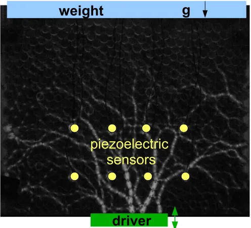
Figure 2.1: Basic setup used for experiments showing the brass weight used to vary the pressure, the electromagnetic driver is at the bottom of the system, and piezoelectric sensors distributed throughout the pack.

as in Chapters 4 and 5. An electromagnetic driver is fixed to the bottom of the system and is used to excite acoustic waves.

2.1 Piezoelectric Sensors

(39)

acoustic response at the grain scale.

Table 2.1 summarizes some of the piezoelectric sensors properties, and Figure 2.2 shows the circuit [45] used to amplify and buffer the piezoelectric signal. Buffering the signal is necessary since the piezoelectric element has a very high output impedance that must be reduced in order to correctly read the output voltage on the LabView DAQ card.

Table 2.1: Piezoelectric Properties

Property value

Manufacturer Piezo Systems

Part Number PSI-5A4E

Material Lead Zirconate Titanate Dielectric Constant,ε 1800

Thickness, d 2.03 mm

Surface Area, A 4×4 mm2

Cpiezo 0.13 nF

Cwire 16 pF

Ctotal 0.15nF

flow 106 Hz

d33 390×10−12 C/N

2.1.1 Piezoelectrics as Circuit Elements

The capacitance of the piezoelectric, Cpiezo, can be found using the simple parallel plate capacitor equation as follows:

Cpiezo =εε0A

(40)

+

- +

- Vout

R1

=

1

0

M

Ω

R₂ = 2 kΩ R₃ = 8 kΩ

TL071

Figure 2.2: The circuit used to buffer and amplify the piezoelectric sensors in Chapter 4. The circuit used in Chapter 3 does not include the non-inverting amplifier made by

R2or R3 and the op-amp. This circuit uses Texas Instruments TL071 op-amps.

Where εis the dielectric constant, ε0 is the permittivity of free space, Ais the surface

area of the piezoelectric, andd is the thickness of the piezoelectric.

The capacitance of the wires, Cwire, must also be found. The capacitance per foot of the wire can be found from the following equation for twisted pairs [10]:

Cwire

l =

2.2ε

ln(1.3_f_··_dD)

pF

ft (2.2)

Where l is the length of the wire in units of feet,εis the dielectric constant of the wire

insulation material,D is the outer diameter of the wire (over the insulation), dis the diameter of the conductor under the insulation, and f is the stranding factor which is related to the number of strands that make up the wire.

For our setup, the wires have PVC insulation. The dielectric constant for PVC ranges from approximately 3.5-6.5 and so we will use ε= 5. The outer diameter is

(41)

on the number of strands per wire and is found from the tables listed in Reference [10]. For our wires, there are 26 strands per wire and so f = 0.975. Using these values, the capacitance per foot of wire is C_l = 7.8 pF_ft, and the wires we use are 2 ft long so the total capacitance of the wires is Cwires = 16 pF. Finally, the total capacitance of the sensor can be found from capacitance of the piezoelectric in parallel with the capacitance of the wires,Ctotal =Cpiezo+Cwire =0.15 nF.

The total resistance, R, of the sensor is the combination of the internal resistance of the piezoelectric and the parallelR1=10 MΩ resistor put across the piezoelectric

before it goes into the op-amp as shown in Figure 2.2. The internal resistance of the piezoelectric element is much larger than 10 MΩ and so the total resistance of the sensor is just R =10 MΩ. The piezoelectric sensor then has a low frequency cutoff given by flow= ₂_π1_RC =106 Hz

2.1.2 Converting Voltage to Force

Piezoelectric elements produce a charge output,Q, that is proportional to the applied force, F, such that,

F= Q

d33 (2.3)

whered33 is the constant of proportionality and depends on the piezoelectric material

used. Our sensors are made of a particular type of lead zirconate titanate (PZT) piezoceramic for which the manufacturer lists d33 =390×10−12 C/N. In order to get

(42)

voltage and charge relationship in the circuit is given by:

V = Q

Ctotal

·G (2.4)

WhereG is the gain of the circuit and is set by the resistorsR2 and R3 in Figure 2.2.

These resistors and the op-amp make a non-inverting amplifier and soG =1+R3 R2. The circuit used in Chapter 3 did not include resistors R2 andR3and so the gain is 1 for

the experiments performed in Chapter 3. In Chapter 4, a 10 k, 20 turn, potentiometer was used for R2 and R3 allowing a gain of 5 to be set for all the sensors in Chapter 4.

Finally, the voltage to force conversion is given by

F =

0.385 N V

V

G (2.5)

2.2 Acoustic Exciters

In Chapters 3 and 4, acoustic excitations are used to probe the structure of the granular packing. We excite acoustic waves using electromagnetic drivers which operate on the voice coil principle. When current is passed through wire loops, a force is exerted on a permanent magnetic rod inside the wire loops. The force, F, is proportional to the current, I, and the magnet flux density, B, of the rod,

F =Bn`I (2.6)

(43)

All of the acoustic experiments are controlled by a LabView DAQ card, model PCI-6255. This card was used to control the driver as well as record the acoustic responses of the sensors. This card has two analog outputs with 16 bit resolution, and can read up to 40 channels differentially at 16 bit resolution. The sample rate of the card is 1.25 MS/s.

In different experiments, we have used one of two electromagnetic drivers to excite the acoustic waves. The main difference in the two acoustic sources is the maximum peak force available. The experiments in Chapter 3 used a small voice coil that produces a peak force of 6.7 N, but for the experiments in Chapter 4 we upgraded to a larger electromagnetic driver that can produce 220 N of peak force.

2.2.1 Voice Coil Driver

(44)

2.2.2 Electromagnetic Driver

For the experiments performed in Chapter 4, an electromagnetic driver was used to excite the white noise signals. It was manufactured by MB Dynamics and is their model PM50A vibration exciter. This driver provides a peak force of 220 N and has a maximum displacement of 13 mm. This much more powerful driver allowed us to compensate for its mechanical resonances. Due to its large size, this driver was supported on an isolation table manufactured by Kinetic Systems, Inc., model Vibraplane Model 9321-9327. The driver was controlled by a Yamaha power amplifier model PC3301N.

2.3 Pictures and Image Processing

(45)

incoming light

right circular

polarizer photoelasticmaterial left circularpolarizer camera

Figure 2.3: Schematic of the polariscope. The circular polarizers are made from the combination of a quarter wave plate and linear polarizer.

2.3.1 Photoelasticity

Photoelastic materials are a special class of materials that become birefringent under stress [25, 31]. Birefringence is an optical property in which the birefringent material has two indices of refraction. These two indices of refraction are along different directions in the material, and rotate the polarization of light that passes through the birefringent material. A photoelastic material only becomes birefringent under stress and so when unstressed has only one index of refraction. As such, if an ideal unstressed photoelastic material is placed between two crossed polarizers (see Figure 2.3) no light will be transmitted. However, if the photoelastic material is then stressed, the material will become birefringent and the polarization of the light will change allowing some light to make it through the crossed polarizers. The intensity, I, of the transmitted light at a given location is given by,

I =sin2π(σ1−σ2)

Fσ

(46)

Figure 2.4: This image shows a sample photoelastic particular viewed between two crossed circular polarizers. The particle has three contact forces at the locations indicated by the arrows.

where σ1 and σ2 are the principle stress components of the photoelastic material

and Fσ is the stress optic coefficient which is a property of a particular material and

geometry.

(47)

(a) (b)

Figure 2.5: Example of the two static images taken for each packing. (a) Image without the polarizers clearly showing the particle and piezoelectric sensor locations. (b) Image with the polarizers showing the force chains.

2.3.2 Finding Particle Centers and Contact Forces

Since the granular material is made of photoelastic disks, the internal forces can be seen when the material is viewed through crossed circular polarizers. In order to quantitatively measure these internal forces, we take two static images of all our packings. The first image (Figure 2.5a) is taken without the polarizers and is used to find the location of the particle centers via a Hough transform method [110], and a sample image showing the particle centers is shown in Figure 2.6. The second image is taken with polarizers and shows the force chains (Figure 2.5b) and is used with the particle centers to find the inter-particle contact forces.

(48)

Figure 2.6: Camera image of the particles, overlaid with the locations found with the Hough code [110].

since the embedding process freezes stress into the particles. We therefore give these particles their neighbor’s contact forces. We also re-assign particles with unrealistically high contact forces their neighbor’s force and remove contacts with very low forces since these are typically false contacts. As a final step, we average the contact forces between two particles so that Newton’s third law is preserved across the contact. This final processing of the contact forces gives a very nice fit to the image, and an example of this fit is shown in Figure 2.7c.

2.3.3 Cameras

(49)

(a)

(b) (a)

(c)

(50)

the ability to take pictures remotely, which greatly increased the consistency of our pictures since we did not have to touch the camera to take pictures.

2.4 White Noise Acoustic Excitations

In Chapter 4, we use a white noise acoustic signal, which has a flat spectrum, to excite the vibrational modes in the granular material. Producing such an input spectrum is not a trivial matter and requires that we compensate for the mechanical resonances of our driving apparatus. For this task, we used the large electromagnetic driver since the small voice coil would need to be driven with higher current than its maximum current rating allows.

2.4.1 The Input

(51)

dr iv er s ha ft driver head direction of motion piezo granular material stabalizer bar shaker

Figure 2.8: This figure illustrates the driver and how the piezoelectric sensor is mounted onto the driver and is isolated from the granular material.

˜

V0 =

      

f ·w˜ for f < fhigh

0 for f > fhigh

(2.8)

where f is the frequency and ˜w is a white noise signal generated by the computer. However, the shaker cannot supply power up to infinitely high frequencies, and so we use a low-pass filter to limit the input frequencies to less than fhigh.

For each individual packing, the driver sends in a test signal, given by equation 2.8, and the driver sensor measures the driver response, ˜Vdr, so that deviations from equation. 2.8 can be corrected. The driver response is then used to produce a corrected input, ˜V, given by,

˜

V = f ·V˜

0

˜

Vdr

(52)

102 103 104

frequency (Hz)

power

1/2

ordered

102 103

104

frequency (Hz)

power

1/2

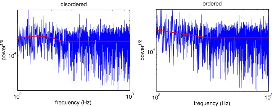
disordered

Figure 2.9: These figures show the power spectrum of the driver in response to driving the (a) disordered and (b) ordered systems. As can be seen, the low frequency part of the driver spectrum deviates from flat and the fit to the low frequency part of the spectrum is shown by the red curve.

A final critical step is to reapply our low-pass filter to the signal before transforming back to real space. The signal ˜V is now transformed back into real space giving a final input signal,V(t), used to drive the system for the experiments. Now that the correct input signal has been obtained, the driver can vibrate with a flat velocity spectrum up to fhigh, provided the amplitude is high enough to excite the lower frequencies. For the work presented in Chapter 4, fhigh =3000 Hz.

(53)

and allow us to extend our measurements down to 100 Hz.

2.4.2 Design Considerations

While the above protocol is effective at compensating for small mechanical resonances, it cannot compensate for very large resonances or insure that the vibrations are the same everywhere on the driver head. These remaining issues are solved by careful design and mounting of the driver. In our original experiments, we tried to use a driver head that was as wide as the whole bottom of the granular packing. However, when we monitored the response near the center of the driver and the response on the edge of the driver we found different driver responses. This was due to the fact that we could not make the driver head and driver shaft rigid enough and so there were additional vibrational modes introduced into the system. We compensated for this problem by using a smaller driver head. However, if one wanted to use a very wide driver head it would have to be very rigid, and the shaft from the shaker would have to have minimal free play to avoid rattling at high frequency.

It was also very important that the drive shaft be perfectly centered through the support shaft with minimal rubbing. For some of our early tests, this was not the case and it was nearly impossible to compensate for the mechanical resonances of the system.

2.4.3 Measuring the Response

(54)

0 1 2 3 −0.3

−0.2 −0.1 0 0.1 0.2 0.3

time (sec)

voltage

2 sec measurement

0.1 0.15

−0.2

0

0.2

time (sec)

voltage

2.88 2.92

−0.2

0

0.2

time (sec)

voltage

(55)

send in a white noise signal for 2.8 sec and then only use the middle 2 sec for our analysis (see Figure 2.10). This insures that we are not sampling the initial part of the signal as it builds up to steady state, or the last parts of the signal as it decays once the vibrations are turned off. We observe that the time needed to reach steady state and decay away are on the order of milliseconds and so the middle 2 sec are in the steady state regime.

2.5 Viscoelasticity

For all of our experiments, we used Vishay PSM-4 photostress material which is a viscoelastic material. Viscoelasticity is a common material property, and describes how the stress,σ, is related to the strain, e, of a material under a dynamic load. Viscoelastic

effects are dynamic effects [50] and will therefore be important to interpreting the results in Chapters 3 and 4, with the most important effects encountered being related to a frequency dependent Young’s modulus, sound speed, and sound attenuation.

2.5.1 Basic Properties

First, let us define some basic properties of a viscoelastic materials subjected to a sinusoidal stress driven at frequency, f. The stress as a function of time is given by,

σ(t) = σ0sin(2πf t) (2.10)

whereσ0 is the amplitude of the stress and tis time. The strain, e, will be given by,

(56)

wheree0is the amplitude of the strain and δ is the phase. The phase,δ, ranges from

0− π

2, with δ=0 corresponding to a purely elastic material and δ= π2 corresponding

to a purely viscous material.

The complex dynamic modulus, E∗, of the material is often written in terms of its elastic part (the storage modulus,E0) and its viscous part (the loss modulus,E00) such that E∗ is given by,

E∗ =E0+iE00 (2.12)

where the storage and loss modulus are given as follows:

E0 = σo

eo cos

(δ) (2.13)

E00 = σo

eo sin

(δ) (2.14)

and the ratio of the storage and loss modulus is called the loss tangent,

tan(δ) = E

00

E0 (2.15)

Many material properties can be written in terms of the magnitude of the dynamic modulus,|E∗|, and so it is very common to just deal with|E∗| which is given by,

|E∗| = σo

(57)

2.5.2 Sound Speed and Attenuation

One important feature of viscoelasticity is how it affects sound propagation. In particular, I will discuss how viscoelasticity modifies the sound speed and attenuates the signal.

The sound speed, c, in a viscoelastic material is given by

c=

s |E∗|

ρ sec δ

2 (2.17)

where ρis the density of the material. This is similar to the basic wave speed formula

for solidsc =p

E0/ρ, except that the static modulus, E0, has been replaced with the

magnitude of the dynamic modulus and now there is an additional factor related to

δ. For our material, this means that the sound speed will be faster than the speed

predicted by E0, since sec₂δ will always be greater than or equal to 1 and the dynamic

modulus increases with frequency, as shown in Figure 2.11.

Viscoelastic materials also attenuate the sound amplitude. The attenuation, α, of

the sound is measured in units of “nepers/length”, where a neper is similar to a decibel except that natural logarithms are used instead of logarithms of base ten. The attenuationα is given by the following equation:

α= 2πf

c tan

δ

2 (2.18)

From Equation 2.18, the attenuation returns to zero for an elastic material (δ=0) and

(58)

101 ₁₀2 ₁₀3 ₁₀4

100

101

102 0.023E precompression

frequency (Hz)

Youngs Modulus (E )

0.45 N 1.1 N

0.5 0

0

Figure 2.11: This figure shows the frequency dependence of the modulus of PSM-4. These are the results from the testing performed by TechSource. The particles are under 0.023 E0 of pre-compression and are vibrated with 0.45 N and 1.1 N of peak

force respectively. The black line shows |E∗| ∝ f12 for comparison.

2.5.3 Measuring Viscoelasticity

We had the frequency dependence of the magnitude of dynamic modulus, |E∗|, of our photoelastic material, PSM-4, measured by TechSource Engineering, Inc.. They measured the dynamic modulus using one of our particles of diameter 11 mm and width of 6.35 mm. A sinusoidal load was applied to the particle, and in order to achieve the most bulk like behavior, this load was applied across the width of the particle so that the two flat faces of the particle where in contact with the testing apparatus. As this load was applied, they recorded both the force and acceleration of the particle. The amplitude of the stress σ0was found from the applied force, and the

amplitude of the strain e0 was found through double integration of the acceleration.

(59)

103 104 100

150 200 300

frequency (Hz)

speed (m/s)

cr c_p

0.31

0.26

Figure 2.12: This figure shows how the sound speed of a Gaussian wave packet changes as a function of frequency in our granular packing made of PSM-4 viscoelastic discs.

E0 = 4 MPa. The results presented in Figure 2.11 are for 0.23 E0 pre-compression

and two different driving forces. While the prefactor of the modulus does depend on the driving force, we see that the magnitude of the dynamic modulus scales with frequency as follows:

|E∗|∝ f12 _(2.19)

Inspection of equation 2.17 and equation 2.19 suggests that the sound speed should depend on frequency. The frequency dependence of secδ

2 will be small since sec2δ

only ranges from sec0₂ =1, for a perfectly elastic solid, to secπ/2

2 =1.4, for a perfectly

(60)

driver to the sensor. ∆t is found by either taking the difference between the peak response of the input and received signals or as the difference in time between when the input and received signals increase to just above the noise threshold. This will give two sound speeds cp and cr, which are analogous to the two speed definition found in Chapter 3.

We measured cr and cp in 11 different packings using the setup described in Chapter 3. We plot the average speed for each frequency in Figure 2.12. The error bars correspond to the standard deviation of the speeds. A power law is fit to each of the two curves, and we observe that the frequency scaling of the sound speed for both curves is consistent withc ∝ f14 as expected from the viscoelasticity properties of the bulk material.

While we have measured the magnitude of the dynamic modulus, we do not have any information about δsince this information was not necessary for the work

presented in this dissertation. However, if one wanted to measure information about

δ one method would be to perform sound speed measurements of the kind described

above in a sheet of the bulk material. Then once the frequency dependence of the sound speed in the bulk was confidently known,δ could be found by comparing the

(61)

Chapter

3 Sound Propagation and Force Chains in

Granular Materials

This chapter is based on the following publication: Eli T. Owens and Karen E. Daniels,

Europhysics Letters, 9454005, (2011)

3.1 Abstract

(62)

in space and time, we perform experiments in a photoelastic granular material in which the internal stress pattern (in the form of force chains) is visible. We utilize two complementary methods, high-speed imaging and piezoelectric transduction, to provide particle-scale measurements of both the amplitude and speed of an acoustic wave in the near-field regime. We observe that the wave amplitude is on average largest within particles experiencing the largest forces, particularly in those chains radiating away from the source, with the force-dependence of this amplitude in qualitative agreement with a simple Hertzian-like model of particle contact area. In addition, we are able to directly observe rare transiently-strong force chains formed by the opening and closing of contacts during propagation. The speed of the leading edge of the pulse is in agreement with the speed of a one-dimensional chain, while the slower speed of the peak response suggests that it contains waves which have travelled over multiple paths even within just this near-field region. These effects highlight the importance of particle-scale behaviors in determining the acoustical properties of granular materials.

3.2 Introduction

(63)

and force chains are likely responsible for important deviations from these models, and have been the focus of numerical simulations on model amorphous systems near jamming, where soft modes are important [113, 108, 104].

Hertzian contact theory underlies models of sound propagation, whether as the interaction potential between particles in discrete element simulations [17] or in the calculation of an effective bulk modulus in EMT [20]. The contact force f between two particles is given by an equation of the form f ∝δβ, where δ is the distance each

particle is compressed and the exponent β depends on the particle geometry. Two

common idealized situations are β = 3/2 for spheres and β= 1 for cylinders. The

contact areaa between the particles, which in EMT are permanently bonded, has a force dependence given by a ∝ f1β, for a circular contact area in the case of spheres,

and a∝ f21β for a rectangular contact area in the case of cylinders. The sound velocity c is governed by the stiffness s=d f/dδ of the contacts; for Hertzian contacts, this is

s ∝δβ−1∝ f

β−1

β . In experiments on one-dimensional chains of identical spheres, [16]

observed quantitative agreement with the expected c∝ √sfor a variety of materials. However, due to the force chain network present within granular systems, the contact force, area, and stiffness are in general heterogeneous quantities, and mea-sured acoustic signals arise from a superposition of signals traveling within this heterogeneous medium. Furthermore, contacts between particles may open and close during the propagation [90], in contrast with the well-bonded assumption of EMT. Nonetheless, measurements of sound speedc as a function of system pressure Phave observed the expectedc ∝ P1/6 for 2D and 3D systems of spheres above a critical P

(64)

An additional complication lies in the observation thatc can take different values within the same system, depending on whether the speed measurement is taken for time-of-flight, peak response, or harmonic excitation [57]. From this property of

c, as well as the observation that a minute expansion of a single particle can cause large shifts in the acoustic response, [57, 55] proposed that the underlying force chain network is at the heart of the failures of EMT. Simulations by [94] directly addressed the heterogeneity and local dynamics using discrete element simulations of soft spheres. In simulations of a system of idealized Hertzian spheres (β=3/2), the

propagating wave was coherent and insensitive to the force chain network. Reconciling the failures of EMT with this unexpected insensitivity to the force chain network requires measurements of the propagation dynamics in real systems at length scales comparable to the particles and force chains.

(65)

the speed found along a 1D chain, the speed of the peak response is significantly slower. We use this result to explain the speed difference previously observed in 2D and 3D systems [57] by postulating that the leading edge of the signal travels only along the stiffest (fastest) path, while the peak response is a combination of sound that traveled along multiple paths and would therefore be independent of the force and slower than the leading edge of the signal.

3.3 Experiment

Our apparatus consists of a (29×45) cm2 vertical aggregate ofO(103) photoelastic disks confined in a single layer between two sheets of Plexiglas (see fig. 3.1a). A pair of left and right circularly polarizing filters on opposites sides form a polariscope, so that particles with larger force appear brighter and with more fringes. The particles are cut from Vishay PhotoStress material PSM-4, with diametersd1 =9 mm andd2=11 mm

in equal concentrations ( ¯d ≡ 10 mm); the zero-frequency Young’s modulus of the material is E0=4 MPa and the density is ρ=1.06 g/cm3. Because the particles are

viscoelastic, they have a stress-dependent dynamic modulus E(ω); for the 750 Hz

signals used here, E≈50 to 100 MPa [1]. The upper surface of the aggregate is free and we perform measurements near the bottom, where the Janssen effect [40, 96] eliminates vertical gradients in the average pressure. The measured pressure at the center of particles ranges from 1 to 20 kPa (small compared to E) and the system has an average packing fraction of φ = 0.84±0.01. To improve statistics, we perform

experiments in 19 different particle configurations.

(66)

(d) t = 3.1 ms

(c) t = 1.9 ms

driver

(b) t = 0.6 ms

(a)

(67)

with the full-wall forcing used in [94]. The driver is mechanically isolated from the apparatus to eliminate transmission of signals through the boundaries. The source pulse consists of 5 consecutive sine waves with a frequency of 750 Hz, which corresponds to a wavelengthλ=10 ¯dto 20 ¯d(based on the sound speed measurement

presented below). The amplitude of the sound waves is approximately 800 Pa at the driver. Prior to each experiment, we send an annealing sequence of 30 pulses so that the system settles into a state for which we observe repeatable measurements.

We observe the wave propagation through the aggregate using two techniques: the photoelastic response via a digital high speed camera, and the electrical response of particle-scale piezoelectric sensors embedded in a subset of particles (see fig 3.2b). The former provides data at all particle locations, but only 4kHz temporal resolution; the latter provides data at only 12 particles but 100 kHz temporal resolution. In addition, a 3k ×2k digital camera provides higher spatial resolution images for measurement of particle positions and forces.

We image the photoelastic response of the aggregate using a Phantom V5.2 camera operating at 4 kHz with 512×512 resolution. Since the change in the photoelastic signal during the pulse is weak, maximally ±10 out of 256 levels, we transmit the 5-wave pulse 50 times at 20 ms intervals to allow the previous pulse to dissipate. The frame-by-frame average intensity I(x,y;t) of these 50 pulses is used to measure spatially-resolved dynamics. In each frame, we determine the locations where com-pression is present by examining differences in the image brightness with respect to the initial frame,∆I(x,y;t) ≡ I(x,y;ti)−I(x,y;t0), as shown in fig. 3.1b-d. The field

Investigating Granular Structure with Spatial and Temporal Methods.

Abstract

Dedication

Biography

Acknowledgements

Table of Contents

List of Tables

List of Figures

Chapter

1

Introduction

1.1

Granular Materials



f

f

1.1.1

Hertzian Contact Theory

1.1.2

Force Chains

1.2

Granular Acoustics

1.2.1

Sound Propagation along a 1D Chain

1.2.2

Granular Acoustics in 2D and 3D

1.3

Jamming and Vibrational Modes

1.3.1

Simulations

ω

D(

ω

)

φ−φ

ω

1.3.2

Experiments

1.3.3

D

(

ω

)

through the Spectrum of the Velocity Autocorrelation

∑

1.4

Networks

A

B

C

D

1.5

Overview of Experiments

Chapter

2

Experimental Methods

driver

weight

g

piezoelectric

sensors

2.1

Piezoelectric Sensors

2.1.1

Piezoelectrics as Circuit Elements

2.1.2

Converting Voltage to Force

2.2

Acoustic Exciters

2.2.1

Voice Coil Driver

2.2.2

Electromagnetic Driver

2.3

Pictures and Image Processing

2.3.1

Photoelasticity

2.3.2

Finding Particle Centers and Contact Forces

2.3.3