INVESTIGATION
Improved Reversible Jump Algorithms
for Bayesian Species Delimitation
Bruce Rannala*,†,‡and Ziheng Yang*,§,1
*Center for Computational and Evolutionary Biology, Institute of Zoology, Chinese Academy of Sciences, Beijing 100101, China,†Genome Center and Department of Evolution and Ecology, University of California, Davis, California 95616,‡Laboratory of Alpine Ecology, Université Joseph Fourier, Grenoble 38041, France, and §Department of Biology, University College London, London WC1E 6BT, United Kingdom
ABSTRACT Several computational methods have recently been proposed for delimiting species using multilocus sequence data. Among them, the Bayesian method of Yang and Rannala uses the multispecies coalescent model in the likelihood framework to calculate the posterior probabilities for the different species-delimitation models. It has a sound statistical basis and is found to have nice statistical properties in simulation studies, such as low error rates of undersplitting and oversplitting. However, the method suffers from poor mixing of the reversible-jump Markov chain Monte Carlo (rjMCMC) algorithms. Here, we describe several modifications to the algorithms. We propose aflexible prior that allows the user to specify the probability that each node on the guide tree represents a true speciation event. We also introduce modifications to the rjMCMC algorithms that remove the constraint on the new species divergence time when splitting and alter the gene trees to remove incompatibilities. The new algorithms are found to improve mixing of the Markov chain for both simulated and empirical data sets.
S
PECIES delimitation using genetic data has become a popular objective in recent years (Knowles and Carstens 2007). Several likelihood and Bayesian methods have been developed in the coalescent framework that accounts for lineage sorting and species-tree vs. gene-tree conflicts but they vary in the adequacy of their treatment of statistical uncertainty. The methods of O’Meara (2010) and Ence and Carstens (2011) attempt to infer both species trees and de-limitations but assume that gene trees are known without error. O’Meara (2010) also uses several heuristics to avoid difficult numerical analyses—the statistical performance of his method is therefore not predictable from standard as-ymptotic theory. Most populations for which species delim-itation will be applied will not be greatly differentiated and the gene trees will be very uncertain due to few mutations and a consequent lack of information in the sequence data. A recent Bayesian-delimitation method (Yang and Rannala 2010) averages over uncertainties in the gene trees and should perform better for such data. From a statistical per-spective, species delimitation can be viewed as a modelchoice problem. Each possible delimitation corresponds to a distinct statistical model with parameters that are not strictly comparable. This is similar to the problem of phylo-genetic inference in which parameters such as branch lengths have different interpretations in different topologies (see Yang 2006), but the delimitation problem is more com-plex because the number of parameters (model dimension) also changes across delimitations (Yang and Rannala 2010). The Bayesian method of Yang and Rannala (2010) uses reversible-jump Markov chain Monte Carlo (rjMCMC) to calculate the posterior probabilities of species delimitations, allowing for changes of dimension between models. The algorithms involve a split step (which increases the number of species by one) and a join step (which decreases the number of species by one) to move between different spe-cies-delimitation models. The method is implemented in the Bayesian phylogenetics and phylogeography (BPP) program. In simulation studies BPP was found to perform well, with low false negatives (the error of lumping multiple species into one) and false positives (the error of splitting one spe-cies into several), and its performance is virtually unaffected when species experience limited geneflow (e.g.,Nm#0.1) (Zhang et al. 2011). Camargo et al. (2012) recently com-pared BPP with several other species-delimitation methods, including a method based on the simulation methodology Copyright © 2013 by the Genetics Society of America
doi: 10.1534/genetics.112.149039
Manuscript received December 22, 2012; accepted for publication March 12, 2013 1Corresponding author: Department of Biology, Darwin Bldg., Gower St., London
known as approximate Bayesian computation (ABC) and another Species Delimitation and Species Tree Estimation (SpeDeSTEM) that assumes gene trees are known without error (Ence and Carstens 2011). They concluded that “[o] verall, BPP was the most accurate, ABC showed an interme-diate accuracy, and SpeDeSTEM was the least accurate un-der most simulated conditions.” Thus, BPP can provide accurate delimitations. However, a drawback of BPP is that the method can have poor mixing properties for large or even medium-sized data sets, a common problem when rjMCMC is used.
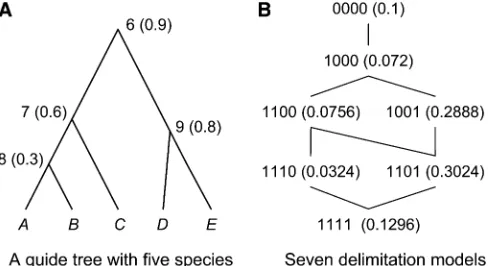
In this article, we describe two improvements to the BPP program. Thefirst is aflexible prior on species-delimitation models, by which the user assigns a prior probability that each interior node in the guide tree is a true speciation event (Figure 1). In particular, by assigning prior probability 1.0 to a speciation event one forces the two descendent popula-tions to be always recognized as distinct species. This is useful for cases in which some species delimitations are un-ambiguous as it reduces the size of the model state space and can potentially improve mixing of the MCMC. The sec-ond is a modification to our earlier rjMCMC algorithms. We modify our rjMCMC proposal to better deal with the strong constraint that the gene trees place on the species tree when the algorithm splits one species into two. Note that under the multi-species coalescent model (Rannala and Yang 2003) two sequences can coalesce only if they are in the same species (population). Thus, when we split one species into two, the youngest coalescent time (node age of a gene tree) between the two populations across all loci forms a maximum bound to the new species divergence time. With many loci, this bound can be too tight (too close to zero). In this article, we remove the upper bound and instead mod-ify the gene trees using a rubber-band algorithm (Rannala and Yang 2003) to remove incompatibilities between the gene trees and the new species divergence time in the split move. We apply the new algorithm to two empirical data sets and conduct a small-scale simulation study to demon-strate that the modifications lead to moderately improved performance.
Theory
As far as possible, we use the same notation as in Yang and Rannala (2010). Let L = {Li} be the set of species-delimitation models specified by the guide tree (Figure 1), whereLidenotes species-delimitation modeli. The data,D, consists of the alignments of nucleotide sequences at multiple loci. The population genetic parameters of species-delimitation model iinclude species divergence times t and population sizesu, collectively denotedvi= {t,u} (Yang and Rannala 2010). For simplicity, we drop the subscripts and takeLand vto indicate any particular delimitation or set of population parameters, respectively, unless the subscripts are needed in the context. The Bayesian rjMCMC algorithm generates the posterior distribution
fðL;v;GjDÞ}fðLÞfðvjLÞfðGjL;vÞfðDjGÞ;
wheref(L) andf(v|L) are the prior probabilities for delim-itationLand population genetic parametersv, respectively,
f(D|G) is the likelihood of the sequence data given the gene trees (see,e.g., Felsenstein 1981), andf(G|L,v) is the prior density of gene trees specified under the neutral multispe-cies coalescent model (Rannala and Yang 2003). Note that there is a gene tree G with associated branch lengths (co-alescence times) at every locus. Given the speciation model and population genetic parameters, the gene trees at each locus have independent distributions (we assume that the loci are unlinked). We focus on the marginal probabilities of species-delimitation models, f(L|D), integrating over the gene trees and the coalescent times (G). To reduce the num-ber of species-delimitation models to be evaluated we re-quire the user to specify a guide tree of populations and evaluate only those species-delimitation models that can be generated by collapsing nodes on the guide tree (Figure 1) (Yang and Rannala 2010).
Flexible prior for species-delimitation models
probability 0.9·(120.6) ·(120.8) = 0.072. Thefirst term in the product is the probability that node 6 is present and the last two terms are the probabilities that nodes 7 and 9, respectively, are absent. In this case, node 8 is absent with probability 1.0 because its ancestor node 7 is absent. Note that the model probabilities sum to 1 as required (Figure 1). The new prior allows the user to specify arbitrary prior probabilities for the species-delimitation models. One use of this prior is to assign a prior of one to nodes that represent well-established species divergences, so that certain species-delimitation models, such as that of one species, are disallowed by the prior. This strategy may be useful for improving mixing, as both BPP 2.1c and BPP 2.2 are sometimes noted to become trapped in the one species model, in analyses of both real and simulated data sets, even if the model has negligibly small posterior probabil-ities. At the start of a run the BPP program prints out a list of all species-delimitation models allowed by the guide tree and their prior probabilities. The user should examine this output to ensure that the prior is reasonable. The program also implements two other prior models on species delimitations: thefirst assigns equal probabilities for different labeled histories (Yang and Rannala 2010) and the second assigns equal probabilities for different rooted trees.
Rubber-band algorithm with proportional scaling
The poor mixing of the rjMCMC algorithms of Yang and Rannala (2010) appears to be caused by the strong con-straint posed by the gene trees when a new species diver-gence time (ti) is proposed in the split move. When we split a node on the guide tree, the gene trees (topology and branch lengths) are not changed. Our model assumes that two sequences can coalesce only if they belong to the same species. Consider that node i, which has descendent nodes
jandk, is a candidate for splitting into two species. In the current model (where jandk are a single species) the co-alescence time between sequences fromjandkcan be arbi-trarily small. In the proposed model (where j and k are separate species) the coalescent time between the two sequences must be older than the species divergence time ti. Thus the minimum coalescent time between sequences from j and k over all loci constitutes an upper bound tU
when we propose a new t*
i. As a result, the proposed t*i can be unrealistically small, leading to the rejection of the proposal (Figure 2A).
Here we modify the algorithm to allow larger values to be proposed for the new divergence time ti during the split move, modifying at the same time the coalescent times (node ages) in the gene trees to avoid conflicts between the gene trees and the proposed species tree. We adapt our previously developed rubber-band algorithm Rannala and Yang (2003) to achieve this. If the node to be split is not the root of the (guide) species tree, we simply use the age of the ancestral node as the upper bound. To determine a reasonable upper bound fortwhen the root node is split,
we scan the sequence alignments at loci and calculate the average sequence distance between the two sides of the root. Let this be di for locus i. The di’s have expectation
d¼tþu=2 and variance v = (u/2)2 + (u/2). Note that
the coalescent times have an exponential distribution among loci with mean (u/2) and variance (u/2)2and, conditional
on the coalescent time, the number of mutations has a Pois-son distribution. Thus from the meandand variancevofdi over loci, we get
~
u¼pffiffiffiffiffiffiffiffiffiffiffiffiffiffi4vþ121;
~
t¼d2~u=2: (1)
Those estimates do not appear to be stable and provide only rough estimates ofuandt. We set the upper bound for the newttotU¼~tþui, where~tis given in Equation 1 and does not change during the MCMC whileuiis the current value for the node to be split and changes during the MCMC algorithm. Figure 2 (A) In the old algorithm (Yang and Rannala 2010), the gene trees are not changed during the split and join moves. To split one species into two, the upper boundtUfor the new species divergence time,t*, is
given by the youngest node age between sequences from the two species across all loci. Here two gene trees are shown, with the youngest node between populations A and B marked by circles. (B) In the new algorithm,
tUis determined without scanning the gene trees. Aftert*is generated,
node ages in each gene tree are modified to avoid conflicts. Affected nodes (c1,c2, marked by squares) have descendents in both populations A and B and must be older thant*. Their ages are pushed up to be older than t*using the rubber-band algorithm. Within-move clades (clades
aandb, nodes marked by circles) have descendents in population A only or in population B only. Their ages are not restricted and are modified proportionally relative to the age of their immediate ancestor that is an affected node: the ages ofa1anda2are modified relative to the age of
Given the upper bound,tU, we construct a beta-distribution
to generate the newt* for the split move. The density is
fðt*;tU;p;qÞ ¼ 1
Bðp;qÞ
t* tU
p21 12t*
tU q21
1
tU; 0,t*,tU: (2)
This is equivalent to assuming that the transformed variable
x=t*/tUhas the familiar two-parameter beta-distribution:
xbeta(p,q) with 0,x,1. The distribution has mean tUp/(p+q) and variancet2Upq=½ðpþqÞ
2
ðpþqþ1Þ, so that larger values of p andq mean that the proposal density is more concentrated. In practice, p = 2 and q = 8 provide good performance. This beta-proposal is now used for the non-root nodes as well; the power distribution of Yang and Rannala (2010) is no longer used.
Aftert* is generated, we scan the gene trees and modify them to avoid conflicts. At each locus, we define anaffected nodeas a node in the gene tree that resides in current spe-ciesi(the candidate node for split) and that has descendents in both populationsjandk. Letmbe the number of affected nodes. The age of each affected node,t, must be older than t* and so we modify it as
tU2t* tU2t ¼
tU2t* tU20;
so that
t*¼t*þ
12t* tU
t and t¼tUðt*2t*Þ
tU2t* :
This is the rubber-band algorithm of Rannala and Yang (2003) (i.e., their Equation A.7). The gene trees are then scanned to identify so-called within-move clades. A within-move clade is a descendent of an affected node whose nodes all reside either in population j (or its descendents) or in population k (or its descendents). The ages of nodes in a within-move clade do not have to be older thant* so their ages are transformed proportionally upward by the affected node. The ages of all nodes of a within-move clade are mul-tiplied by a proportionality factorc.1 that is the ratio of the new age to the old age for the affected node (see Figure 2B). This proportional scaling algorithm incurs a proposal ratio of
cw for each within-move clade, where w is the number of nodes in the within-move clade (Yang 2006, p. 170). This is done for all within-move clades. Suppose that collectively all nodes in the within-move clades incur a proposal ratio ofC.
For the reverse join move, the affected nodes are identified in the same way. The age of each affected node with current agetis modified as
t*¼tUðt2t*Þ tU2t* :
Again the within-move clades are identified and the ages of nodes in each within-move clade are multiplied by c, the
ratio of the new age, t*, to the old age, t, for the affected node. Note that c , 1. Again, letC be the proposal ratio incurred by all nodes in the within-move clades. Instead of Equations 4 and 5 in Yang and Rannala (2010), the accep-tance ratios are
Rsplit¼
x y
pðL*Þ
pðLÞ tUðeu*jÞðeu*kÞ
tU2t*
tU m
C;
and
Rjoin¼
x y
pðL*Þ pðLÞ
1 tUðeujÞðeukÞ
tU tU2t
m C;
wherep(L) denotes the product of the prior and likelihood for delimitationL.
Computational Efficiency of New Algorithm
We conducted a small simulation study and analyzed two empirical data sets to assess the performance of the new algorithm in comparison with that of Yang and Rannala (2010), using BPP version 2.2 and BPP version 2.1c, respec-tively. Our focus here is on computational efficiency. Al-though the new prior (with probabilities assigned to nodes of the guide tree) may be used to change the posterior model probabilities, by disallowing the one-species model, for example, we envisage that this will be done only when there is overwhelming evidence in the sequence data (and possibly from other sources) against the disallowed models. In short, we expect the old and new algorithms to support the same biological conclusion if both have converged. It is thus the computational effort required to calculate the same posterior model probabilities to the same precision that we are measuring. We used two measures of computational efficiency. The first is the average model-jump probability or acceptance rate of between-model moves (Pjump). Unlike
within-model MCMC for which intermediate acceptance rates are optimal, for between-model moves a higher accep-tance rate in general means higher efficiency (see Discus-sion). The second measure is the variance (or standard deviation) of the estimated posterior model probability, with smaller variance indicating higher efficiency.
Simulation study
We simulated sequence data on the tree of five species illustrated in Figure 3. We used parameter values ofu= 0.02 for all populations and tAB = 0.01, tABC = 0.02, tABCD=
0.03, andtABCDE= 0.04. We analyzed the data in three ways:
probability 0.5. This corresponds to a case in which there is strong support for four species (C, D, E, and AB) but some uncertainty about whether A and B are good species. The data sets generated in our simulation are of this nature. Two independent sequence data sets were simulated on the tree of Figure 3 using the program MCcoal (distributed in the BPP package), with 3 sequences sampled from each of the 5 species (15 sequences in total for each locus). We simulated 15 loci for each data set, each composed of 1000 bp, under the JC69 model. Each data set was analyzed using 100 independent MCMC runs with random starting species-delimitation models and parameter values for each set of conditions (300 runs in total). The runs were carried out with 20,000 burn-in iterations and 100,000 sample itera-tions (sampling every 2 iteraitera-tions) to estimate the posterior model probabilities and to compare the efficiency of esti-mates obtained using the three different algorithms. Because we use an identical number of iterations, the relative efficiency is informative about the statistical performance of each algo-rithm given afixed computational effort. We also compared the run times of the different algorithms (see below) as the new moves will incur some computing cost, potentially in-creasing the run time for a given number of iterations. The acceptance rate for between-model moves was recorded. Ac-ceptance rates varied little among runs analyzing the same data set and using the same algorithm.
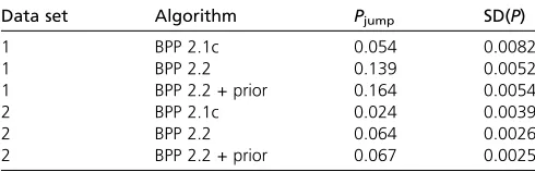
The results (Table 1) show a large increase in the accep-tance rate of between-model moves in the new algorithms. The rubber-band algorithm alone produces a nearly three-fold increase in the acceptance rate over the algorithm of Yang and Rannala (2010) for data set 1 (an increase from 5 to 14%) and the use of the prior constraint further improves acceptance by2%. Similarly, for data set 2 there is a near threefold increase (from 2.4 to 6.4%) due to the rubber-band algorithm and a further increase of about half a percent due to the prior constraint. The absolute improvement in this case is smaller because the posterior probability for data set 2 is larger than for data set 1 (0.95vs.0.82). The max-imum acceptance rate possible for data set 2 is 0.05·2 = 0.10 while that for data set 1 is 0.18 ·2 = 0.36 (see Dis-cussion). In both cases, the achieved acceptance rate is about half the theoretical maximum. The efficiency of the MCMC estimates of the posterior model probabilities is also increased due to the improved mixing. Relative to the algorithm of Yang and Rannala (2010), we see a35% reduction in the stan-dard deviation of the posterior probability among replicate runs in the new rubber-band algorithm with prior constraint in both data sets. This translates to a threefold increase in efficiency since relative efficiency is measured by the ratio of the variances of the estimates.
An additional set of 100 independent MCMC runs were performed on data set 1 to compare the performance of BPP 2.2 either using only the 6 sequences from species A and B or instead using all 15 sequences from species A, B, C, D, and E and a prior that places probability 1.0 on all nodes except the node-splitting populations A and B, which has
prior probability 0.5. This allows one to compare both the efficiency (and acceptance probabilities) for these two strategies of delimiting two species and also the resulting posterior probabilities. By including the additional sequen-ces for species C, D, and E one potentially includes additional information about shared parameters that
in-fluence the posterior probability that A and B are separate species. The results (Table 2) suggest that strategy 2 (using
fixed outgroup species) is superior to strategy 1 (using sequences from A and B only). First, the probability that A and B are distinct species, Pr(AB), is larger (0.82vs. 0.28) under strategy 2, indicating that this approach has more power. Second, Pjump is more than four times larger under
strategy 2 despite the fact that the larger Pr(AB) makes it harder to jump between models. Third, the standard devia-tion is nearly three times smaller under strategy 2, so that the Markov chain is about nine times more efficient. Figure 3 Species tree offive species used for simulation study.
Table 1 Summary of results for 100 independent MCMC analyses of two simulated data sets using each of three different algorithms
Data set Algorithm Pjump SD(P)
1 BPP 2.1c 0.054 0.0082
1 BPP 2.2 0.139 0.0052
1 BPP 2.2 + prior 0.164 0.0054
2 BPP 2.1c 0.024 0.0039
2 BPP 2.2 0.064 0.0026
2 BPP 2.2 + prior 0.067 0.0025
We compared the run times of the old algorithm (BPP 2.1) and the new one (BPP 2.2), with and without an informative prior, in analyses of the two simulated data sets. The same number of iterations (120,000) and the same computer are used. For data set 1 the run times (in minutes and seconds) for BPP 2.1, BPP 2.2 with a prior constraint, and BPP 2.2 without a prior constraint were 19:10, 19:45, and 19:46, respectively, and for data set 2 they were 19:32, 19:49, and 19:29. Thus, the improvement in efficiency of the new algorithm appears to add no extra computational cost.
Analysis of real data
We analyze two empirical data sets to evaluate the computational efficiency of the different rjMCMC algorithms discussed in this article. In all data sets we tested, the new algorithm (BBP2.2) was more efficient (as judged by improved acceptance rate and reduced standard error of the posterior model probability). The performance differ-ence, however, depends on the particular data set and parameter settings of the analysis.
The lizard data set:Thefirst data set we analyze is a nuclear exon (RAG-1) from coast horned lizards, published by Leaché et al. (2009). Leaché et al. (2009) sequenced two nuclear exons (RAG-1: 132 sequences, 529 bp, and BDNF: 136 sequences, 1100 bp), as well as two fragments of the mitochondrial genome (1.6 kb in total), to investigate the speciation history of the coast horned lizard species complex (Phrynosoma). They quantified a diversity of operational species criteria, including divergence in mitochondrial DNA and nuclear loci, ecological niches, and cranial horn shapes. The phylogenetic analysis of mtDNA recoveredfive phylogeographic groups arranged latitudinally along Cali-fornia and Baja CaliCali-fornia. The phylogeny among thosefive populations (phylogeographic groups) is used as the guide tree in our analysis (Figure 4). If we used both nuclear loci, the species-delimitation model 1111, which hasfive species, had posterior probability 100%. Here we use one locus, the RAG-1 exon, to evaluate the rjMCMC algorithms.
We used a burn-in period of 104 iterations, so that the
chain is very likely to have reached stationarity. After the burn-in, the chain was run for either 2 · 105 or 8 · 105
iterations, using rjMCMC algorithm 0 (withe = 2) in Yang and Rannala (2010, Equation 3). We analyzed the data in
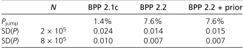
three ways, as in the analysis of the simulated data: (1) using BPP 2.1c, which implements the algorithms of Yang and Rannala (2010); (2) using BPP 2.2, which implements the rubber-band algorithm with proportional scaling; and (3) using BPP 2.2, with the new prior constraint in addition to the rubber-band algorithm with proportional scaling. The prior constraint is specified as (((NCA, SCA):0.5, (NBC, CBC):0.5):0.8, SBC):1.0; so that the five species-delimita-tion models 1000, 1100, 1101, 1110, and 1111 are assigned prior probabilities 1/5 each, while model 0000 is assigned prior probability 0. The priors on parameters are t G(2, 1000) for the root on the guide tree anduG(2, 100) for all u’s. Very long chains using all three methods gave the posterior probabilities for delimitation models 1111 and 1110 as 0.58 and 0.42, respectively. In other words, the only uncertainty in the Bayesian analysis concerns the species status of the Northern Baja California (NBC) and Central Baja California (CBC) populations. We ran each algorithm 100 times, using different starting species tree models and parameter values. The results are summarized in Table 3. Compared with BPP2.1c, the rubber-band algorithm and proportional scaling implemented in BPP2.2 increased the Table 2 Summary of results for 100 independent MCMC analyses
of simulated data set 1 using two strategies
Data and Analysis Pjump SD(P) Pr(AB)
BPP 2.2 (AB only) 0.036 0.0137 0.28
BPP 2.2 (ABCDE) + constraint 0.164 0.0054 0.82
Strategy 1 analyzes only the 6 sequences from species A and B. Strategy 2 analyzes all 15 sequences from the 5 species with the prior constraint that all populations except A and B are distinct species (that is, with probability 1.0 assigned on all nodes except the node ancestral to A and B in Figure 3).Pjumpis the average acceptance rate. SD(P) is the standard deviation (across runs) of the posterior prob-ability of the true model (1111). Pr(AB) is the estimated posterior probprob-ability that populations A and B are good species.
Figure 4 The guide tree forfive populations of coast horned lizard (
Phry-nosoma): NCA (Northern California), SCA (Southern California), NBC (Northern Baja California), CBC (Central Baja California), and SBC (South-ern Baja California). Those populations were identified by Leachéet al.
model-jump probability from 1.4 to 7.6%, a more thanfi ve-fold improvement. The maximum limit to Pjump is 2(1 2
0.58) = 0.84, achievable if all parameters (including u’s, t’s, and the gene trees) are proposed from their posterior during the split and join moves. Compared with this limit, thePjumpvalues achieved in both BPP 2.1c and 2.2 are very
low. Consistent with the improved model-jump probability, the different runs of the same algorithm are more consistent, with smaller SDs for P(1111), the posterior for the
best-fitting model, in BPP2.2 than in BPP2.1c. The variance ratio is 2–3 and suggests that the new algorithm is two to three times more efficient in estimating the posterior model probability.
The results for the two chain lengths (N) (Table 3) are consistent with our expectation that increasing the number of iterations by fourfold halves the standard deviation. The prior constraint had virtually no effect on eitherPjumpor SD
(P) in this comparison (Table 3). However, the prior is useful for preventing the chain from getting stuck at model 0000 (one species).
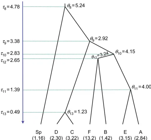
The cavefish data set: The second data set we analyze consists of 22 individuals of a cavefish (Typhlichthys subterra-neus) sequenced atfive nuclear gene loci (with one allele for each individual at each locus), published by Niemiller et al.
(2012). T. subterraneus is a teleostfish widely distributed in Eastern North America. Species delimitation based on mor-phology in subterranean animals such as cavefish is difficult as morphological differentiation is often obscured by conver-gent evolution. Genetic data thus constitute a valuable source of information for species delimitation in such organisms. Niemiller et al. (2012) sequenced multiple loci to delimit species in T. subterraneus. They used the method of O’Meara
(2010) to assign individuals to populations/species and then *BEAST (Heled and Drummond 2010) to infer the species tree. The authors conclude that the genetic data do not support the picture of a single, widely distributed species ofT. subterraneus. Instead, there exist several cryptic species with only slight morphological divergence.
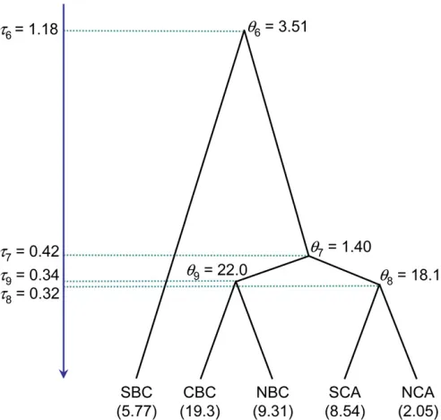
The authors nevertheless found that both the species assignment and species tree inference were sensitive to the number of individuals and the number of genes sampled, indicating that alternative strategies for generating the species guide tree should be explored. Here we use the 20-individual 6-gene data set of Niemiller et al. (2012) to evaluate the rjMCMC algorithms implemented in the differ-ent versions of BPP. We exclude the mitochondrialnd2locus and use the five nuclear loci only (s7, rag1,myh6,plagl2, andtbr1). The guide tree derived by Niemilleret al.(2012, Figure 4) is used (Figure 5). We use the same settings (pri-ors, number of iterations, etc.) as in the analysis of lizard data set, except that rjMCMC Algorithm 1 (witha= 2 and
m= 1) of Yang and Rannala (2010, Equation 6) is used. Posterior means of t’s and u’s when the guide tree is treated as a fixed species tree are shown in Figure 5. Rela-tive to the estimates for the lizard data set (Figure 4), theu’s
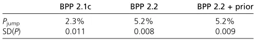
are comparable but thet’s are larger, indicating that thefish populations are genetically more divergent than the lizards. Computational efficiencies of the different rjMCMC algo-rithms are summarized in Table 4. Compared with BPP2.1c, the rubber-band algorithm and proportional scaling imple-mented in BPP2.2 increased the model-jump probability from 2.3 to 5.2%. The SDs for P(111111), the posterior probability for the-delimitation model 111111, is smaller in BPP2.2 than in BPP2.1c. The results suggest that the modifications we have introduced here generally cause bet-ter gene trees to be proposed, with improved acceptance rates, whatever the algorithm for proposing model parame-ters in the rjMCMC move (Yang and Rannala 2010).
The informative prior (Figure 5) disallows four delimita-tion models (000000, 100000, 110000, and 110001) and assigns the prior probability 0.125 to the eight remaining delimitation models. This does not lead to improvements in the acceptance rate or the precision of the posterior model probability. However, the prior constraint is effective in pre-venting the chain from getting stuck at the one-species model.
Discussion
The rjMCMC algorithm is very flexible in terms of possible proposals. However, it often suffers from poor mixing when applied to real data. This is particularly true when the data are highly informative and the posteriors of the parameters within each model are highly concentrated. Proposed between-model jumps tend to be rejected, so that the chain becomes trapped in one model, even if that model has low posterior probability. It is more difficult to construct efficient proposals for rjMCMC than for conventional MCMC. In conventional MCMC, the distance between the current value and the proposed value of a parameter can be used to adjust the acceptance rate and to construct an optimal algorithm, but in rjMCMC we lack such a measure of distance. For example, in conventional MCMC using a sliding-window proposal for a continuous target distribution, a small win-dow size will lead to small moves with Pjump1, whereas
a large window size will lead to large moves and a small
Pjump. Therefore, if the window size is adjusted to obtain
a near-optimal Pjump, the conventional MCMC algorithm
can work well regardless of whether the posterior is concen-trated or diffuse. In rjMCMC, there is no obvious parallel to such a scale adjustment because there is no guide as to what Table 3 The average model-jump probabilityPjumpand the standard
deviation for the posterior probability for the delimitation model 1111, SD(P), in 100 replicate runs of three rjMCMC algorithms
N BPP 2.1c BPP 2.2 BPP 2.2 + prior
Pjump 1.4% 7.6% 7.6%
SD(P) 2·105 0.024 0.014 0.015
SD(P) 8·105 0.010 0.007 0.007
is a“local move”when the chain is jumping between mod-els. As Green and Hastie (2009) pointed out, “For across-model proposals the lack of a concept of closeness means that frequently it is the problem of low acceptance probabil-ities that makes efficient proposals hard to design; it is usual for across-model moves to display much lower acceptance probabilities than within-model moves.”
We note here several important differences between conventional MCMC and cross-model rjMCMC. First, for within-model MCMC, there is an optimal acceptance pro-portion (say 30–40% for 1-D moves). For cross-model rjMCMC, the higher Pjump is, the more efficient the chain
tends to be (Peskun 1973). Second, Pjump is maximized by
proposing parameters for the new model from its posterior. Third, for conventional MCMC,Pjumpcan be made arbitrarily
close to 1 by decreasing the step size. With rjMCMC, the posterior model probabilities place an upper bound onPjump;
it cannot exceed twice one minus the posterior probability of the best-fitting model. ThusPjump0 does not necessarily
mean poor mixing. If the best model has posterior probabil-ity 99.9%, the chain must stay in the model 99.9% of the time and it therefore cannot accept .0.1% of the pro-posals to move away from it.
With conventional MCMC, taking a sufficiently small step virtually guarantees acceptance (although the resulting chain may mix slowly). One might think that the same would apply to rjMCMC and that to move from a simpler
model (with fewer parameters) to a more complex one (with more parameters), proposing parameter values for the more complex model that closely correspond to the current parameters of the simpler model would guarantee accep-tance. This is not the case for rjMCMC, yet it appears to be a widespread misconception concerning rjMCMC proposals. For example, Brooks et al. (2003) describe a “weak non-identifiability centering” proposal based on this idea that they claim will lead to high probabilities of between-model jumps (in fact, they argue that between-model acceptance rates of 1 can be achieved using this proposal). Clearly this is incorrect because the acceptance rate is always limited by the posterior probability of the best model. If one model dominates in the posterior, the acceptance rate of be-tween-model moves can never be high. The prior, if it is diffuse, also works against the parameter-rich model. Even though the likelihood stays essentially the same, the pro-posal is very likely to be rejected.
The mixing problems discussed here are due to the change of dimensions and/or change of probability spaces in between-model moves, that is, the change from the probability space of one model to the probability space of another model. Here we are not using Green’s formalism in which all models share one general space (Green and Hastie 2009), but consider each model having its own probability space. Mixing problems can arise in moves between models of the same dimension, but a change of dimension introdu-ces additional difficulty. While Green (2003) suggested that mixing problems may have more to do with high dimension-ality than with change of dimension, our experience is somewhat different. The within-model MCMC algo-rithms implemented in BPP have been successfully used to analyze as many as 50,000 loci (Burgess and Yang 2008), which involves extremely high dimensions in the gene trees and node ages, but the program may begin to have mixing problems with small numbers of loci when using rjMCMC for species delimitation.
Recognizing the difficulty of achieving generic improve-ments to rjMCMC algorithms due to some of the problems outlined above, in this article we focused on improving the rjMCMC mixing of the species-delimitation program by making algorithmic modifications that are specific to our particular model. First, we have modified our algorithm to jointly propose divergence times and multilocus gene trees to reduce the strong constraint that species divergence time
vs. gene-tree conflicts impose during the split move, which leads to reduced acceptance rates. This constraint becomes increasingly severe with the addition of more loci and/or sequences in the old algorithm. The rubber-band algorithm we implemented helps to reduce the effect of this constraint and results in a several-fold improvement in the accep-tance rates of between-model jumps. The between-model jump acceptance rates are still often much less than the theoretical maximum, however, suggesting that other improvements remain to be found. A second modification changed the prior on the guide tree to allow certain species Figure 5 The guide tree for seven populations of cavefish (Typhlichthys),
delimitations to be given larger prior probability (even a probability of 1.0). This allows biologists to incorporate other sources of information in the analysis and helps in reducing the dimension of the inference problem without reducing sequence information (as would occur if one re-moved the species with fixed delimitations, for example). Analyses of the simulated data indicated that including ad-ditional species withfixed delimitations could increase pos-terior probabilities for target group of species and also helps to improve the mixing of the rjMCMC.
We note that in analyses of both real and simulated data sets the posterior probability of the bestfitting model tends to increase quickly with the addition of more loci, with the posterior probability for one model reaching 100% when between 10 and 20 loci are used (Zhanget al.2011). While genome-scale data sets are becoming increasingly common, there appears to be no need to use hundreds of loci for the purpose of species delimitation. Instead it may be more im-portant to examine variable patterns of species divergences across the genome, as speciation-related adaptation is likely to leave signals in isolated regions of the genome (Dasmahapatra
et al.2012).
BPP2.2, which implements the new algorithms developed in this article, is distributed at its website athttp://abacus. gene.ucl.ac.uk/software/. The program is written in ANSI C and can be compiled on various platforms. Both the coast horned lizard and the cavefish data sets are included in the package as example data sets.
Acknowledgments
We thank Adam Leaché for providing the coast horned liz-ard data set and Matthew Niemiller for the cavefish data set. We thank two anonymous referees and the associate editor for comments. We are grateful to the participants of the National Institute for Mathematical and Biological Synthesis (NIMBioS) working group on species delimitation for many useful suggestions for modifications of Bayesian phyloge-netics and phylogeography. Part of this research was com-pleted while the authors were guests of the Institute of Zoology, Chinese Academy of Sciences, Beijing, supported by the Center for Computational and Evolutionary Biology. B.R. completed part of this work while on sabbatical at the Laboratory of Alpine Ecology, Grenoble, France. B.R. received support from National Institutes of Health grant
R01-HG01988. Z.Y. is supported by a Biotechnological and Biological Sciences Research Council (UK) grant and a Royal Society/Wolfson Merit Award.
Literature Cited
Brooks, S. P., P. Giudici, and G. O. Roberts, 2003 Efficient con-struction of reversible jump Markov chain Monte Carlo proposal distributions. J. R. Stat. Soc. B 65: 3–39.
Burgess, R., and Z. Yang, 2008 Estimation of hominoid ancestral population sizes under Bayesian coalescent models incorporat-ing mutation rate variation and sequencincorporat-ing errors. Mol. Biol. Evol. 25: 1979–1994.
Camargo, A., M. Morando, L. J. Avila, and J. W. Sites, 2012 Species delimitation with ABC and other coalescent-based methods: a test of accuracy with simulations and an em-pirical example with lizards of theLiolaemus darwiniicomplex (Squamata: Liolaemidae). Evolution 66: 2834–2849.
Dasmahapatra, K. K., J. R. Walters, A. D. Briscoe, and J. W. Davey, 2012 Butterfly genome reveals promiscuous exchange of mim-icry adaptations among species. Nature 487: 94–98.
Ence, D. D., and B. C. Carstens, 2011 SpedeSTEM: a rapid and accurate method for species delimitation. Mol Ecol Res 11: 473– 480.
Felsenstein, J., 1981 Evolutionary trees from DNA sequences: a maximum-likelihood approach. J. Mol. Evol. 17: 368–376. Green, P. J., 2003 Trans-dimensional Markov chain Monte Carlo,
pp 179–196 inHighly Structured Stochastic Systems, edited by P. J. Green, N. L. Hjort, and S. Richardson. Oxford University Press, Oxford, UK.
Green, P. J., and D. I. Hastie, 2009 Reversible jump MCMC. Available at: http://www.stats.bris.ac.uk/peter/papers/rjmcmc_20090613. pdf. Accessed: February 16, 2012.
Heled, J., and A. J. Drummond, 2010 Bayesian inference of spe-cies trees from multilocus data. Mol. Biol. Evol. 27: 570–580. Knowles, L. L., and B. C. Carstens, 2007 Delimiting species
with-out monophyletic gene trees. Syst. Biol. 56: 887–895.
Leaché, A. D., M. S. Koo, C. L. Spencer, T. J. Papenfuss, R. N. Fisher et al., 2009 Quantifying ecological, morphological, and ge-netic variation to delimit species in the coast horned lizard spe-cies complex (Phrynosoma). Proc. Natl. Acad. Sci. USA 106: 12418–12423.
Niemiller, M. L., T. J. Near, and B. M. Fitzpatrick, 2012 Delimiting species using multilocus data: diagnosing cryptic diversity in the southern cavefish, Typhlichthys subterraneus (Teleostei: Am-blyopsidae). Evolution 66: 846–866.
O’Meara, B. C., 2010 New heuristic methods for joint species de-limitation and species tree inference. Syst. Biol. 59: 59–73. Peskun, P. H., 1973 Optimum Monte-Carlo sampling using
Mar-kov chains. Biometrika 60: 607–612.
Rannala, B., and Z. Yang, 2003 Bayes estimation of species di-vergence times and ancestral population sizes using DNA se-quences from multiple loci. Genetics 164: 1645–1656. Yang, Z., 2006 Computational Molecular Evolution. Oxford
Uni-versity Press, Oxford, UK.
Yang, Z., and B. Rannala, 2010 Bayesian species delimitation us-ing multilocus sequence data. Proc. Natl. Acad. Sci. USA 107: 9264–9269.
Zhang, C., D.-X. Zhang, T. Zhu, and Z. Yang, 2011 Evaluation of a Bayesian coalescent method of species delimitation. Syst. Biol. 60: 747–761.
Communicating editor: M. A. Beaumont Table 4 The average model-jump probability Pjump and the
standard deviation for the posterior probability for the delimitation model 111111, SD(P), in 100 replicate runs of three rjMCMC algorithms
BPP 2.1c BPP 2.2 BPP 2.2 + prior
Pjump 2.3% 5.2% 5.2%
SD(P) 0.011 0.008 0.009