Optimization of a Hybrid Energy Storage System for Electric Vehicles Using Machine Learning Methods

(1)

University of Windsor University of Windsor

Scholarship at UWindsor

Electronic Theses and Dissertations Theses, Dissertations, and Major Papers

2016

Optimization of a Hybrid Energy Storage System for Electric

Vehicles Using Machine Learning Methods

Eric Lesiuta

University of Windsor

Follow this and additional works at: https://scholar.uwindsor.ca/etd

Recommended Citation Recommended Citation

Lesiuta, Eric, "Optimization of a Hybrid Energy Storage System for Electric Vehicles Using Machine Learning Methods" (2016). Electronic Theses and Dissertations. 5837.

https://scholar.uwindsor.ca/etd/5837

This online database contains the full-text of PhD dissertations and Masters’ theses of University of Windsor students from 1954 forward. These documents are made available for personal study and research purposes only, in accordance with the Canadian Copyright Act and the Creative Commons license—CC BY-NC-ND (Attribution, Non-Commercial, No Derivative Works). Under this license, works must always be attributed to the copyright holder (original author), cannot be used for any commercial purposes, and may not be altered. Any other use would require the permission of the copyright holder. Students may inquire about withdrawing their dissertation and/or thesis from this database. For additional inquiries, please contact the repository administrator via email

(2)

Optimization of a Hybrid Energy Storage System for Electric Vehicles Using Machine Learning Methods

By

Eric J. Lesiuta

A Thesis

Submitted to the Faculty of Graduate Studies

through the Department of Electrical and Computer Engineering

in Partial Fulfillment of the Requirements for

the Degree of Master of Applied Science

at the University of Windsor

Windsor, Ontario, Canada

2016

(3)

Optimization of a Hybrid Energy Storage System for Electric Vehicles Using Machine Learning Methods

by

Eric J. Lesiuta

APPROVED BY:

______________________________________________

B. Minaker

Department of Mechanical, Automotive and Materials Engineering

______________________________________________

K. Tepe

Department of Electrical and Computer Engineering

______________________________________________

N. Kar, Advisor

Department of Electrical and Computer Engineering

(4)

iii

Declaration of Originality

I hereby certify that I am the sole author of this thesis and that no part of

this thesis has been published or submitted for publication.

I certify that, to the best of my knowledge, my thesis does not infringe upon

anyone’s copyright nor violate any proprietary rights and that any ideas,

techniques, quotations, or any other material from the work of other people

included in my thesis, published or otherwise, are fully acknowledged in

accordance with the standard referencing practices. Furthermore, to the

extent that I have included copyrighted material that surpasses the bounds

of fair dealing within the meaning of the Canada Copyright Act, I certify that

I have obtained a written permission from the copyright owner(s) to include

such material(s) in my thesis and have included copies of such copyright

clearances to my appendix.

I declare that this is a true copy of my thesis, including any final revisions,

as approved by my thesis committee and the Graduate Studies office, and

that this thesis has not been submitted for a higher degree to any other

(5)

iv

Abstract

In electric vehicles, batteries are unable to entirely store the large amount

of power from regenerative braking which is generated over a short time

period. Batteries also have a lower efficiency when required to supply

peaking power. Alternatively supercapacitors can handle peaking power at

the expense of lower energy storage capacities. This is why hybrid energy

storage systems using a battery and a supercapacitor are being

researched. There exist multiple configurations and control strategies for

these systems and recently some are beginning to take drive cycle data

into consideration.

The objective of this research is to design an intelligent algorithm for

controlling the balancing of energy between a supercapacitor and a battery.

By using machine learning methods, it’s able to learn from offline data

where the optimal balancing can be calculated. The algorithm can then

operate online, predicting how to balance the system which should improve

(6)

v

Dedication

To my parents, Steve and Sylvia.

(7)

vi

Acknowledgements

First I would like to thank Dr. Narayan Kar for providing me with the

resources and support conducive to an exceptional learning environment.

He permitted me the freedom to find my own path allowing me to further

develop my skills as a researcher and an Engineer. I was very fortunate to

have him as a supervisor.

I would also like to thank Dr. Bruce Minaker for providing me with the

research opportunity to study regenerative braking and his assistance. His

great personality made it a pleasure working with him.

Lastly I would like to thank all my colleagues in CHARGE Labs; they were

always willing to share their knowledge and helped make the last two years

(8)

vii

List of Tables

(12)

xi

List of Figures

Figure 1.1: Flowchart of a Simple Rule Based Balancing Algorithm ... 3

Figure 3.1: Passive Parallel Hybrid Energy Storage System ... 14

Figure 3.2: Partially Decoupled Supercapacitor/Battery Configuration ... 15

Figure 3.3: Partially Decoupled Battery/Supercapacitor Configuration ... 16

Figure 3.4: Fully Decoupled Cascaded Battery/Capacitor Configuration ... 17

Figure 3.5: Fully Decoupled Cascaded Capacitor/Battery Configuration ... 17

Figure 3.6: Fully Decoupled Multiple Converter Configuration ... 19

Figure 4.1: Free Body Diagram of Vehicle ... 21

Figure 4.2: Overview of Power Transfers ... 25

Figure 5.1: A Single Node in a Neural Network ... 28

Figure 5.2: Node Connections in a Simple Neural Network ... 29

Figure 5.3: Adjusted Speed Data Sample 1 ... 32

Figure 5.4: Adjusted Speed Data Sample 2 ... 32

Figure 5.5: Power Trickle Coefficient Sample 1 ... 34

Figure 5.6: Power Trickle Coefficient Sample 2 ... 34

Figure 5.7: Neural Network Score for a Learning Rate of 0.001 ... 35

Figure 5.8: Neural Network Score for a Learning Rate of 0.005 ... 36

Figure 5.9: Histogram of Parameter Biases for Layer 0 ... 36

(13)

xii

Figure 5.11: Histogram of Parameter Biases for Layer 1 ... 37

Figure 5.12: Histogram of Parameter Weights for Layer 1 ... 38

Figure 5.13: Histogram of Gradient Weights ... 39

Figure 5.14: Flowchart of the Machine Learning Policy for a Hybrid Energy Storage System ... 41

Figure 5.15: Rule Based Policy Step 0 ... 43

Figure 5.16: Rule Based Policy Step 1 ... 43

Figure 5.17: Rule Based Policy Step n ... 43

Figure 5.18: Offline Policy Step 0 ... 44

Figure 5.19: Offline Policy Step 1 ... 44

Figure 5.20: Offline Policy Step n ... 44

Figure 5.21: Machine Learning Policy Step 0 ... 45

Figure 5.22: Machine Learning Policy Step 1 ... 45

Figure 5.23: Machine Learning Policy Step n ... 45

Figure 6.1: Speed vs Time for Trip 9 ... 47

Figure 6.2: Acceleration vs Time for Trip 9 ... 48

Figure 6.3: Power Demand vs Time for Trip 9 ... 49

Figure 6.4: Battery Energy Usage over Time ... 50

Figure 6.5: Energy Stored in the Capacitor over Time ... 50

Figure 6.6: Battery to Motor Power Transfer vs Time ... 51

Figure 6.7: Capacitor to Motor Power Transfer vs Time ... 52

Figure 6.8: Battery to Capacitor Power Transfer vs Time ... 53

(14)

xiii

Figure 6.10: Capacitor Delta Power vs Time ... 55

Figure 6.11: Offline Policy - Battery to Motor Power Transfer vs Time ... 56

Figure 6.12: Offline Policy - Capacitor to Motor Power Transfer vs Time .. 57

Figure 6.13: Offline Policy - Battery to Capacitor Power Transfer vs Time 57 Figure 6.14: Offline Policy - Total Battery Power Output vs Time ... 58

Figure 6.15: Offline Policy - Capacitor Delta Power vs Time ... 58

Figure 6.16: Battery to Capacitor Power vs Time for a Re-trained Machine Learning Policy ... 59

Figure 6.17: Rule Based Policy - Battery to Motor Power Transfer vs Time ... 60

Figure 6.18: Rule Based Policy - Capacitor to Motor Power Transfer vs Time ... 61

Figure 6.19: Rule Based Policy - Battery to Capacitor Power Transfer vs Time ... 61

Figure 6.20: Rule Based Policy - Total Battery Power Output vs Time ... 62

Figure 6.21: Rule Based Policy - Capacitor Delta Power vs Time ... 62

Figure 6.22: Trip 9 - Battery Energy Usage vs Time ... 64

(15)

xiv

(16)

xv

List of Abbreviations/Symbols

Label Description

𝑎 Acceleration of vehicle

𝐴𝑓 Frontal area

𝐵𝐶 Power transfer from battery to capacitor

𝐵𝑀 Power transfer from battery to motor

𝐶 Rated capacity of battery

𝑐_𝑑 Coefficient of drag

𝐶𝑀 Power transfer from capacitor to motor

𝐶_𝑝 Capacity at one-ampere discharge rate

𝐹𝑎𝑖𝑟 Force of air resistance

𝐹𝐵 Total braking force on vehicle

𝐹_𝑏 Total desired braking force

𝐹_𝑓 Front axle braking force

𝐹_𝑔 Force due to gravity

𝐹𝐻𝑓 Front axle hydraulic braking force

(17)

xvi

𝐹_𝑚 Braking force of the motor

𝐹_{𝑚 𝑚𝑎𝑥} Maximum braking force of the motor

𝐹𝑚𝑜𝑡𝑜𝑟 Force provided by motor on vehicle

𝐹𝑛𝑒𝑡 Net force on vehicle

𝐹_𝑟𝑟 Force of rolling resistance

𝑔 Acceleration due to gravity

𝐻 Rated discharge time

𝐼 Actual discharge rate of battery

𝑘 Peukert constant

𝑘_𝑏 Braking force coefficient

𝐾_𝑐 An arbitrary constant

𝑘_𝑧 Braking strength coefficient

𝑚 Vehicle mass

𝑃 Power

𝑃_𝑖 Point object

𝑆 Brake pedal travel

𝑇𝑖 Power transfer object

𝑣 Vehicle velocity

𝑉_{𝑏𝑎𝑡𝑡} Voltage across the battery

𝑉_𝑐𝑎𝑝 Voltage across the supercapacitor

𝑉_𝐷𝐶 Voltage across the DC bus

(18)

xvii

𝛽 Original braking distribution coefficient

𝜂 Efficiency

𝜃 Angle above the horizontal

𝜇𝑟 Coefficient of rolling resistance

(19)

1

Chapter 1

1 Introduction

1.1 Background

In order for electric vehicles to be as efficient as possible, they need to take full

advantage of all the energy that is available to them. Regenerative braking is an

excellent piece of technology that assists with this by capturing otherwise wasted

energy and storing it in the battery. However, there is still more potential to

improve this system since batteries are unable to store all the regenerative power

in such a short amount of time. In addition, batteries have a lower efficiency

when required to handle peaking power demands, and therefore waste energy.

Supercapacitors have the opposite characteristics of batteries, in that they can

handle peaking power demands and store large amounts of power over a short

time at the expense of a smaller capacity [1]. This makes them an ideal

candidate to combine with batteries in a hybrid energy storage system. Hybrid

energy storage systems are actively being researched due to their potential for

reducing power loss compared to systems that use only a battery [2]–[6].

In order for a hybrid energy storage system to realize its full potential, it requires

an effective control scheme for balancing energy between both energy sources.

(20)

2

increasing computational power onboard vehicles and the huge advancements

with machine learning, there is great potential for improving the control schemes

even further.

1.2 Literature Review

Since electric vehicle require a high storage capacity such as that of a battery,

and the ability to efficiently handle peaking power such as that of a capacitor,

hybrid energy storage systems are being researched to meet both

requirements[6], [7]. These systems offer a lot of freedom in how they are

controlled, which can significantly affect their efficiency. Rule based control

methods are based on human knowledge of the system to create a set of rules

that dictate exactly what will happen under different conditions. This approach is

limited in the fact that every possibility has to be thought of ahead of time along

with how the system should behave should something unexpected happen. An

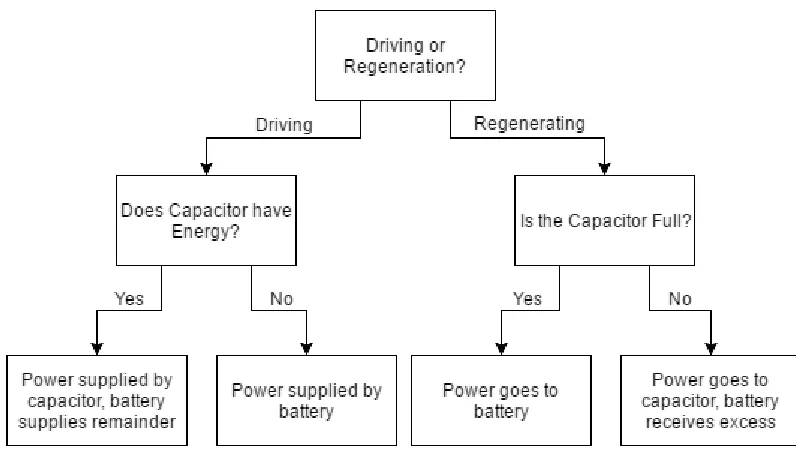
example of a very simple rule based is shown below in Fig. 1.1. This flowchart

presents the decisions a simple rule based algorithm would take in balancing

(21)

3

Figure 1.1: Flowchart of a Simple Rule Based Balancing Algorithm

Although the above figure may work, it is very general and the results are not

optimal. This is what is classified as a thermostat type of rule based strategy.

This is because all the decisions are either yes or no, thus turning the options on

or off. An alternative to this is the fuzzy rule based method where parameters can

take on a range of values, which is better suited for real time data [6], [10], [11].

Rule based control strategies can be improved significantly by adding many

different cases [12]. The cases can have varying degrees of specificity, where

one can have a large number of different cases to find optimal outputs for each

one. However this can be a daunting task and produce a codebase that is difficult

to maintain. These cases could include any type of driving or sensor data,

(22)

4

The approach to optimizing hybrid energy storage systems can either be

analytical or numerical, where the goal is to minimize a cost function. The cost

function could be something along the lines of how much power was used over

the duration of the trip, and could include other factors such as wear and tear on

certain components, such as the brakes or battery cells [15]. There are two main

categories of optimization methods. The first is offline optimization, which has full

knowledge (past, present and future) of all power demands through the entire

drive cycle at every point in the simulation. The other category is online

optimization, which is given the data in a piecewise fashion so it only has

knowledge of past and present power demands [16]–[18].

In the following chapters of this thesis an online control strategy utilizing neural

networks to learn from a given optimal offline control algorithm will be discussed.

Both strategies will then be tested and compared against a new set of data to

determine how competitive the online algorithm is.

1.3 Research Outline

The goal of this research is to develop and test an intelligent balancing algorithm

for a hybrid energy storage system that can be used to run in real time. The first

step is to examine how these systems currently work and where they have the

(23)

5

deciding on which technique would be best suited for the task. In the case of

using machine learning techniques, not only are there many methods to choose

from, there is nearly an infinite number of ways they could be trained. How a

machine learning algorithm learns has an immense impact on its results. Once a

suitable method is chosen, it must be properly implemented and trained to

become useful for improving the balancing of a hybrid energy storage system

such that it saves power.

In order to validate the algorithm, a detailed simulation is required. The simulator

would need to be able to work with real world Global Positioning System (GPS)

data and accurately model the power requirements of the vehicle at each given

point in the GPS trip data. It would then need to be capable of running an

arbitrary balancing algorithm for a hybrid energy storage system and testing it

against a model of a supercapacitor and a battery to determine the energy

losses. Running multiple different types of balancing algorithms will allow for a

comparison between their performance and for drawing a conclusion of the

results.

1.4 Thesis Structure

This thesis consists of seven chapters. In Chapter 1, the research topic and

motivation, along with an outline are introduced. Chapter 2 provides a literature

(24)

6

hybrid energy storage systems is provided. Different hybrid energy storage

system configurations are discussed along with their various benefits and

shortcomings. In Chapter 4, the vehicle model used to simulate different hybrid

energy storage systems and validate this research is discussed. Model equations

and a step-by-step description of how the simulation works are given. Chapter 5

provides an in depth look at neural networks and how they are used to design an

intelligent control scheme for a hybrid energy storage system. A flow chart of the

balancing algorithm is given. In Chapter 6 the results of the simulation are

provided and discussed. Finally Chapter 7 discusses the implications of this

(25)

7

Chapter 2

2 Regenerative Braking

2.1 Introduction to Regenerative Braking

Regenerative braking is a method of braking where the vehicle’s kinetic energy is

converted back into a form where it can be stored and used again. This is

contrary to traditional braking which relies on using friction to slow the vehicle

and the energy is wasted by being dispelled as heat [19]. These systems

increase the complexity of already existing braking system designs and their

implementation must not interfere with the vehicle’s ability to stop quickly and

reliably [20].

Regenerative braking is unable to capture all the vehicle’s energy and slow the

vehicle at the same rate as traditional brakes, so they are typically used side by

side, with a fraction of the force going to each [1], [21]. Since some of the braking

torque is now provided by the motor, this also increases the lifespan of the

traditional brakes, allowing them to last about twice as long by reducing the wear

on the brake pads [22]. One of the limiting factors in regenerative braking’s ability

to capture energy is the rate at which it can be stored in a battery. This is why

some systems have been proposed with dual energy sources. Typically in these

(26)

8

a battery has a high energy density, allowing it to store larger amounts of energy,

the rate at which it can receive the energy, or power, is lower than the rate

regenerative braking can generate it. A supercapacitor on the other hand can

receive and transmit power at much high rates, so it can be used as a sort of

buffer to take in the excess power generated by the regenerative braking above

which the battery can handle [23]. It can then be used to assist in powering the

motor. Using a supercapacitor in conjunction with a battery provides other

benefits as well such as prolonging the life of the battery since the capacitor can

now be trickle charged by the battery to help handle peaks in acceleration [3], [6].

2.2 Safety Considerations of Regenerative Braking

Since the braking performance is a crucial factor to the overall safety of the

vehicle, the system must be capable of sufficiently reducing the vehicle’s speed

while maintaining directional control via the steering wheel [24]. To meet this

requirement, the braking torque applied must both be great enough and be

distributed properly amongst the wheels. Usually the required braking torque is

greater than the torque an electric motor can produce on its own so another

method of mechanical braking must be included along with regenerative so as to

(27)

9

One method of including traditional braking with regenerative braking is a parallel

hybrid braking system. This is where all the conventional mechanical

components are included, so the system will still contain brake calipers and discs

along with ABS. Only the regenerative braking force is electronically controlled,

however the mechanical braking force is still controlled by the driver through the

brake pedal or ABS when the wheels are about to lock if it’s included. The largest

challenge of this design is being able to recover as much energy as possible [1].

In addition to traditional brakes where there is a mechanical link between the

brake actuators and the pedal, different methods of electronic braking systems

are being researched. In these systems there are multiple methods of applying a

mechanical braking torque to the wheel to dissipate the energy as heat, but the

braking actuator is electrically linked to the pedal and controlled by software

instead of a mechanical link. This is done with the aim to improve regenerative

braking by improving the braking control over individual wheels. These systems

are still in the early stages of development [24]–[26]. In these systems, it is

possible to control the braking force through each wheel individually. This is

(28)

10

2.3 Balancing Load between Regenerative and

Traditional Brakes

The electric motor needs to be controlled in order to provide the desired amount

of braking force requested by the driver while maximising regeneration.

Regenerative braking is typically only effective when used on the driven axle

which for the majority vehicles is the front axle [1]. There exist many control

schemes for balancing the braking force between regeneration and traditional

brakes [27], [28].

A typical weighting algorithm for regenerative braking would use only traditional

brakes at low speeds below a certain threshold such as 15 km/hr or when ABS is

engaged. The reason for this is at low speeds or when the wheels are close to

locking, it is difficult to produce torque from the electric motor due to the low

electromotive force being generated. At speeds above the given threshold and

when the braking force requested is low, all the braking force can be provided by

the regenerative brakes [1].

An example of a simple weighting algorithm is described by the following

equations given by [27]. Where 𝐹_𝐵 and 𝐹_𝑏 are the total braking force on the

vehicle and the desired braking force respectively. 𝐹𝐻𝑓 and𝐹𝐻𝑟 are the front and

rear axle hydraulic braking forces. 𝐹_𝑚and 𝐹_{𝑚 𝑚𝑎𝑥} are the actual and maximum

braking force of the motor. 𝐹_𝑓 is the total front axle braking force. 𝛽 is the original

(29)

11

and 𝑘_𝑏 are the braking strength, braking strength coefficient, and braking force

coefficients respectively. Finally, S is the brake pedal travel.

𝐹𝐵 = 𝑚𝑧𝑔 (2.1)

𝑧 = 𝑘𝑧𝑆 (2.2)

𝐹_𝐵 = 𝑘_𝑏𝑆 (2.3)

𝑘_𝑏 = 𝑚𝑔𝑘_𝑧 (2.4)

Equations 2.5-2.7 are for 𝑧 ≤ 0.15.

𝐹_𝑚 = { 𝐹𝑏 (𝐹𝑏 ≤ 𝐹𝑀 𝑀𝑎𝑥) 𝐹_{𝑀 𝑀𝑎𝑥} (𝐹_𝑏 > 𝐹_{𝑀 𝑀𝑎𝑥})

(2.5)

𝐹_𝐻𝑓 = { 0 (𝐹𝑏≤ 𝐹𝑀 𝑀𝑎𝑥) (𝐹𝑏− 𝐹𝑀 𝑀𝑎𝑥)β (𝐹𝑏> 𝐹𝑀 𝑀𝑎𝑥)

(2.6)

𝐹𝐻𝑟 = {

0 (𝐹𝑏 ≤ 𝐹𝑀 𝑀𝑎𝑥)

(𝐹𝑏− 𝐹𝑀 𝑀𝑎𝑥)(1 − β) (𝐹𝑏 > 𝐹𝑀 𝑀𝑎𝑥)

(2.7)

Equations 2.8-2.11 are for 0.15 < 𝑧 ≤ 0.3.

𝐹_𝑓 = 0.8 𝐹_𝑏 (2.8)

𝐹_𝑚 = { 𝐹𝑓 (𝐹𝑓 ≤ 𝐹𝑀 𝑀𝑎𝑥) 𝐹_{𝑀 𝑀𝑎𝑥} (𝐹_𝑓 > 𝐹_{𝑀 𝑀𝑎𝑥})

(2.9)

𝐹_𝐻𝑓 = { 0 (𝐹𝑓 ≤ 𝐹𝑀 𝑀𝑎𝑥) (𝐹𝑓− 𝐹𝑀 𝑀𝑎𝑥)β (𝐹𝑓> 𝐹𝑀 𝑀𝑎𝑥)

(2.10)

𝐹𝐻𝑟 = {

0.2𝐹𝑏 (𝐹𝑓 ≤ 𝐹𝑀 𝑀𝑎𝑥)

(𝐹𝑓− 𝐹𝑀 𝑀𝑎𝑥)(1 − β) + 0.2Fb (𝐹𝑓 > 𝐹𝑀 𝑀𝑎𝑥)

(2.11)

Equations 2.12-2.15 are for 0.3 < 𝑧 ≤ 0.6.

𝐹_𝑓 = 𝐹_𝑏𝛽 (2.12)

𝐹_𝑚 = { 𝐹𝑓 (𝐹𝑓 ≤ 𝐹𝑀 𝑀𝑎𝑥) 𝐹_{𝑀 𝑀𝑎𝑥} (𝐹_𝑓 > 𝐹_{𝑀 𝑀𝑎𝑥})

(30)

12

𝐹𝐻𝑓 = {

0 (𝐹𝑓≤ 𝐹𝑀 𝑀𝑎𝑥)

𝐹_𝑓− 𝐹_{𝑀 𝑀𝑎𝑥} (𝐹_𝑓 > 𝐹_{𝑀 𝑀𝑎𝑥})

(2.14)

𝐹_𝐻𝑟 = (1 − 𝛽)𝐹_𝑏 (2.15)

Equations 2.16-2.18 are for 𝑧 > 0.6.

𝐹_𝑚 = 0 (2.16)

𝐹_𝐻𝑓 = 𝐹_𝑏𝛽 (2.17)

𝐹_𝐻𝑟 = (1 − 𝛽)𝐹_𝑏 (2.18)

This is a relatively simple weighting algorithm which incorporates regenerative

braking with traditional braking on both the front and rear axles. In these

balancing equations, there does not appear to be a smooth transition between

regenerative braking and mechanical braking when the driver requests different

braking strengths (𝑧) across the four different ranges. There are many other

weighting algorithms; all of which seek to maximise energy regeneration without

sacrificing the safety and control of the vehicle’s braking performance [1], [27],

(31)

13

Chapter 3

3 Energy Management Systems

3.1 Introduction to Energy Management Systems

Energy management systems in electric vehicles are responsible for controlling

the flow of power between the vehicle’s energy storage, motor, and various

electronics. They do so through the use of power electronics such as DC-DC

converters and inverters. As power electronics improve, adding additional

components to electrical vehicles, such as those required for a hybrid energy

storage system, becomes more practical. Currently the battery is one of the most

expensive components of an electric vehicle, so it is imperative to have an

effective energy management system that allows it to be used as efficiently as

possible [6], [7], [30], [31].

This chapter will begin with a review of some of the different topographies for

hybrid energy storage systems. The next part of this chapter will introduce

(32)

14

3.2 Basic Topographies

3.2.1 Passive Parallel Configuration

Figure 3.1: Passive Parallel Hybrid Energy Storage System

The basic passive parallel topography shown in Fig. 3.1 is the simplest

configuration [4] . The supercapacitor is essentially just a low pass filter for the

battery. In this configuration the voltage of each component is simply represented

by Equation 3.1.

𝑉𝐵𝑎𝑡𝑡 = 𝑉𝐶𝑎𝑝 = 𝑉𝐷𝐶 (3.1)

The voltage changes experienced by the DC bus are very slow and miniscule as

the bus is directly clamped to the terminals of the battery unit. This is desirable

for the input voltage of the DC-AC converter. Since there are no active

components between the battery and the supercapacitor, not much can be done

(33)

15

3.2.2 Partially Decoupled Supercapacitor/Battery Configuration

Figure 3.2: Partially Decoupled Supercapacitor/Battery Configuration

The supercapacitor/battery configuration shown in Fig. 3.2 uses a bidirectional

DC-DC converter to interface to the supercapacitor. This allows the voltage of

supercapacitor to be used over a wide range, which is beneficial, while the

battery voltage has to remain constant [3], [6]. However, since the bidirectional

DC-DC converter has to be rated in accordance with the supercapacitor’s power

rating, it has to be rated higher since the supercapacitor takes on quick and large

power demand variations. This leads to a larger size and cost of the DC-DC

converter compared to the next configuration [4]. Also, since the battery unit is

connected directly to the DC bus, it is not protected from high current

(34)

16

3.2.3 Partially Decoupled Battery/Supercapacitor Configuration

Figure 3.3: Partially Decoupled Battery/Supercapacitor Configuration

Decoupling the battery from the DC bus (DC Link) shown in Fig. 3.3 protects it

from the highly fluctuating currents and allows control of the power transfer to

and from the battery [5]. The supercapacitor handles these highly fluctuating

currents which increases the efficiency of the system. The drawback however is

the DC bus may now be exposed to large voltage fluctuations instead which

would considerably decrease the efficiency of converter. This can be mitigated

effectively with a proper control strategy for the DC-DC converter, which allows

(35)

17

3.2.4 Fully Decoupled Cascaded Configuration

Figure 3.4: Fully Decoupled Cascaded Battery/Capacitor Configuration

Figure 3.5: Fully Decoupled Cascaded Capacitor/Battery Configuration

Fully decoupled configurations use two converters to decouple the battery

and the supercapacitor from the DC bus. Two different combinations of the

cascaded configuration are shown in Fig. 3.4 and Fig. 3.5.

In the configuration on the top (Fig. 3.4), the battery unit is connected behind

the supercapacitor at lower voltage terminals and the supercapacitor is

connected to DC-DC converter behind the inverter and is at an intermediate

voltage level. The benefits to this topology include it being easier to balance

battery cells at lower voltages than that at higher voltages [3]. Another benefit

(36)

18

be rated at approximately the same power rating as the battery unit, reducing

the cost. A drawback to this configuration is there are more losses at the

DC-DC converter connecting the supercapacitor to the DC-DC bus (DC-DC link) since the

voltage of the supercapacitor will fluctuate [3], [32].

Another option is to swap the positions of the battery unit and supercapacitor

as shown in Fig. 3.5. Some of the trade-offs include attaining a more stable

voltage at the higher rated DC-DC converter connected to the DC bus at the

cost of increasing the difficulty of balancing the battery unit. This is because

this DC-DC converter is connected at the intermediate voltage level therefore

the battery must also be kept at a higher voltage [6].

3.2.5 Fully Decoupled Multiple Converter Configuration

Another fully decoupled topography that provides an alternative to the cascaded

connection is the multiple converter configuration shown in Fig. 3.6. This

configuration places the supercapacitor and battery units with their own DC-DC

converters in parallel [3], [6]. Both DC-DC converters will be connected at the

same voltage level but the voltages of both the supercapacitor and battery can

be maintained independently. This increases stability of the system and allows

(37)

19

(38)

20

Chapter 4

4 Vehicle Dynamics and Simulation

4.1 Introduction to the Vehicle Model

The vehicle model provides a means for calculating the power requirements of

the energy storage system at each time step. Since the input is given as a list of

GPS coordinates (longitude, latitude, and elevation) with respect to time, the

vehicle's speed and acceleration can be calculated at each point. From there,

approximate forces on the vehicle can be used to calculate the torque

requirement from the motor giving an estimate of the power demand [1], [33].

Once the power demand is calculated at every point, the vehicle model can

simulate different energy management system policies, calculating the power

transfers between each component and how they should be balanced. This is

then simulated with the battery model to predict efficiency losses. The end result

is a calculation of the total energy required for each trip, and a comparison of

each hybrid energy storage system management policy against the baseline,

which does not use a capacitor. Although it is calculating an overall energy

savings, this number is more useful in comparing different energy management

strategies and how much better they are than others in relative terms rather than

(39)

21

4.2 External Physical Model of the Vehicle

The vehicle model is used to calculate approximately how much force the motor

is required to provide, and using a simple efficiency map, the amount of power

required as well. This allows for calculation of the approximate power

requirements at each time step in the GPS data.

Figure 4.1: Free Body Diagram of Vehicle

In Fig. 4.1 above, a free body diagram of the vehicle is shown [1], [22], [33]–[35].

The forces to the left are acting against the vehicle, with the exception of gravity

which can be for (negative) or against (positive). The force of air resistance is

shown in Equation 4.1.

𝐹_𝑎𝑖𝑟 = 1

2𝜌𝐴𝑓𝑐𝑑𝑣|𝑣|

(4.1)

where 𝜌 is air density. The density is dependent on elevation and changes during

the trip. Area is the frontal area of the vehicle. The coefficient of drag for the

vehicle is given by 𝑐_𝑑 and finally 𝑣 is velocity [1], [34].

(40)

22

𝐹_𝑟𝑟= 𝜇_𝑟𝑚𝑔 (4.2)

where 𝜇_𝑟 is the coefficient of rolling resistance, 𝑚 is the total mass of vehicle and

occupants, and 𝑔 is the acceleration due to gravity. The final equation on the left

is for weight where

𝐹_𝑔 = 𝑚𝑔𝑠𝑖𝑛(𝜃) (4.3)

where a positive 𝜃 indicates an angle above the horizontal and therefore a

positive force acting against the vehicle when going uphill.

On the right of Fig 4.1, there is the force of the motor driving the vehicle forward

which can be expressed by Equation 4.4.

𝐹_{𝑚𝑜𝑡𝑜𝑟} =𝑃𝜂 𝑣

(4.4)

where power is the amount required by the motor in watts. Efficiency is that of

the motor and assumed to be constant. When the power is negative it is

assumed to be regenerative. The magnitude of the efficiency constant used in

Equation 4.4 is decreased if the power is regenerative. This is to take into

account greater motor losses and traditional brakes applying a portion of the

braking torque. In the equation, speed is that of the vehicle. In order to solve for

power, the force required by the motor must first be calculated by finding the net

force on the vehicle [33].

(41)

23

𝐹_𝑛𝑒𝑡 = 𝑚𝑎 = 𝐹_{𝑚𝑜𝑡𝑜𝑟} − 𝐹_𝑎𝑖𝑟− 𝐹_𝑟𝑟− 𝐹_𝑔 (4.5)

where 𝑎 is the acceleration of the vehicle. Since speed, acceleration and air

density can all be calculated from the longitude, latitude, elevation and time

stamp provided by each data point in the GPS data, and all other variables are

given as constants, an estimation of the power required at each point can be

calculated [33], [36]. Although the model is relatively simple, it provides a good

enough simulation to test different energy management strategies and draw

comparisons between them.

4.3 Model of Vehicle’s Electrical Components

The model assumes a constant discharge for all the vehicle’s electronics except

for the motor power, which is calculated using model just discussed. The

supercapacitor is assumed to have a constant efficiency over its limited capacity.

The model of the battery utilizes Peukert's law [22], [33], [37]. This is given by

Equation 4.6.

𝐶𝑝 = 𝐼𝑘𝑡 (4.6)

where 𝐶𝑝 is the capacity at a one-ampere discharge rate in amp-hours, 𝐼 is the

actual discharge rate in amps, and 𝑘 is the Peukert constant which is

dimensionless and depends on the battery. The 𝑡 is the actual time to discharge

(42)

24

𝑡 = 𝐻 (𝐶 𝐼𝐻)

𝑘 _(4.7)

where 𝐶 is the rated capacity and 𝐻 is the rated discharge time in hours.

Rearranging this equation can give you Equation 4.8.

𝐼𝑡 = 𝐶 (𝐶 𝐼𝐻)

𝑘−1 _(4.8)

The effective capacity at a discharge rate of 𝐼 is given by 𝐼𝑡. From here the

efficiency can be calculated by taking the effective capacity and dividing by the

rated capacity resulting in Equation 4.9.

𝜂 = (𝐶 𝐼𝐻) 𝑘−1 _(4.9) (𝐶 𝐻) 𝑘−1

= 𝐾_𝑐 (4.10)

𝜂 = 𝐾_𝑐 × 1 𝐼𝑘−1

(4.11)

Equation 4.9 can be further simplified by separating the constant 𝐾_𝑐 as shown in

(43)

25

4.4 Complete Model Overview

The purpose of the described model is to allow simulation of different transfer

schemes between the components shown in Fig. 4.2.

Figure 4.2: Overview of Power Transfers

Power is able to transfer in either direction between these three components; the

direction of the arrow indicates a positive power flow.

Now that all the components of the model have been discussed, the simulation is

executed as following [33], [38]–[40]:

1. Begin Simulation.

2. Load GPS data from directory and parse files.

3. For each point of GPS data, calculate speed, acceleration and run through

the vehicle model calculations for power demand, saving all this data as

an array of point objects.

4. Create a battery and capacitor object with the initial conditions to keep

(44)

26

5. Instantiate the class for the energy management policy to be tested.

6. Call the energy management policy to calculate the power flows. The input

is the next point object in the array and the current state of the battery and

capacitor. The output is the power flows BC, BM, and CM shown in Fig.

4.2.

7. Test to make sure neither the capacitor or battery is overdrawn, and that

power supplied is equal to power demand; any issue will return an error.

8. Using the power flows given from the policy, and the model of the battery

and supercapacitor, update their current state.

9. If there are still more points in the array of point objects, go back to step 6.

10. Save results and end program.

There is also an alternative method of running the simulation for calculating

optimal values using an offline optimization algorithm (one that cannot run in real

time) [41]. In this version all points in the array of point objects will be available to

(45)

27

Chapter 5

5 Machine Learning

5.1 Neural Network Principles

Neural networks are a type of machine learning algorithm modeled after neurons

in the human brain. Like a real neuron, which has multiple connections

(synapses), nodes are objects in a neural network that have multiple inputs and

outputs. By connecting many of these neurons into layers forming a network,

many different types of behaviour can be modeled. The inputs and outputs can

either be a series of binary values, useful for classification or continuous

numbers when using regression.

Also like a human brain, these algorithms need to learn from training, which can

either be supervised or unsupervised. Supervised learning is when the training

data requires associated labels, typical of a classification problem such as facial

recognition. Unsupervised learning is when the input data can come with an

associated cost function to minimize. Once trained, a neural network is great at

recognizing patterns in real world data whether it is in the form of images, video,

sound, text or time series data. As long as the inputs have some correlation with

the output, they can be trained to predict or model the behaviour, and continue to

(46)

28

5.2 Elements of Neural Networks

As stated, a neural network is composed of nodes, where each individual node

behaves almost like a neuron in the brain. The nodes are organized into layers.

Every node in the first layer receives every input, with each input multiplied by its

own weight unique to that node. The sum is then taken of all the inputs multiplied

by their weights in each node and passed through an activation function that

determines whether this neuron should “fire” and what its output is [44]. A

diagram of a single node with four inputs is given in Fig. 5.1 below.

Figure 5.1: A Single Node in a Neural Network

In each of the following layers, this process is repeated, where every node

receives every input from the previous layer, multiplied by a weight, summed

together and passed through an activation function. Each layer’s output becomes

the input for the next layer [42], [45]. Fig. 5.2 shows what a three layer neural

(47)

29

hidden layer, and 2 nodes in the output layer. In a neural network it is possible to

have any number of nodes in any number of layers.

Figure 5.2: Node Connections in a Simple Neural Network

One of the common activation functions used in neural networks is the hyperbolic

tan function. This is because hyperbolic tan was found to work very well with real

world data in many cases. There are also many other functions to choose from,

for this purpose hyperbolic tan was chosen for the input layer and hidden layer;

however the output layer uses the identity function which is simply f(x) = x. This is

because the output needs to be a continuous value, not a high or low which is

better suited for classification of data where the output is binary. Only one layer

of a neural network can use the identity function otherwise the network can be

simplified into one layer meaning it no longer provides the same level of

(48)

30

can be classified as a deep learning network; however, there is no universally

agreed upon threshold for this definition.

In order for the neural network to learn, it needs a method of calculating the error

and back propagating the results to adjust all the weights at every node. One

such method is the gradient descent. This method looks at the relationship of

error and weight by calculating how a slight change in weight creates a change in

error using the chain rule of calculus to go back through the networks layers. The

process of slightly adjusting a model’s weights in response to the error is simply

repeated until the error can no longer be reduced.

5.3 Neural Networks Applied to Energy Management

Systems

5.3.1 Setting up the Network

Although neural networks have a wide array of applications, they can’t simply be

plugged into any system as a black box and expected to work. Knowledge of the

system is required in order to properly set up the network and present it with data

in a way that is useful. In this algorithm, the neural network uses the driver’s

speed history as the input. It takes an array of the speeds at the current and

(49)

31

hidden layers of 50 nodes each, followed by a single output node. The hidden

layers utilize hyperbolic tan as their activation function and the output node uses

the identity function. The output of the neural network indicates how much power

should trickle from the battery to the supercapacitor. The optimization method for

the neural network’s training is the gradient descent.

5.3.2 Data Normalization

To normalize speed data such that it works well with the neural network, the

speed in metres/second was reduced by 10, and then the result was divided by

20. This produced a distribution where most of the data falls between -1 and 1,

with the centre around 0. A normal distribution is ideal, but extremely difficult to

produce consistently with this type of real world data. Fig. 5.3 and Fig 5.4 show

examples of this distribution from two different drive cycles. Even though they are

far from normal, both distributions were still able to produce good results with the

(50)

32

Figure 5.3: Adjusted Speed Data Sample 1

(51)

33

Since a neural network performs better when the output is either in binary for

classification problems, or a range from 0-1 for regression, the neural network did

not perform well when trying to predict the transfer power from the battery to the

supercapacitor directly. To work around this, a simple rule based algorithm was

first used to calculate the base values. The neural network would then predict the

coefficient to multiply with the base value. A histogram of the predicted

coefficients from two different drive cycles is shown in Figs. 5.5 and 5.6. Fig. 5.5

corresponds to the same drive cycle shown in Fig. 5.3, and Fig. 5.6 with Fig. 5.4.

Since the power supplied by the energy storage system has to equal the power

demanded, there is not much room for improvement here. The only power

transfer that is predicted by the neural network is the trickle from the battery to

the supercapacitor. This allows the supercapacitor to help handle peaks in power

demand. The reason why power does not trickle from the supercapacitor to the

battery is because this is equivalent to the supercapacitor simply providing power

(52)

34

Figure 5.5: Power Trickle Coefficient Sample 1

(53)

35

5.3.3 Training the Neural Network

After the neural network is configured, there are still some parameters that

require tuning, and it is important to verify that the network is learning correctly.

Fig. 5.7 shows the score vs iteration of the neural network as it is learning. The

score is the error in prediction and should decrease over time if everything is

configured correctly, as it is in this case. If the score is increasing that means the

learning rate is likely set too high and is unstable. If the score is flat or decreases

too slowly, the learning rate is too low. This could also indicate problems with the

optimization algorithm chosen.

Figure 5.7: Neural Network Score for a Learning Rate of 0.001

Fig 5.8 shows what a learning rate of 0.005 looks like for this algorithm, it’s not as

(54)

36

Figure 5.8: Neural Network Score for a Learning Rate of 0.005

The other parameters to check are the biases and weights of all the nodes. Over

time they should approximate a Gaussian distribution. Fig. 5.9 and Fig. 5.10

show the biases and weights for the first layer respectively. Fig. 5.11 and Fig.

5.12 show the biases and weights for the second layer respectively. Again values

that are diverging or very large indicate that the learning rate is set too high, or if

the distribution of data being classified is very imbalanced.

(55)

37

Figure 5.10: Histogram of Parameter Weights for Layer 0

(56)

38

Figure 5.12: Histogram of Parameter Weights for Layer 1

The last thing to check is the gradients of the nodes. Again these should form a

Gaussian distribution over time. Exploding gradients are problematic for the

parameters of the neural network. This would be an indicator of an error with

weight initialization, learning rate, or an issue with the normalization of the input

(57)

39

Figure 5.13: Histogram of Gradient Weights

5.3.4 Design of Algorithm

The flowchart in Fig. 5.14 shows how the algorithm operates under the

simulation. The only difference between this and a real implementation is that the

data points would be received from the vehicle instead of the model and the

output would be fed back to the vehicle. When the algorithm is in training mode, it

also receives the power transfers calculated from the offline policy along with the

point data from the simulation. It will still produce its prediction of the best power

transfer coefficient, but now this will also be compared to the one calculated from

using the offline policy and the error can be back propagated through the

(58)

40

The type of network used is a feed forward network and utilizes deep learning

(multiple non-linear layers). Feed forward neural networks themselves have no

memory, in contrast to other types of neural networks that also use previous

outputs as part of the next input. However, the algorithm in this case does have

memory and remembers the previous driving speeds, using the previous 100 as

an input the neural network. The number of previous speeds to remember was

chosen simply because a number around 100 produced the best results and

(59)

41

(60)

42

5.3.5 Comparison of Energy Management Policies

The purpose of using the neural network is to predict the results of an optimal

offline policy such that it can be used online in a real system.

The following 9 figures depict how 3 different energy management policies go

about calculating the power transfer between components in the hybrid energy

storage system. Each input Pi is a single point, containing the longitude, latitude,

elevation, timestamp and all the variables can be calculated from them using the

model, including speed, acceleration and power demand. Each output Ti is the

power transfer between the battery and capacitor, battery and motor, and

(61)

43

The first 3 (Fig. 5.15 - 5.17) of the next 9 figures (Fig. 5.15 - Fig. 5.23) depict how

a simple rule based policy is run by the simulation at points i = 0, 1, and n.

Figure 5.15: Rule Based Policy Step 0

Figure 5.16: Rule Based Policy Step 1

(62)

44

The following 3 figures (Fig. 5.18 - Fig. 5.20) depict an offline optimization policy.

Figure 5.18: Offline Policy Step 0

Figure 5.19: Offline Policy Step 1

(63)

45

The final 3 figures (Fig. 5.21 - Fig. 5.23) depict the machine learning policy using

neural networks. It works by using only the past and present values and so can

be run online.

Figure 5.21: Machine Learning Policy Step 0

Figure 5.22: Machine Learning Policy Step 1

(64)

46

Chapter 6

6 Results

This chapter will provide an in depth look and analysis of the results generated

from the simulation of the neural network energy balancing strategy.

6.1 Simulation Setup

In order to obtain these results, the neural network needs to be trained. The GPS

data was acquired from a free public source online. Sixteen trips from a single

driver were used totalling around 400 km. The sixteen trips were randomly split

into two sets of 8 trips, each set approximately 200 km. Trips 1 through 8 were

used for the training data; 9 through 16 were used for testing. To test both the

progress training makes and the overall results, the algorithm was trained by the

trips one at a time, while retaining all previous learning. After each step in

training, the simulation was run against the entire testing set. The execution time

of the machine learning policy is fairly quick, where learning from each trip

happens in a matter of minutes and testing in a matter of seconds. It is expected

that the machine learning algorithm will learn to predict how to operate from the

offline policy and after each successive training session, approach the

(65)

47

6.2 Analysis of Drive Cycle and Power Transfers

The first trip of the testing data (trip 9) consisted of 3566 data points over a

distance of approximately 36.2km for approximately 60 minutes. This trip will be

analyzed in the most detail since it provides a good sample of city driving with

traffic and a short section along the highway. The analysis will consist of the

results from the machine learning policy after it has been trained on all 8 training

trips.

Figure 6.1: Speed vs Time for Trip 9

Fig. 6.1 shows a plot of the vehicle speed vs time over the drive cycle. Unless

otherwise indicated, in all the following plots of this chapter, the raw data is

(66)

48

thicker, solid red line. A Savitzky-Golay filter was used to smooth the data.

Although the raw data contains lots of noise, due to it being recorded with a

regular consumer device, the data is still useful for relative comparisons between

the energy management policies. The raw GPS data was also plotted and

compared with alternative programs to analyze and check for any irregularities or

errors in basic calculations such as speed.

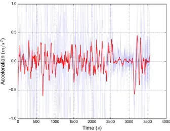
Figure 6.2: Acceleration vs Time for Trip 9

Fig. 6.2 shows an acceleration vs time plot, there is much less acceleration from

about 2500 to 3000 seconds which would be the period spent going 100 km/hr

(67)

49

Figure 6.3: Power Demand vs Time for Trip 9

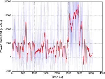
The power demanded shown in Fig. 6.3 roughly corresponds to the speed plot in

Fig. 6.1. The power demand peaks while driving on the highway at a fairly

constant speed of 100km/hr. To meet these power demands, power can come

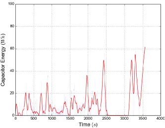
directly from either the battery, capacitor, or both. Fig. 6.4 shows a plot of the

energy stored in the battery over time as it is depleted, and Fig. 6.5 shows the

(68)

50

Figure 6.4: Battery Energy Usage over Time

(69)

51

As can be seen in Fig. 6.5, the capacitor is quite active during the stop and go

portion of the drive cycle; however, once the energy has been drained during

highway driving it no longer receives any charge until the vehicle has slowed

down. The lack of energy stored in the capacitor over this time period aligns with

the greatest power demand shown Fig. 6.3.

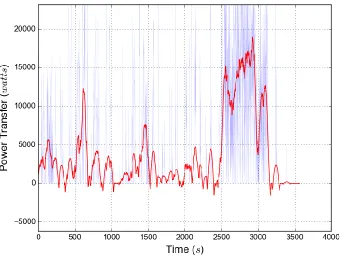
Figure 6.6: Battery to Motor Power Transfer vs Time

As shown in Fig. 6.6, the power supplied comes mainly from the battery so it

matches pretty closely with the power demand in Fig. 6.3. The smoothed data

may appear to dip below 0 at some points but that is just an artifact of smoothing

it since the raw data is completely above 0. This would indicate that the majority

of regenerative power is going to the capacitor when using the machine learning

(70)

52

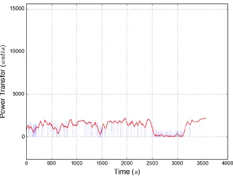
Figure 6.7: Capacitor to Motor Power Transfer vs Time

Next is the power transfer from the battery to the capacitor as can be seen in Fig.

6.8. This plays an important role in minimizing power losses and is one of the

primary differentiators between other policies. This is because it would typically

be expected that the capacitor is first in line to receive power when regenerating.

However, when the capacitor should feed the power back to the motor or receive

trickle charging from the battery is a more challenging problem. The capacitor

would not trickle charge the battery since it is more efficient to simply have the

capacitor power the vehicle and give the battery a reduced load. Ideally the

battery would transfer power to the capacitor when it can output the extra power

without adversely affecting its efficiency and it expects that it will need assistance

(71)

53

Figure 6.8: Battery to Capacitor Power Transfer vs Time

The next two figures, Fig. 6.9 and Fig. 6.10, show the overall power transfers of

both the battery and capacitor respectively. Fig. 6.9 is the addition of the battery

to motor power (Fig. 6.6) and the battery to capacitor power (Fig. 6.8). Fig. 6.10

is the difference between capacitor to motor power (Fig. 6.7) and battery to

(72)

54

Figure 6.9: Total Battery Power Output vs Time

As can be seen again by the capacitor delta power plot (Fig. 6.10), the capacitor

transfers all of its power in the first couple minutes on the highway when the

power demand peaked. It then isn’t doing much since there isn’t any braking and

(73)

55

Figure 6.10: Capacitor Delta Power vs Time

6.3 Analysis of Alternate Balancing Policies

6.3.1 Offline Optimization Policy

The following figures (Fig. 6.11 - 6.16) are now an analysis of the offline

optimization policy to see what characteristics it has. The method it used for

calculating how much power is supplied by the motor and capacitor is similar to

that of the machine learning policy and the rule based policy, where it differs

again is the battery to capacitor power transfer. The results it obtained was

(74)

56

possible battery to capacitor power trickles and selecting the one with the lowest

cost. Since it only tests from a set of levels, that is why Fig. 6.13 is already

relatively smooth with low noise. This is also one of the reasons why its results

aren’t always the best possible, as will be shown in the few cases where the

Machine Learning Policy was able to perform better.

Figure 6.11: Offline Policy - Battery to Motor Power Transfer vs Time

(75)

57

Figure 6.12: Offline Policy - Capacitor to Motor Power Transfer vs Time

(76)

58

Figure 6.14: Offline Policy - Total Battery Power Output vs Time

(77)

59

The basic trends of the offline optimization policy are similar to the machine

learning policy however when closely comparing their shapes, they’re quite

different. One significant difference between the offline policy and the machine

learning policy is in during the highway potion. The offline policy trickles power

from the battery to the capacitor which is not recommended since it is at a lower

efficiency when transferring too much power. It is curious why the machine

learning policy did not pick up this habit, since it learned from the offline policy.

To investigate this, a plot of the battery to capacitor transfer power over time is

made from the case where the neural network only trains on trip 9, and is then

tested against only trip 9.

Figure 6.16: Battery to Capacitor Power vs Time for a Re-trained Machine Learning Policy

As is shown in Fig. 6.16, the machine learning policy’s battery to capacitor power

transfer now more closely resembles the one for the offline policy, including the

(78)

60

for this is the offline algorithm may stumble upon a local maximum in the way it

checks for possible lowest cost values. This mistake in the offline optimization

policy could also be why the machine learning policy performed better in the last

few test runs as it received additional training. As long as mistakes such as these

are few, the machine learning algorithm has some tolerance, which would

theoretically improve with the more good data it is given.

6.3.2 Rule Based Policy

Fig. 6.17 - 6.21 show the power transfers for the rule based policy.

(79)

61

Figure 6.18: Rule Based Policy - Capacitor to Motor Power Transfer vs Time

(80)

62

Figure 6.20: Rule Based Policy - Total Battery Power Output vs Time

(81)

63

Again the overall trends of the rule based policy are similar to the other two

policies; however, the shape of the plotted data varies quite a bit. This would be

because the basic idea of using the capacitor to handle peaks in power is

common, but how they go about it on a finer level in closer detail is different.

When simply looking at the plots of power transfers between different

components on their own, it is difficult to immediately recognize which one would

belong to each policy or which one would perform better.

6.4 Summary

In order to compare the performance of the policies on a per trip basis, plots of

the battery energy drainage for each policy are shown in the following figures

(82)

64

Figure 6.22: Trip 9 - Battery Energy Usage vs Time

(83)

65

(84)

66

(85)

67

(86)

68

As one can see, the machine learning policy performs closely to the offline policy

from which it learned. The small discrepancies between them are likely due to

random chance since real world data can never be perfectly predicted. Since the

machine learning policy was based off the same rules as the rule based policy

but with a modifier coefficient that the neural network learns from training with the

offline policy, this demonstrates that neural network was able to make an

improvement based on the simulation results.

Policy Energy Usage Mileage Energy Savings

Baseline (no capacitor) 31.94 kWh 6.360 km/kWh 0%

Rule Based 31.73 kWh 6.404 km/kWh 0.684%

Offline Optimization 31.23 kWh 6.505 km/kWh 2.274%

Machine Learning Trip 1 31.59 kWh 6.431 km/kWh 1.118%

(87)

69

Figure 6.30: Results Summary

As shown in table 6.1 and the resulting scatter plot (Fig. 6.30) of the training data

learning over the 8 trips, the machine learning algorithm usually performed better

after each successive training session until it peaked around 2.3%. Machine

learning trip 1 through 8 indicate how many of the training trips the policy has

learned from, and is tested against trips 9 through 16 each time. With a properly

implemented and trained neural network, the overall trend expected is that the

more it is trained, the better it performs. Slight dips are typical as long as the

overall trend is an improvement. It was not expected that it would perform better

than the offline optimization policy in the last three runs. Since the neural network

used this policy to learn from, at best it should approach but not reach the same

performance. The fact that it did is likely due to random chance for this test data,

Optimization of a Hybrid Energy Storage System for Electric Vehicles Using Machine Learning Methods

Scholarship at UWindsor

Scholarship at UWindsor

Optimization of a Hybrid Energy Storage System for Electric

Optimization of a Hybrid Energy Storage System for Electric

Vehicles Using Machine Learning Methods

Vehicles Using Machine Learning Methods

Declaration of Originality

Abstract

Dedication

Acknowledgements

Table of Contents

List of Tables

List of Figures

List of Abbreviations/Symbols

Chapter 1

1 Introduction

1.1 Background

1.2 Literature Review

1.3 Research Outline

1.4 Thesis Structure

Chapter 2

2 Regenerative Braking

2.1 Introduction to Regenerative Braking

2.2 Safety Considerations of Regenerative Braking

2.3 Balancing Load between Regenerative and

Traditional Brakes

Chapter 3

3 Energy Management Systems

3.1 Introduction to Energy Management Systems

3.2 Basic Topographies

3.2.1 Passive Parallel Configuration

3.2.2 Partially Decoupled Supercapacitor/Battery Configuration

3.2.3 Partially Decoupled Battery/Supercapacitor Configuration

3.2.4 Fully Decoupled Cascaded Configuration

3.2.5 Fully Decoupled Multiple Converter Configuration

Chapter 4

4 Vehicle Dynamics and Simulation

4.1 Introduction to the Vehicle Model

4.2 External Physical Model of the Vehicle

4.3 Model of Vehicle’s Electrical Components

4.4 Complete Model Overview

Chapter 5

5 Machine Learning

5.1 Neural Network Principles

5.2 Elements of Neural Networks

5.3 Neural Networks Applied to Energy Management

Systems

5.3.1 Setting up the Network

5.3.2 Data Normalization

5.3.3 Training the Neural Network

5.3.4 Design of Algorithm

5.3.5 Comparison of Energy Management Policies

Chapter 6

6 Results

6.1 Simulation Setup

6.2 Analysis of Drive Cycle and Power Transfers

6.3 Analysis of Alternate Balancing Policies

6.3.1 Offline Optimization Policy

6.3.2 Rule Based Policy

6.4 Summary