Cultural Algorithm based on Decomposition to solve Optimization Problems

(1)

University of Windsor University of Windsor

Scholarship at UWindsor

Electronic Theses and Dissertations Theses, Dissertations, and Major Papers

9-20-2019

Cultural Algorithm based on Decomposition to solve Optimization

Problems

Ramya Ravichandran University of Windsor

Follow this and additional works at: https://scholar.uwindsor.ca/etd

Recommended Citation Recommended Citation

Ravichandran, Ramya, "Cultural Algorithm based on Decomposition to solve Optimization Problems" (2019). Electronic Theses and Dissertations. 7835.

https://scholar.uwindsor.ca/etd/7835

This online database contains the full-text of PhD dissertations and Masters’ theses of University of Windsor students from 1954 forward. These documents are made available for personal study and research purposes only, in accordance with the Canadian Copyright Act and the Creative Commons license—CC BY-NC-ND (Attribution, Non-Commercial, No Derivative Works). Under this license, works must always be attributed to the copyright holder (original author), cannot be used for any commercial purposes, and may not be altered. Any other use would require the permission of the copyright holder. Students may inquire about withdrawing their dissertation and/or thesis from this database. For additional inquiries, please contact the repository administrator via email

(2)

Cultural Algorithm based on

Decomposition to solve

Optimization Problems

By

Ramya Ravichandran

A Thesis

Submitted to the Faculty of Graduate Studies

through the School of Computer Science

in Partial Fulfillment of the Requirements for

the Degree of Master of Science

at the University of Windsor

Windsor, Ontario, Canada

2019

(3)

Cultural Algorithm based on

Decomposition to solve

Optimization Problems

By

Ramya Ravichandran

APPROVED BY:

______________________________________________ K. Tepe

Department of Electrical and Computer Engineering

______________________________________________ S. Samet

School of Computer Science

______________________________________________ Z. Kobti, Advisor

School of Computer Science

(4)

iii

DECLARATION OF CO-AUTHORSHIP

/ PREVIOUS PUBLICATION

1. Co-authorship

I hereby declare that this thesis incorporates material that is the result of

research conducted under the supervision of Dr. Ziad Kobti. In all cases, the key

ideas, primary contribution, experimental designs, data analysis, and

interpretation were performed by the author, and the contribution of the

co-author was primarily through the proofreading of the published manuscripts.

I am aware of the University of Windsor Senate Policy on Authorship, and

I certify that I have properly acknowledged the contribution of other researchers

to my thesis, and have obtained written permission from each of the co-author(s)

to include the above material(s) in my thesis.

I certify that, with the above qualification, this thesis, and the research to

which it refers, is the product of my work.

2. Previous Publication

This thesis includes one original paper that has been previously submitted

(5)

iv

Section Publication title/ Full citation Publication status

3, 4 Ramya Ravichandran and Ziad Kobti “

Solving Dynamic Multi-Objective

Optimization Problem Using Cultural

Algorithm based on Decomposition.” In 2019

International Symposium on Computing and

Artificial Intelligence (ISCAI 2019),

Vancouver, Canada.

Accepted

I certify that I have obtained a written permission from the copyright

owner(s) to include the above published material(s) in my thesis. I certify that the

above material describes work completed during my registration as a graduate

student at the University of Windsor.

3. General

I declare that, to the best of my knowledge, my thesis does not infringe

upon anyone's copyright nor violate any propriety rights and that any ideas,

techniques, quotations, or any other material from the work of other people

included in my thesis, published or otherwise, are fully acknowledged in

(6)

v

that I have included copyright material that surpasses the bounds of fair dealing

within the meaning of Canada Copyright Act, I certify that I have obtained

written permission from the copyright owner to include such material in my

thesis.

I declare that this is a true copy of my thesis, including any final revisions,

as approved by my thesis committee and the Graduate Studies Office, and that

this thesis has not been submitted for a higher degree to any other University or

(7)

vi

ABSTRACT

Decomposition is used to solve optimization problems by introducing

many simple scalar optimization subproblems and optimizing them

simultaneously. Dynamic Multi-Objective Optimization Problems (DMOP) have

several objective functions and constraints that vary over time. As a consequence

of such dynamic changes, the optimal solutions may vary over time, affecting the

performance of convergence. In this thesis, we propose a new Cultural Algorithm

(CA) based on decomposition (CA/D). The objective of the CA/D algorithm is to

decompose DMOP into a number of subproblems that can be optimized using the

information shared by neighboring problems. The proposed CA/D approach is

evaluated using a number of CEC 2015 optimization benchmark functions. When

compared to CA, Multi-population CA (MPCA), and MPCA incorporating game

strategies (MPCA-GS), the results obtained showed that CA/D outperformed

(8)

vii

DEDICATION

I would like to dedicate this thesis to my family

Father: Ravichandran Egappan

Mother: Janagi Ravichandran

(9)

viii

ACKNOWLEDGMENTS

There are many people I would like to thank for the successful completion

of my master thesis. First and foremost, I would like to express my sincere

gratitude to my supervisor, Dr. Ziad Kobti, for his continuous support of my

research study, for his patience, motivation, enthusiasm, and immense

knowledge. He helped me in accomplishing my goals and has provided valuable

guidance in improving research skills. It was a great pleasure to work and discuss

with him. I would also like to appreciate the time he dedicated for me and the

funding he provided me to complete this thesis. Without his support, this thesis

would not be complete.

I would also like to thank my committee members – Dr. Tepe and Dr. Samet – whose inputs and suggestion have given a better shape to my research. I also would like to thank the support of Mrs. Melissa, Mrs.Christine, and Mrs.

Gloria for helping with various academic issues.

I am very thankful to my parents and friends who gave me the strength,

moral support, and unconditional love, which kept me motivated to pursue my

research. Last but not least, I would like to thank God for giving this excellent

(10)

ix

LIST OF TABLES

Table 5.1: Summary of the CEC 2015 Benchmark problems [21]. . . .56

Table 5.2 Parameter values for the algorithm. . . .70

Table 5.3: M1-M5 on F1-F7 for 10D. . . 71

Table 5.4: M1-M5 on F8-F15 for 10D. . . .72

Table 5.5: M1-M5 on F1-F7 for 30D. . . .74

(14)

xiii

LIST OF FIGURES

Figure 1.1 Pseudo-code for EA [23] . . . 10

Figure 3.1: Relation between Genomes and Phenomes [46] . . . 32

Figure 3.2: Types of crossover operations [14] . . . 36

Figure 3.3: Types of Mutation [14] . . . 37

Figure 3.4: Architecture of CA [12] . . . 40

Figure 4.1: Phenotypic normative part . . . 46

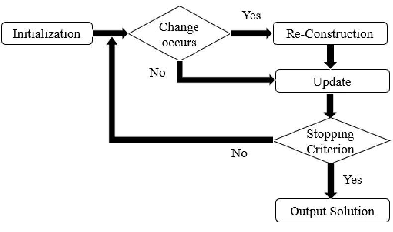
Figure 4.2: Flowchart of the Algorithm. . . 56

Figure 5.1: 3D-Map for Rotated Bent Cigar Function [29] . . . 57

Figure 5.2: 3D – Map for Rotated Discus Function [29] . . . 58

Figure 5.3: 3D –Map for Rotated and Shifted Schwefel’s Function [29] . . . .59

Figure 5.4: 3D -Map for Rotated and Shifted Katsuura Function [29]. . . 60

Figure 5.5: 3D – Map for Rotated and Shifted HappyCat Function [29]. . . 60

Figure 5.6: 3D – Map for Rotated and Shifted HGBat Function [29]. . . 61

Figure 5.7: 3D –Map for Shifted and Rotated Scaffer’s F6 Function [29]. . . 62

(15)

xiv

Figure 5.9: 3D – Map for Composite Function 2 [29] . . . .67

Figure 5.10: 3D – Map for Composite Function 3 [29] . . . 68

Figure 6.1: Convergence performance of M2, M3 and M4 for F4 (30D) . . . 83

Figure 6.2: Convergence performance of M1, M3 and M4 for F11 (30D) . . . .84

Figure 6.3: Convergence performance of M2, M3 and M5 for F6 (30D) . . . .85

(16)

xv

LIST OF ABBREVIATIONS

EA Evolutionary Algorithms

CA Cultural Algorithms

SOP Single Optimization Problem

MOP Multi-Objective Problem

DMOP Dynamic Multi-Objective Optimization Problem

DOP Dynamic Optimization Problem

GA Genetic Algorithms

DE Differential Evolution

POS Pareto Optimal Solutions

POF Pareto Optimal Front

CR Convergence Ratio

NSGA-II Non-Dominated Sorting Genetic Algorithm – II

FPS Feed-Forward Population Strategy

PPS Prediction-based Population Strategy

MOEA/D-DP Differential Prediction incorporated by Multi-Objective

Optimization Evolutionary Algorithm based on Decomposition

KF Kalman Filter

SGEA Steady-State and Generational Evolutionary Algorithm

MRP-MOEA Multiple Reference Point – MOEA

CAEP Cultural Algorithm with Evolutionary Programming

(17)

xvi

MPCA Multi Population Cultural Algorithm

HMPCA

TM

RP

Hetrogeneous Multi Population Cultural Algorithm

Tchebycheff Method

(18)

1

Chapter 1 Introduction

1.1 Background

Optimization problems involve finding one or more effective and efficient

solution(s) from a pool of feasible solutions. In other words, it involves finding

the best solution by maximizing the desired factors and minimizing undesired

factors [30]. Evolutionary Algorithms (EA) have been widely used by researchers

to solve complex optimization problems. EA contains a search space which

focuses on the optimization of the problem and searches for the best possible

solution [14]. The search space in EA comprises exploration and exploitation

operators. Exploration means finding new points in different areas of the search

spaces, which has not been investigated before. On the other hand, exploitation is

the process of improving and combining the traits of the currently known

solutions [31]. The solutions generated can be near-optimal or optimal. While

EAs are successfully applied to various types of optimization problems, they

(19)

2

generations. Diversity can be maintained between the population by using

Cultural Algorithms (CA). CA is a class of EA which is most likely used to solve

multi-objective problems (MOP). Introducing decomposition of the MOP in CA

can address the issue of immature convergence (finding solutions as close as

possible to Pareto optimal front) as decomposing the problem into many

subproblems, enhances the search for best solutions which shows good potential

for better results.

Decomposition is a traditional and primary method used to solve

multi-objective problems. As the name suggests, it decomposes a multi-multi-objective

optimization into many simple scalar optimization subproblems, and also

optimizes these problems simultaneously [1]. Using Decomposition strategies in

CA can provide a balance between the exploration and exploitation in the

Evolutionary algorithms. It can make efficient use of the knowledge obtained

from the problem(s) to decide whether to co-operate with another

sub-problem and generate excellent results. The combination of these two different

fields can cover the significant aspects of diversity, immature convergence,

escaping from local optima, exploration, and exploitation. This combination can

(20)

3

1.2 Problem Definition

Ongoing research focuses on solving optimization problems which have a

single objective function commonly known as Single-Objective Optimization

Problem (SOP). Formally, consider an optimization problem denoted as follows

[1]:

𝑚𝑖𝑛 𝑚𝑎𝑥⁄ 𝑓(𝑥), (1.1)

𝑠𝑢𝑏𝑗𝑒𝑐𝑡 𝑡𝑜 𝑔_𝑗 (𝑥) ≥ 0, j = 1,2, . . . , J; ℎ𝑘 (𝑥) =0, k = 1,2, . . . , K.

where, 𝑥 = (𝑥₁, 𝑥₂, . . . , 𝑥_𝑛)𝑇 _{is a vector of} _n_{decision variables,}

𝑔_𝑗 (𝑥) and ℎ_𝑘 (𝑥)are equality and inequality constraints respectively. However,

real-world problems usually involve one or more objectives to be optimized, and

this is termed: Multi-Objective Optimization Problem (MOP) [2]. A typical

example of MOP is the problem of buying a car [3]; we tend to select one which

has maximum comfort and minimum cost; these issues considered here are

called objective functions. A car with maximum comfort usually has a higher cost;

whereas a car with minimum cost sacrifices comfort. Objective functions conflict

with each other making this problem exciting and challenging to solve.

MOPs have to solve these conflicting and competing objectives. The

(21)

Non-4

Dominated Solutions. A set of POS is called a Pareto Front (PF), if it is

represented graphically and forms a clear-cut curve by joining all the optimal

solutions in the objective space. Mathematically, an MOP is expressed as [3]:

𝑚𝑖𝑛 𝑚𝑎𝑥⁄ 𝑓_𝑚(𝑥), m = 1,2, . . . , M; (1.2)

𝑠𝑢𝑏𝑗𝑒𝑐𝑡 𝑡𝑜 𝑔_𝑗(𝑥) ≥ 0, j = 1,2, . . . , J;

ℎ_𝑘(𝑥) = 0 , k = 1,2, . . . , K.

where,𝑥 = (𝑥₁, 𝑥₂, . . . , 𝑥_𝑛)𝑇_{is a vector of n decision variables,}_𝑔

𝑗(𝑥) and ℎ𝑘(𝑥) are

equality and inequality constraints, respectively, m is the number of objectives (m ≥ 2). The MOP finds multiple optimal solutions which have a wide range of values for the objective functions, and later choosing one optimal solution with

the help of higher-level information. If there is no further information about the

problem; then it will be challenging to choose one solution over all other optimal

solutions which are now equally important.

Therefore, there are two goals in solving MOP, namely: Convergence and

(22)

5

Pareto dominance: A solution 𝑥 = (𝑥₁, 𝑥₂, . . . , 𝑥_𝑛) dominates (denoted by

≺) another solution 𝑦 = (𝑦₁, 𝑦₂, . . . , 𝑦_𝑛) if and only if f (x) is comparatively less than f (y). That means, ∀𝑚 ∈ {1, . . . , 𝑀}, we have 𝑓𝑚(𝑥) ≤ 𝑓𝑚(𝑦) and ∃𝑚 ∈

{1, . . . , 𝑀}, where 𝑓_𝑚(𝑥) < 𝑓_𝑚(𝑦).

Pareto optimal solutions: A solution 𝑥 = (𝑥₁, 𝑥₂, . . . , 𝑥_𝑛) is said to be an optimal solution if and only if there is no 𝑦 = (𝑦₁, 𝑦₂, . . . , 𝑦_𝑛) that y dominates x.

Pareto optimal set: Given MOP f (x), the Pareto optimal set𝑃 = {𝑥 ∈ 𝛺 |∄𝑦 ∈ 𝛺, 𝑓(𝑦) ≺ 𝑓(𝑥)}, which is also known as non-dominated solutions as

discussed.

Pareto front: Given MOP f (x) and its Pareto Optimal set P, the Pareto front PF is { f (x), 𝑥 ∈ 𝑃}.

1.2.1 Dynamic Multi-Objective Optimization

In the real world, a dynamic change to an optimization problem should be

taken into account; where the objective functions, constraints, as well as the

decision variables may change with respect to time [5]. Furthermore, considering

our car purchasing problem mentioned earlier, it is possible that some desirable

cars may not be available for sale at the moment or anymore; or there are newer

car models available in the market; or the price of your desired car has gone up

(23)

6

When numerous competing objective functions and constraints change

with respect to time simultaneously in real-world DOPs [3], the problem is called

a Dynamic Multi-Objective Optimization Problem (DMOP). As a result, the POS

and PF may vary with regard to time. In this thesis, we consider the following

DMOPs [6]:

𝑚𝑖𝑛𝐹 (𝑥, 𝑡) = (𝑓1(𝑥, 𝑡), 𝑓2(𝑥, 𝑡) , . . , 𝑓𝑚(𝑥, 𝑡))T (1.3)

𝑠𝑢𝑏𝑗𝑒𝑐𝑡𝑡𝑜𝑥∈Ω

where m is the number of objectives, t = 0, 1, 2… is the discrete-time instant, x =

(x1, x2 , . . . , xn)Tis the decision variable vector, and Ω represents the decision

space. The objective function F (x, t) have m time-dependent objective functions that vary periodically.

There exist a variety of algorithms or optimization techniques used in

solving DMOPs such as (1.3). Some of the classical methods to solve a MOP is to

group all the objective functions into a single function. In other words, the

conversion of MOP to SOP. A few traditional methods are the weighted-sum

method [4], the ℇ-constraint method [41], and the goal-programming method

[4]. There are specific difficulties which may accompany the classical

optimization methods. In the weighted-sum method, the shape of the curve for

the Pareto Optimal front is sensitive. The required knowledge concerning the

(24)

7

optimization methods to solve DMOPs, such as particle swarm optimization [9]

and artificial immune systems [10].

Another method for solving the optimization problems is using the

Evolutionary Algorithms (EAs). An advantage of EA over traditional methods for

a MOP is that the former operates over a set of solutions at a time. This method

performs satisfactorily well when dealing with DMOP. Therefore, applying EAs

has grabbed the attention of researchers. In 1966, the first method to solve the

application of dynamic environments using EA was introduced. However, it

became widely known and used in the late 80′𝑠Dealing with DMOP is

complicated and as a result of the dynamism, algorithm design for a DMOP is

different from that of a static MOP. As discussed the goals of the MOP algorithm

is to have fast convergence as well as be able to track the loss in diversity during

an environmental change. Therefore, many other new additional techniques were

introduced to maintain diversity in the population-based methods. When dealing

with DMOPs, the main goal is not only to converge to a well-diversified Pareto

Front but also to rapidly track down the PF as it changes over time. The proposed

(25)

8

1.3 Evolutionary Computation

Evolutionary Computation (EC) is a set of algorithms which are inspired

by the evolution of the biological model. EC is one of the branches of artificial

intelligence, which is used for metaheuristic and stochastic optimization of

complex problems [14]. Evolutionary algorithm (EA) is a subset of EC; hence,

they are also known as optimization algorithms. There is numerous algorithm

which comes under EA, such as:

1. Genetic Algorithms

2. Differential Evolution

3. Cultural Algorithms

4. Coevolution

The standard underlying concept in all the evolutionary algorithm is the

same: given a set of the population, which in environmental pressure causes

natural selection. The fitness function evaluates each candidate, and only the

better candidate survive the next generation, eliminating the worst ones. Each

individual is evolved by using mutation and recombination operators. Mutation

is applied to only on one individual and as a result, we get a new candidate

(26)

9

results in the new generation of one or more new candidates (called offsprings).

Mutation and recombination operators generate a new set of candidates

(offsprings) which replace the existing old individuals for the next generation.

This process repeats until the stopping criteria are met (number of generations,

CPU time). Figure 1.1 represents the pseudo-code for the evolutionary algorithm

[23].

When an algorithm incorporates genetics in the process of evolution is

known as Genetic Algorithms (GA). GAs are a heuristic search algorithm which is

based on evolutionary ideas of natural selection. GA was first proposed by

Holland [24], which is inspired by the Darwin theory of evolution and biological

genetics. GA was used by many researchers to solve optimization problems.

However, a simple GA converges into a single optimum, and it is not suitable for

multi-objective optimization. GA evolves complex problems by coevolution,

which also includes explicit notions of modularity to provide a fair chance to

complex problems to evolve in the form of co-adopted subcomponents. The

structure for complex problems is noted when there is a need for rule hierarchies

in classifier systems and subroutines in genetic programming [25]. When two or

more individuals reciprocally affect each other in evolution, then it is known as

Coevolution. The main disadvantage of coevolution is that it has a good chance of

(27)

10

Figure 1.1 Pseudo-code for EA [23]

Differential Evolution (DE) is also an EA which was introduced by Storn

and Price [25] to solve global optimization problems. DE was designed to solve

continuous problems but also works excellent in combinatorial optimization

problems. Even on the continuous domain, it cannot be applied directly, but

overall, it shows good performance on optimization problems and some

permutation problems [27, 28]. DE is popular among the EA due to its robust

search space exploration. In DE, the differential formulation mechanism is used

to generate offspring from the population. All of the above-discussed EAs are

used to solve complex optimization problems, but none of them uses knowledge

of the individual to solve. To apply the knowledge possessed by the individual or

(28)

11

Cultural Algorithms extracts knowledge and uses them to direct the search

process. A huge number of successful applications of CA exhibits the performance

of knowledge-based EA. The search mechanism is improved by amending the

extracted knowledge into a CA. Therefore it leads CA to find better solutions with

excellent quality and also improves the convergence rate. The inspiration for CA

is from human cultures and beliefs. Unlike the other EAs, CA has two search

spaces: the population space and belief space. Population space consists of

individuals in the population, and belief space consists of the knowledge of the

best individual in the population of the current generation. There are five

knowledge components of CA, such as situational, topographical, historical,

normative, and domain. It is discussed briefly in Chapter 2.

1.4 Decomposition

There are several approaches for converting a MOP for the approximation

of the Pareto Front into a number of scalar optimization problems.

Decomposition is similar to the traditional and primary method used to solve

multi-objective problems. As the name suggests, it decomposes a multi-objective

optimization into many simple scalar optimization subproblems and also

optimizes these problems simultaneously [1]. Information of several neighboring

subproblems is used to solve a subproblem. The idea of decomposition has been

started to involve in the current state-of-the-art in DMOPs algorithm. For

(29)

12

problems in which the objectives are the aggregation of the objectives in DMOP.

A scalar optimization algorithm is applied to these scalar optimization problems

in a chain based on the coefficients of aggregation, the solution obtained from the

previous problem is set as the starting point for the next subproblem to be solved.

This is done because the next aggregation objective is just slightly different from

the previous one.

In 1979, Hwang and Masud presented the classification of decomposition

methods according to the participation of the decision-maker [15]. There are four

classes, namely, no-preference methods, priori methods, posteriori methods, and

interactive methods. Interactive methods are the most advanced class out of the

four methods mentioned. Interactive methods are believed to produce the most

satisfactory results. The detailed discussion about the types of decomposition

methods is presented in Chapter 2.

1.5 Research Motivation

The primary motivation of this research has come from observing the

techniques to solve complex optimization problems. While working on the

optimization problems, we found there are many algorithms which can be used.

The main problem with most of the algorithm was that they were less general and

(30)

13

problems in static rather than a dynamic way. After working in this topic, we

realized the Cultural Algorithms, shows many potentials to solve complex

optimization problems, and they also resemble the human culture. Exchange of

knowledge between the individuals in the environment can help them to explore

and exploit conditions around them more precisely. We implement this idea by

introducing specific strategies such as breaking the DMOP into many

subproblems for achieving a better quality of results and convergence

performance. In this thesis, we focus on implementing different decomposition

strategies in CA for better performance. Convergence based approaches try to

make use of past information for thriving better tracking performance.

1.6 Thesis Statement

In this thesis, the goal is to improve the convergence performance and

track the optima. We are aiming to achieve this objective by introducing

Decomposition strategy into Cultural Algorithm, which uses belief space to store

past information about each individual. This past information is used to thrive in

better performance for the convergence. These algorithms also use domain

knowledge that will lead to faster convergence. Complexity in DMOPs makes it

challenging to handle them. The decomposition strategy will help to handle the

complexity of the problem. We will evaluate our method using the CEC 2015

(31)

14

1.7 Thesis Contribution

In our work, we aim to develop and evaluate different decomposition

strategies to improve the results of Dynamic Multi-Objective Optimization

Problem. Different decomposition techniques are compared with each other to

evaluate and identify the better method on its performance on optimizing the

complex problems. In our work, we hypothesize that decomposition techniques

incorporated in CA will lead to improving the performance in DMOP through

accelerating the convergence. In our study, we hypothesize when a DMOP is

decomposed into many subproblems by using one of the specific strategies

proposed that will affect the whole population and improve the performance. In

order to evaluate the efficiency of the proposed algorithm, the Convergence Ratio

(CR) measure is incorporated. We have developed our framework based on the

work done by Cao [6], Parikh [19] and implemented different decomposition

techniques incorporated by cultural algorithms. CEC 2015 [29] expensive

benchmark functions have been used to test our framework and compare it with

existing algorithms. Testing is done on both 10 and 30-dimensional functions of

CEC. The function consists of different types of simple, multimodal, hybrid, and

(32)

15

1.8 Thesis Outline

The rest of the thesis/research work is organized as follows

In Chapter III, I discuss the related work/literature review in the field of

optimization problems using different techniques.

In Chapter III, I introduce Evolutionary Computation and explain its

working in detail. We also introduce CA and types of Decomposition methods

that are used in this research.

In Chapter IV, I explain the proposed approach, which makes it possible

to utilize evolutionary techniques in complex optimization problems.

In Chapter V, I present the experimental setup and results with its

assumption.

In Chapter VI, I compare our methods with state-of-the-art techniques

and deeply analyze the results. We also compare the results of different

decomposition techniques.

In Chapter VII, I conclude the research by providing insights for future

(33)

16

Chapter 2 Literature Review

This chapter consists of all the related work obtained for the establishment

of fundamental ideas, developing our framework, and the structure of our thesis.

In this section, we explain the literature related to Dynamic Multi-Objective

Optimization Problem (DMOP), Cultural Algorithms, and Decomposition

strategies. The first section consists of the traditional methods used to solve

DMOPs. The second section of this chapter consists of evolutionary methods to

solve DMOPs. The third section consists of literature for cultural algorithms

solving DMOPs.

2.1 Traditional methods to solve DMOPs

In general, for Multi-Objective Optimization Problem (MOP), it is intuitive

to propose the aggregation of the different objective functions into a single one.

In order to generate an emblematic approximation of the whole PF, the user must

(34)

17

explain some classic methods for handling MOPs. Cohen [41] classified them into

the following two types:

1. Generating methods

2. Preference-based methods

In the generating methods, a handful of non-dominated solutions are produced, and one solution from the obtained non-dominated solutions is

chosen. No prior knowledge about the relative importance of each solution is

given. On the other hand, preference-based methods, some known information/preference for each objective function is used in the optimization

process. Meitten [1] further fine-tuned the above classification into four different

classes.

1. No-preference methods

2. Posteriori methods

3. A priori methods

4. Interactive methods

The no-preference methods do not obtain any information about the importance of the objective function, but intuition is used to find a single optimal

solution. It is vital to note that although no preference information is used, these

methods do not make any attempt to find multiple Pareto Optimal Solution

(35)

18

Posteriori methods utilize preference information of each objective function and iteratively process a set of Pareto Optimal Solution (POS). The

classical method of generating POS requires some knowledge on algorithmic

parameters which ensure us in a finding a POS. This method is expensive and

computationally demanding. It is challenging to represent POS if the objective

functions are two or more. Some of the techniques include the weighted sum

method, the ℇ-constraint method, and the hybrid method.

Priori methods use more preference information about the objective function and also finds one preferred POS. The expected solution may be too

optimistic or pessimistic. It is hard to express a preference without knowing the

problem well. One of the most common methods in this class is goal

programming.

Interactive methods use the preference information progressively or iteratively throughout the optimization process. A minimum knowledge is needed

in advance. The main aspect of this approach is that during the optimization

process, the user is required to provide some information about the direction of

search, weight vectors, reference points, and other factors. Since the information

is collected iteratively, these techniques are becoming popular in practice. There

are many types of interactive methods; we use the Tchebycheff method and

(36)

19

2.1.1 The weighted sum

The weighted sum method [4] converts the MOP to SOP (Single

Optimization Problem) by forming a linear aggregation of the objectives as

follows:

𝑀𝑖𝑛𝑖𝑚𝑖𝑧𝑒 𝐹(𝑥) = ∑𝑀 𝑤_𝑚𝑓_𝑚(𝑥),

𝑚=1 (2.1)

𝑠𝑢𝑏𝑗𝑒𝑐𝑡 𝑡𝑜 𝑔_𝑗(𝑥) ≥ 0, 𝑗 = 1,2, . . . , 𝐽;

ℎ_𝑘(𝑥) = 0, 𝑘 = 1,2, . . . , 𝐾;

where 𝑤𝑚 ( ∊ [0,1] ) is the weight of the m-th objective function. Solving 2.1 with varying weighted-coefficient sets provides a set of Pareto Optimal Solutions

(POS). The weight of an objective function is usually chosen in proportion to the

objective’s relative significance in the problem considered. The major strength of this method is its efficiency and its simplicity, whereas the main disadvantage of

this method is its difficulty in determining the significant weights for the

corresponding problem.

2.1.2 The

ℇ

-constraints method

In 1971, Haimes [41] reformulated the MOP by just keeping one of the

objectives and restricting the other objectives within the user-specified values.

(37)

20

𝑀𝑖𝑛𝑖𝑚𝑖𝑧𝑒 𝑓_𝜇(𝑥), (2.2)

𝑠𝑢𝑏𝑗𝑒𝑐𝑡 𝑡𝑜 𝑓_𝑚(𝑥) ≤ 𝜀𝑚, 𝑚 = 1,2, … , 𝑀 𝑎𝑛𝑑 𝑚 ≠ 𝜇

𝑔𝑗(𝑥) ≥ 0, 𝑗 = 1,2, . . . , 𝐽;

ℎ_𝑘(𝑥) = 0, 𝑘 = 1,2, . . . , 𝐾;

where, 𝜀_𝑚 represents an upper bound of the value of 𝑓_𝑚 also, need not necessarily

mean a small value close to zero. This method is done by optimizing an

individually selected Subjective function (𝑓_𝜇) while keeping the remaining (M-1)

objectives values less than or equal to some user-specified thresholds (𝜀𝑚).

Different POS values can be obtained for different threshold values. The solution

for 2.2 mostly depends on the chosen ε vector. The chosen value should lie within

the maximum and minimum values of the individual objective function.

2.1.3 The goal programming method

The primary idea in goal programming [7] is to find solutions which

achieve a predefined target (goal) for one or more objective functions. Let f(x) be the objective function, x be the solution vector. In goal programming, a target value G is selected for every objective function by the user, and the task is to find a solution of the objective, which is equal to G. The problem is formulated as

follows:

(38)

21

where 𝑤𝑖 represents the weighting coefficient of the 𝑖𝑡ℎ objective such that

∑𝑀_𝑖=1𝑤_𝑖 = 1 𝑎𝑛𝑑 𝑤_𝑖 ≥ 0, ∀𝑖 = {1, . . . , 𝑀}. The implementation of this method is

simple, but its major drawback is its sensitivity to the weighting coefficients and

the target value defined by the user.

2.2 Evolutionary methods

As mentioned earlier, Evolutionary Algorithms (EA) are population-based

methods that are inspired by biological evolution. Finding and maintaining

multiple solutions in one single simulation is a unique nature of evolutionary

optimization methods. In this thesis, we are dealing with the presence of

dynamism, the design for dynamic multi-objective optimization problem

(DMOP) is different from that of multi-objective optimization (MOP) for static

problems. The algorithm should not only have a fast convergence performance

but also be able to address diversity loss when there is an environmental change

in order to explore the new search space. In literature, many approaches have

been proposed to handle the environmental changes, and they can be categorized

into three approaches as follows:

1. Convergence-based approaches

2. Diversity-based approaches

(39)

22

2.2.1 Convergence-based methods

The main goal of these approaches is to achieve a fast convergence

performance so that the tracking ability of the algorithm is guaranteed. For better

tracking ability, these approaches make use of the past information, mainly when

the new Pareto Optimal Solution (POS) is similar to the past POS or the

environment change exhibits some regular patterns [6]. Making a note of

relevant past information might help track the new POS as soon as possible [8].

The reuse of past information is closely related to the type of environmental

change involved and hence, can be helpful for various purposes. These are also

known as memory-based methods because past information is used and helps in

evolving population when needed. In 2010 Wang and Li [32] proposed new

DMOP test problems and also a new multi-strategy ensemble Multi-objective

Evolutionary Algorithm (MS-MOEA) where the convergence speed is accelerated

using a new offspring generation mechanism based on adaptive genetic and

differential operators. The algorithm also uses a Gaussian mutation operator and

a memory-like strategy to reinitialize the population when change occurs. Several

memory-based dynamic environment techniques have been introduced in [33].

The major drawback of this approach is that memory is very dependent on

diversity, and hence, it should be used with the combination of diversity-based

(40)

23

2.2.2 Diversity-based methods

It mainly focuses on maintaining the population diversity. Generally, the

diversity of the population can be handled by increasing diversity using mutation

of selected old solutions or some random generation of new solutions upon

detection of environmental change or deploying multi-population methods [13],

[16]. Good diversity helps obtain promising search regions. In [53], Deb

presented an extended version of the Nondominated Sorting Genetic Algorithm

(NSGA-II) [54] by introducing diversity at each environmental change detection.

There were two approaches discussed in the paper; the first version introduced

the diversity by replacing the population with new randomly created solutions. In

the second version, diversity is promised by replacing the population with

mutated solutions. In 2015 Azzouz [2], proposed a different version of the above

algorithm to deal with dynamic constraints by replacing the constraint-handling

mechanism with a much elaborated and self-adaptive penalty function. The

major drawback of diversity-based methods is the difficulty to determine the

useful amount of diversity needed. Because when the diversity high, it will

resemble restarting the optimization process, whereas less diversity leads to slow

convergence.

2.2.3 Prediction-based approaches

When the behavior of the dynamic problem follows a regular pattern, a

(41)

24

the location of the new optimal solutions. In [34], the authors proposed a new

technique known as Feed-forward Prediction Strategy (FPS) to estimate the

location of the optimal solution in DMOPs. In this method, a prediction set is

placed in the neighborhood to accelerate the discovery of the next optimum. This

set is formed by selecting two points as vertices and tracking and predicting them

as the next step optimum. In FPS, only two points of the optimal solutions are

predicted. In [20], the authors proposed to predict the number of Pareto optimal

solutions in the decision space once changes are detected. Then, the individuals

in the reinitialized population are generated around these predicted points. Later

in [35], the authors proposed a new prediction strategy known as the dynamic

predictive gradient strategy to predict the direction and magnitude of the changes

in location of the Pareto optimal solutions.

More recently, in [36], the authors proposed a prediction model to predict

the whole population rather than some isolated points. This approach is known

as the Population Prediction Strategy (PPS) consists of dividing the optimal

solutions into two parts: a center point and manifold. When a change is detected,

the next center point is predicted using a sequence of center points maintained

throughout the search progress, and the previous manifold is used to predict the

next manifold. Then, the new population consists of the predicted center point

and manifold. In 2018, [6] proposed a differential prediction model which is

incorporated into MOEA based on decomposition (MOEA/D-DP) to solve

DMOPs. The differential prediction model is used to forecast the shift vector in

(42)

25

historical locations of the centroid. After the detection of environmental change,

half of the population is forecasted their new location in the decision space by

using the DP model and the others retain their old position. In [16], the authors

propose a new approach to predict the POS in DMOPs called dynamic MOEA

based on Kalman Filter (KF). KF is a set of mathematical equations which

provides a well-ordered computational means to predict the state of a process,

and also it minimizes the mean of the squared error. The efficiency of all the

mentioned models relies on the accuracy of the predicted POS locations. If the

actual locations and predicted locations are far in the decision space, then the

prediction model will not be valued.

2.2.4 Other Evolutionary Methods

In [37], presented an artificial life inspired EA for DMOP in the case of

unpredictable parameter changes. Contrast to the classical EAs such as Genetic

Algorithms (GA) where Darwinian theory is considered as a type of intelligence,

the proposed method that life and interactions among the individuals in the

population in a changing environment are itself a type of intelligence to be

exploited. The major drawback of this method is the slow convergence speed

because the algorithm progresses individual by individual. In [17], a new

algorithm was proposed by the authors known as the Steady-state and

Generational Evolutionary Algorithms (SGEA), which is the combination of fast

and standard tracking ability of steady-state algorithms and proper diversity

(43)

26

detected, the proposed algorithm responds to the change in a steady-state

manner. If there is environmental change detection, it reuses a portion of

outdated solutions with good distribution and relocates many solutions close to

the new Pareto Front (PF). The relocation is based on the information collected

from the previous environments and new environment. Thus adaptability of this

algorithm is expected to bring good tracking ability. In [38], the authors

proposed multiple reference point-based MOEA (MRP-MOEA) that deals with

dynamic problems with undetectable change. This algorithm does not detect

changes. It uses the new reference point-based dominance relation, ensuring the

guidance of the search towards the optimal PF.

2.2.5 Culturally evolved methods

The first CA to solve MOP was developed by Caello and Becerra [39]. The

proposed algorithm was known Cultural Algorithm with Evolutionary

Programming (CAEP). The belief space of MOP is constructed using the

normative component and a grid. The number of non-dominated solutions for

each cell is recorded in the grid. This information is utilized so that the

non-dominated solutions are distributed uniformly along the Pareto front. The

normative component is updated at regular intervals, whereas the grid is updated

every generation. Updating the grid means simply recalculating the number of

(44)

27

population space is adapted to make use of the grid information. Tournament

selection is used and applied to the parents and offspring.

On the other hand, Saleem and Reynolds [42] presented us that CAs

naturally contain self-adaptive components. The belief space in CA is dynamic,

which makes CA suitable for tracking optima in dynamically changing

environments. The belief space stores information from previous and current

environmental states. Environmental history is stored in a table that consists of

the following information about each environment: the location of the best

solution, the fitness value of that solution, and the change magnitude in each

dimension. This information is used by the dynamic influence function to

introduce diversity in the population, proportional to the magnitude of change.

In [44], the authors proposed a method to enhance the migration efficiency in

Multi-Population Cultural Algorithm (MPCA). A novel MPCA adopting

knowledge migration was proposed. Knowledge extracted from the evolution

process of each sub-population directly reflects the information about dominant

search space. By migrating knowledge among the sub-population at regular

intervals, the algorithm realizes effective communication with low cost.

In [43], the authors proposed two new dynamic dimension approaches to

improve the efficiency of the Heterogeneous Multi-Population Cultural Algorithm

(45)

28

The first one starts with the local CA designed to optimize all the dimensions of

the problem and recursively split the dimensions between two newly generated

local CA. The second one starts with the idea of merging the dimensions of two

local CAs when they reach to the no improvement threshold. This approach

begins with the number of local CAs, and each CA is designed to optimize only

one dimension. The number of initially generated local CAs is equal to the

number of problem dimensions. Recently [19], provided us with knowledge

migration strategies in MOP. It provides a variety of migration strategies which

are inspired by the game theory model. This strategy was incorporated to

increase diversity and avoid premature convergence. It also provides us with a

significant migration to the population in the environment. Migration can

depend on the individual choice; the decision of best individuals in the

subpopulation or also by negotiating among the population. Game theory

strategies were integrated with the MPCA. The proposed approach has two belief

space, namely local and global belief space.

Recently [55], the authors proposed a method to tackle the distance

between the parents to produce offspring in MOP, because it is not easy to

produce an offspring in high-dimensional objective space. They proposed an elite

gene-guided (EGG) reproduction operator. This was designed by three models:

disturbance (Dr), exchange (Er) and inheritance to generate offsprings. To tackle

MOPs, a small value of Dr and a large value of Er showed overall better

(46)

29

Chapter 3 Evolutionary Computation

Optimization is a process which is used to minimize or maximize an

objective function until an optimum or a satisfactory solution is found [3]. There

exist many optimization problems where the computational time required to find

the optimal solution is exponentially high. Evolutionary Computation contains a

set of evolutionary algorithms (EA) that can find optimal or near-optimal

solutions in polynomial time [14]. There are several Evolutionary Computation

algorithms such as:

1. Evolutionary algorithm

2. Genetic algorithm

(47)

30

3.1 Evolutionary Algorithm

Evolutionary algorithms are metaheuristic optimization algorithms which

use mechanisms inspired by Darwin’s theory of biological evolution[31].

Evolutionary algorithms (EAs) are a subset of those methods which has been

successfully used in the past for optimization problems. They are

population-based algorithms using the concepts of mutation, crossover, natural selection,

and survival of the fittest, to refine a set of candidate solutions iteratively in a

cycle [46]. In EAs the population is randomly initialized over specific search

space which is called the initial population. Then it incorporates evolutionary

operators which include mutation and crossover. This operator creates new

offsprings (children) from the parent in the population. The selection operator

selects the people with higher fitness from the parent and offspring, which serves

as the population for the next generation. The leftover individuals are discarded

from the people. This process continues, until the termination criteria are

fulfilled, which can be either reaching a maximum number of predefined

generations or CPU time. EA is based on the simplified model of biological

evolution [47]. While solving a problem, a particular environment can be created

where potential solutions can evolve. Parameters of the problem shape up the

atmosphere, which helps to develop the right answer. EAs are a group of a

probabilistic algorithm which is similar to the biological systems and artificial

systems. Optimization using evolutionary algorithms also involves understanding

the concepts of phenotypes, genotypes, objective function, fitness function, and

(48)

31 Definition 1. (Phenome)

The set of all the elements 𝑥 that can be the solution of the optimization problem

is known as the problem space or the phenome 𝑋.

Definition 2. (Phenotype)

The elements 𝑥 ∈ 𝑋 of the phenome are known as the phenotypes.

Although we need to find the optimal phenotypes, the phenotypes are

represented in mathematical terms so that it is possible to compute their score

and execute different search operations. This representation of phenomes is

known as genomes.

Definition 3. (Genome)

The set of all elements 𝑔 which can be processed by the search operations in an

optimization problem is known as the search space or the genome 𝐺.

Definition 4. (Genotype)

The elements 𝑔∈𝐺of the genome are known as genotypes.

A genotype may consist of many parameters, where each parameter may

represent a specific property of the genotype. These parameters are known as

genes. Genes can be binary, where its values can be either 0 or 1, or real coded,

(49)

32

Figure 3.1: Relation between Genomes and Phenomes [46]

The phenomes (problem space) contains a set of a point on the Cartesian

plane from which the optimum position is to find for a particular optimization

problem. This problem space represents through genomes (search space), which

is computationally easier to optimize. Each genotype present in the genome has

binary genes. Once the optimal genotype is found, it is mapped into the

corresponding optimal phenotype using a genotype-phenotype mapping (GPM)

function.

3.2 Genetic Algorithms

One of the most standard evolutionary algorithms is Genetic Algorithms

(GA). Genetic Algorithms, first proposed by John Holland [24] and popularized

by the works of Goldberg [48], can find the right solutions to problems that were

(50)

33

start with a random population and, based on the fitness evaluation, selects

individuals that will produce the successor population. This process iterates until

a stopping criterion reached. GA helps in searching for solutions, even when the

domain knowledge is minimum [47].

3.2.1 Selection

Selection is one of the main operators in EAs, and it directly relates to the

Darwin theory of survival of the fittest. Selection is applied to the population for

two reasons: (1) Selection of the new population – At the end of each generation a

new population of candidate solutions is selected to serve as the population of

next generation. The new population can be from the offspring or the

combination of both parent and offspring. (2) Offsprings are produced from the

application of crossover and mutation operators. In terms of crossover, ‘superior’

individuals will have more opportunities to reproduce to ensure that the offspring

have the genetic material of the best individuals. On the other other hand

mutation, selection mechanism focuses on ‘weak’ individuals. The hope is that

the mutation of weak solutions will result in better traits to weak individuals,

which increases their chances of survival [14]. They select the best individuals in

the current generation based on their fitness. The individuals who are fitter are

chosen, and the weaker are discarded from the production. The fitter individuals

(51)

34

generation. Many selection operators have been developed. Let us discuss some

essential operators in detail.

Random Selection is the most straightforward selection operator. Each

individual has the same probability to be selected: 1/ns,where nsis the population

size. Fitness information is not needed, which makes that the best and worst

individuals have the same probability of selection for the next generation.

Proportional Selection was proposed by Holland [24]; the selection is

based on the most-fit individuals. A probability distribution proportional to the

fitness is created, and the individuals are selected through sampling the

distribution [14].

(3.1)

where ns is the population size, and 𝜑_𝑠(𝑥_𝑖) is the probability that 𝑥_𝑖 will be

selected; 𝑓_𝛾(𝑥_𝑖) is the scaled fitness of 𝑥_𝑖, it produces a positive floating-point

value. There are two popular sampling methods used in proportional selection:

roulette wheel sampling and stochastic universal sampling. Roulette wheel

sampling is an example of a proportional selection operator where fitness values

are normalized. Then the probability distribution can be visualized as the roulette

wheel, where the size of each slice is directly proportional to the normalized

(52)

35

roulette wheel and recording which slice ends up at the top, and then the

corresponding individual is selected. Since the selection is directly proportional

to the fitness, a strong individual may dominate in producing offspring, and this

limits the diversity of the new population.

Tournament Selection selects a group of individuals 𝑛𝑡𝑠 randomly from the

population where 𝑛_𝑡𝑠 < 𝑛_𝑠 (𝑛_𝑡𝑠 is the size of tournament selection population).

The performance of the selected 𝑛_𝑡𝑠 individuals are compared, and the best

individual is selected from the group. For crossover with two parents, the

selection is carried out twice, one for each parent. When the tournament size is

not too large, tournament selection prevents the best individual from

dominating. Whereas if the tournament size is too small, there are chances that

corrupt individuals are selected.

3.2.2 Crossover Operation

In a crossover operation, specific genes of one individual are exchanged

with the genes present in the same position as the other individual to produce

two new individuals. A segment of genes is swapped between the parents to

create their offspring and not single genes. The simplest of all is the single point

crossover where a random crossover point is selected, and the bitstrings after

(53)

36

two or more crossover points are selected randomly, and every alternate bitstring

sequence is swapped. In the uniform crossover [50], there exists a probability

distribution for each gene. This distribution indicates the probability with which

a gene should be exchanged. Here px is the bit-swapping probability. If px = 0.5

then each bitstring as an equal chance to be swapped.

Figure 3.2: Types of crossover operations [14]

3.2.3 Mutation Operation

The main goal of mutation is to introduce genetic material into the existing

individual; this adds diversity to the genetic characteristics of the population. The

mutation is applied at a specific probability pm, to each gene of the offspring,

which produces the mutated offspring. It is also known as the mutation rate,

which is generally a small value, pm∊ [0,1], this is to ensure some good solutions

(54)

37

Uniform (Random) mutation, where the bits are chosen randomly, and

corresponding bits are negated. Inorder mutation, two points are selected

randomly, and only the bits between these points undergo random mutation. The

Gaussian mutation was proposed mainly for binary representation of the

floating-point value. The bitstring, which represents a decision variable, can be

converted back to floating-point value and mutated with Gaussian noise. Poisson

distribution is used to draw chromosomes randomly to determine to mutate the

genes. The bitstring of these genes is converted. To each of the floating-point

value, the step size is added 𝑁 (0, 𝜎_𝑗), where 𝜎_𝑗 is 0.1 of the range of that decision

variable. Gaussian mutation showed superior results in bit flipping.

(55)

38

3.3 Cultural Algorithms

The search process in the standard EAs is unbiased; it uses only a little or

no domain knowledge to direct the search process [50]. The performance of the

EAs can be improved considerably by using domain knowledge; it makes the

search process biased. In 1994 Reynolds [12], proposed Cultural Algorithm (CA).

CA is one of the popular types of EA which incorporates knowledge to guide the

search process. A vast number of successful applications of CA exhibits the

performance of knowledge-based EA. The search mechanism is improved by

amending the extracted knowledge into a CA. Therefore it leads CA to find better

solutions with high quality and also improves the convergence rate. In [14]

Engelbrecht defines culture as “Culture is the sum total of the learned behavior of a group of people that are generally considered to be the tradition of that people and is transmitted from generation to generation.”

Fig. 3.4 illustrates the underlying architecture of CA. As depicted in the

figure, CA maintains two search spaces: the population space like all the other EAs is represented by the individuals. Each individual will have a set of features

independent from each other, which is used to determine its fitness. This space

will be managed by an EAs such as GA or DE. CA has one more space known as

the belief space. The belief space stores and updates all the extracted knowledge over generations. At each generation, these two spaces communicate with each

(56)

39

channels. One is the acceptance function which selects a group of individuals to adapt the set of beliefs and the second one is influence function, which defines a way that all the individuals in the population are influenced by the beliefs. The

knowledge circulation is carried out as follows:

i. The belief space will receive the top best individuals from the generation g

in the population space using acceptance function.

ii. The belief space knowledge is updated

iii. In the following generation g+1, the knowledge updated in the belief space is sent through the influence function to the population space.

iv. The population space integrates the knowledge to generate offspring from

generation g and creates the next generation g+1.

v. Now, the best individuals of g+1 are sent to the belief space and update its

knowledge.

This routine continues until the algorithm ends. It seems like the population

space of a CA works like any other EA, but it uses knowledge-based evolutionary

(57)

40

Figure 3.4: Architecture of CA [12]

3.3.1 Belief Space

The belief space is the central component where knowledge or beliefs of

the individuals in the population space is stored. This knowledge searches biased

towards a particular direction, resulting in a significant reduction of the search

space. The belief space is updated after each iteration by the fittest individuals.

Cultural Algorithm based on Decomposition to solve Optimization Problems

Scholarship at UWindsor

Scholarship at UWindsor

Cultural Algorithm based on Decomposition to solve Optimization

Cultural Algorithm based on Decomposition to solve Optimization

Problems

Problems

Cultural Algorithm based on

Decomposition to solve

Optimization Problems

By

Ramya Ravichandran

A Thesis

Submitted to the Faculty of Graduate Studies

through the School of Computer Science

in Partial Fulfillment of the Requirements for

the Degree of Master of Science

at the University of Windsor

Windsor, Ontario, Canada

2019

Cultural Algorithm based on

Decomposition to solve

Optimization Problems

By

Ramya Ravichandran

DECLARATION OF CO-AUTHORSHIP

/ PREVIOUS PUBLICATION

ABSTRACT

DEDICATION

ACKNOWLEDGMENTS

TABLE OF CONTENTS

LIST OF TABLES

LIST OF FIGURES

LIST OF ABBREVIATIONS

Chapter 1

Introduction

1.1

Background

1.2 Problem Definition

1.2.1

Dynamic Multi-Objective Optimization

1.3 Evolutionary Computation

1.4 Decomposition

1.5 Research Motivation

1.6 Thesis Statement

1.7 Thesis Contribution

1.8 Thesis Outline

Chapter 2

Literature Review

2.1 Traditional methods to solve DMOPs

2.1.1 The weighted sum

2.1.2 The

ℇ

-constraints method

2.1.3 The goal programming method

2.2 Evolutionary methods

2.2.1 Convergence-based methods

2.2.2 Diversity-based methods

2.2.3 Prediction-based approaches

2.2.4 Other Evolutionary Methods

2.2.5 Culturally evolved methods

Chapter 3

Evolutionary Computation

3.1 Evolutionary Algorithm

3.2 Genetic Algorithms

3.2.1 Selection

3.2.2 Crossover Operation

3.2.3 Mutation Operation

3.3 Cultural Algorithms

3.3.1 Belief Space