University of Windsor University of Windsor
Scholarship at UWindsor
Scholarship at UWindsor
Electronic Theses and Dissertations Theses, Dissertations, and Major Papers
2012
Design and Optimization of Closed-Loop Supply Chain
Design and Optimization of Closed-Loop Supply Chain
Management
Management
Saman Hassanzadeh Amin
University of Windsor
Follow this and additional works at: https://scholar.uwindsor.ca/etd
Recommended Citation Recommended Citation
Hassanzadeh Amin, Saman, "Design and Optimization of Closed-Loop Supply Chain Management " (2012). Electronic Theses and Dissertations. 4815.
https://scholar.uwindsor.ca/etd/4815
This online database contains the full-text of PhD dissertations and Masters’ theses of University of Windsor students from 1954 forward. These documents are made available for personal study and research purposes only, in accordance with the Canadian Copyright Act and the Creative Commons license—CC BY-NC-ND (Attribution, Non-Commercial, No Derivative Works). Under this license, works must always be attributed to the copyright holder (original author), cannot be used for any commercial purposes, and may not be altered. Any other use would require the permission of the copyright holder. Students may inquire about withdrawing their dissertation and/or thesis from this database. For additional inquiries, please contact the repository administrator via email
Design and Optimization of Closed-Loop
Supply Chain Management
by
Saman Hassanzadeh Amin
A Dissertation
Submitted to the Faculty of Graduate Studies
through Industrial and Manufacturing Systems Engineering in Partial Fulfillment of the Requirements for
the Degree of Doctor of Philosophy at the University of Windsor
Windsor, Ontario, Canada
2012
Design and Optimization of Closed-Loop Supply Chain Management
By
Saman Hassanzadeh Amin
APPROVED BY:
Dr. Mingyuan Chen, External Examiner Concordia University
Dr. Michael Wang
Department of Industrial and Manufacturing Systems Engineering
Dr. Fazle Baki
Department of Industrial and Manufacturing Systems Engineering
Dr. Kevin Li Odette School of Business
Dr. Gouqing Zhang, Advisor
Department of Industrial and Manufacturing Systems Engineering
Dr. Ziad Kobti, Chair of Defense Department of Computer Science
iii
Declaration of Co-Authorship / Previous Publication
I. Co-Authorship Declaration
I hereby declare that this thesis does not incorporate material that is result of joint
research. In all cases, the key ideas, primary contributions, experimental designs, data
analysis and interpretation, were performed by the author and Dr. Guoqing Zhang as
advisor.
I certify that, with the above qualification, this thesis, and the research to which it
refers, is the product of my own work.
II. Declaration of Previous Publication
This thesis includes four original papers that have been previously published/submitted
for publication in peer reviewed journals, as follows:
Thesis Chapter Publication title/full citation Publication status
Chapter 3 Amin, S. H., Zhang, G., A multi-objective facility location model for closed-loop supply chain network under uncertain demand and return,
Applied Mathematical Modelling.
Submitted
Chapter 4 Amin, S. H., Zhang, G. (2012). An integrated model for closed loop supply chain configuration and supplier selection: Multi-objective approach,
Expert Systems with Applications, 39 (8), 6782-6791.
Published
Chapter 5 Amin, S. H., Zhang, G., A three-stage model for closed-loop supply chain configuration under uncertainty, International Journal of Production Research.
Accepted
Chapter 6 Amin, S. H., Zhang, G. (2012). A proposed mathematical model for closed loop network configuration based on product life cycle, The International Journal of Advanced
Manufacturing Technology, 58 (5), 791-801.
Published
I certify that I have obtained a written permission from the copyright owner(s) to
include the above published material(s) in my thesis. I certify that the above material
describes work completed during my registration as graduate student at the University of
iv
I declare that, to the best of my knowledge, my thesis does not infringe upon
anyone’s copyright nor violate any proprietary rights and that any ideas, techniques,
quotations, or any other material from the work of other people included in my thesis,
published or otherwise, are fully acknowledged in accordance with the standard
referencing practices. Furthermore, to the extent that I have included copyrighted material
that surpasses the bounds of fair dealing within the meaning of the Canada Copyright
Act, I certify that I have obtained a written permission from the copyright owner(s) to
include such material(s) in my thesis.
I declare that this is a true copy of my thesis, including any final revisions, as
approved by my thesis committee and the Graduate Studies office, and that this thesis has
v
ABSTRACT
Because of cost and environmental concerns, reverse supply chain (RSC) has received a
lot of attention. RSC is defined as the activities of the collection and recovery of product
returns in supply chain management. The integration of forward supply chain (FSC) and
RSC results in a closed-loop supply chain (CLSC). In this dissertation, FSC, RSC, and
CLSC are introduced. Then, the research objectives are mentioned. The objective of this
dissertation is to develop effective approaches to support closed-loop supply chain
configurations and analyses, especially develop methodologies to examine impacts of
multi-objectives, and uncertainty on CLSC.
In Chapter 2, literature of CLSC configuration is reviewed including deterministic and
uncertain models. In addition, gaps in the literature are mentioned. In Chapter 3, a facility
location model is examined. After problem definition, a mixed-integer linear
programming model is proposed. Then, the model is developed to consider
multi-objectives under uncertain demand and return. In Chapter 4, a CLSC network is
examined. In this chapter, an integrated model for CLSC configuration and supplier
selection is proposed and a solution approach is developed for the multi-objective model.
A numerical example is used to validate the model. In Chapter 5, a three stage model for
closed-loop supply chain configuration is proposed based on a general network. It is
supposed that demand is an uncertain parameter. Besides, an illustrative example is
applied to show the three-stage model. In addition, managerial insights are discussed in
this chapter. In Chapter 6, a mixed-integer linear programming model is proposed to
configure a CLSC network. The network has been designed based on product life cycle.
The objective is to maximize profit by determining quantity of parts and products in the
network. We also extend the model for the condition that the remanufactured products are
sent to the secondary market. Finally in Chapter 7, conclusions and future works are
vi
DEDICATION
vii
ACKNOWLEDGEMENTS
I express my sincere gratitude to my advisor, Dr. Gouqing Zhang for his guidance,
encouragement, and support during my Ph.D. study at the University of Windsor. I am
indebted for his support and advice for my professional and personal development.
I also would like to thank other members of my committee, Dr. Michael Wang, Dr.
Fazle Baki, Dr. Kevin Li, and Dr. Mingyuan Chen for their encouragement throughout
my doctoral program especially for their professional comments and advice that provided
me great help in the preparation of this dissertation. In addition, I would like to thank Dr.
Waguih ElMaraghy and Dr. Walid Abdul-Kader for their encouragement during my
study at the University of Windsor.
My deepest gratitude is extended to my parents and my brother for their encouragement
and support. My rewards would not have been possible without their support.
viii
TABLE OF CONTENTS
DECLARATION OF CO-AUTHORSHIP / PREVIOUS PUBLICATION...iii
ABSTRACT...v
DEDICATION...vi
ACKNOWLEDGEMENTS...vii
LIST OF TABLES...xi
LIST OF FIGURES...xiii
CHAPTER CHAPTER 1. INTRODUCTION 1.1. Forward supply chain...1
1.2. Reverse supply chain...1
1.3. Closed-loop supply chain...5
1.4. Research objectives...6
1.5. Solution methodologies...6
1.6. Organization of the dissertation... 8
CHAPTER 2. REVIEW OF LITERATURE 2.1. Deterministic models for closed-loop supply chains...9
2.2. Uncertain models for closed-loop supply chains...11
2.3. Multi-objective models for closed-loop supply chains...13
2.4. Supplier selection...16
2.5. Potential future research ...17
CHAPTER 3. A MULTI-OBJECTIVE FACILITY LOCATION MODEL FOR CLOSED-LOOP SUPPLY CHAIN NETWORK UNDER UNCERTAIN DEMAND AND RETURN 3.1. Introduction...19
3.2. Network description...20
ix
3.4. Application of the proposed model...24
3.5. An extension to multi-objectives...26
3.5.1. Solution approach...27
3.5.2. Trade-off surfaces...28
3.6. An extension to consider uncertainty...30
3.6.1. Stochastic programming...30
3.6.2. Computational results...33
3.7. Conclusions...35
CHAPTER 4. AN INTEGRATED MODEL FOR CLOSED-LOOP SUPPLY CHAIN CONFIGURATION AND SUPPLIER SELECTION: MULTI-OBJECTIVE APPROACH 4.1. Introduction...37
4.2. Problem definition...39
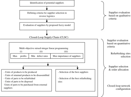
4.3. Proposed model...40
4.3.1. Evaluation of suppliers...41
4.3.2. Mathematical model for CLSC...44
4.3.3. Solution approach... 48
4.4. Numerical example...49
4.5. Conclusions...52
CHAPTER 5. A THREE-STAGE MODEL FOR CLOSED-LOOP SUPPLY CHAIN CONFIGURATION UNDER UNCERTAINTY 5.1. Introduction ………...……54
5.2. Problem definition ………...…..……..55
5.3. Proposed model……….………..……...56
5.3.1. Evaluation………..57
5.3.2. CLSC network configuration ………..………..60
5.3.3. Selection and order allocation………....63
5.4. An illustrative example………..………...67
x
5.4.2. Stage 2………..……..70
5.4.3. Stage 3………...71
5.5. Managerial insights and discussions………...……….…..72
5.5.1. Comparison between the proposed model and HOQ...72
5.5.2. Sensitivity analysis of uncertain demand………...73
5.5.3. Comparison of single and multiple sourcing policies……73
5.5.4. Sensitivity analysis of capacity……….….74
5.6. Conclusions……….…...75
CHAPTER 6. A PROPOSED MATHEMATICAL MODEL FOR CLOSED-LOOP NETWORK CONFIGURATION BASED ON PRODUCT LIFE CYCLE 6.1. Introduction...76
6.2. Problem definition...77
6.3. Proposed mathematical model...79
6.4. Computational testing...82
6.5. Sensitivity analysis...83
6.6. Extended model...86
6.7. Conclusions...89
CHAPTER 7. CONCLUSIONS AND FUTURE RESEARCH 7.1. Conclusions……….…...…..91
7.2. Future research………...…..94
APPENDICES APENDIX A. Data for the numerical example (Chapter 4)...96
APENDIX B. Data for the illustrative example (Chapter 5)...99
APENDIX C. Data for the computational testing (Chapter 6)...103
REFERENCES...106
xi
LIST OF TABLES
Table 1.1 Differences in forward and reverse logistics (Tibben-Lembke and Rogers,
2002)...2
Table 1.2 Reverse logistics costs (Tibben-Lembke and Rogers, 2002)...3
Table 1.3 Special issues in related to reverse logistics...5
Table 2.1 Classification of references based on operations research techniques...15
Table 2.2 Summary of papers about supplier selection and order allocation...17
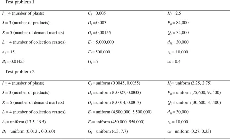
Table 3.1 Data for copier remanufacturing example...25
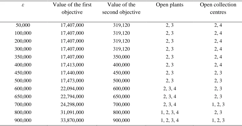
Table 3.2 Results of ε-constraint method...30
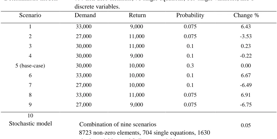
Table 3.3Scenario analysis...34
Table 4.1 Evaluation of suppliers based on qualitative criteria...51
Table 4.2 Results of CLSC configuration...52
Table 5.1The indices, parameters, and decision variables of the second and third stages...61
Table 5.2 The importance of CRs………..………68
Table 5.3 Aggregated weights………...………68
Table 5.4 Impact of customer requirements (CRs) on design requirements (DRs)…….. 68
Table 5.5 The impact of alternatives on process requirements (PRs)………69
Table 5.6 Calculating the FI and normalization….………...……...…….70
Table 5.7 Results of Stage 2………..……70
Table 5.8 Results of multi objective techniques...71
Table 5.9 Value of objective functions...72
Table 5.10 Comparison between the first stage and HOQ...72
Table 6.1 Indices, decision variables, and parameters of the proposed mathematical model………..79
Table 6.2 The computational results……….………….83
Table 6.3 Additional variables and parameters for the secondary market…………..…...87
Table A.1 Product-related parameters………...………96
xii
Table A.3 Refurbishing site-related parameters………...……….96
Table A.4 The usage of part i per unit of product j……….………….………..97
Table A.5 Supplier-related parameters………...……….…..97
Table A.6 Capacities………..98
Table B.1 Product and part related parameters……….….99
Table B.2 Remanufacturing subcontractor-related parameters………..99
Table B.3 Refurbishing site-related parameters……….……100
Table B.4 Supplier-related parameters………..………..101
Table B.5 Customer-related parameters………..………102
Table B.6 Capacities………...……….102
Table C.1 Product-related parameters………...……….103
Table C.2 Part-related parameters………..……..103
Table C.3 The usage of part i per unit of product j………..………103
Table C.4 Recycling site-related parameters………..…………...………..104
Table C.5 Supplier-related parameters………..…………..………105
xiii
LIST OF FIGURES
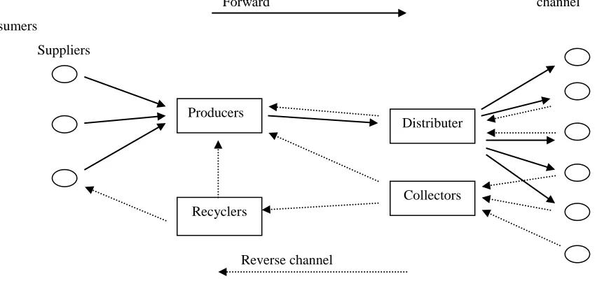
Figure 1.1. Framework of reverse distribution (Fleischmann et al., 1997)...2
Figure 1.2. The numbers of scientific articles...5
Figure 1.3. Triangular fuzzy numbers...7
Figure 1.4. Quality function deployment………...………..……8
Figure 1.5. House of quality………..…..8
Figure 2.1. Green supply chain management framework (Srivastava, 2008)...14
Figure 3.1. The closed-loop supply chain network...21
Figure 3.2. Optimal closed-loop supply chain network (test problem 1, product 2)...26
Figure 3.3. Optimal closed-loop supply chain network (test problem 2, product 2)...26
Figure 3.4. Trade-off surfaces for the test problem 2: (a) weighted sums method, (b) ε-constraint method, (c) weighted sums and ε-ε-constraint methods...29
Figure 3.5. Objective values of deterministic scenarios (1-9) and stochastic case (scenario 10)...34
Figure 3.6. Sensitivity analysis of αj in deterministic (base-case) and stochastic scenarios...35
Figure 4.1. A closes-loop supply chain (dashed area)...40
Figure 4.2. Framework of the proposed model...41
Figure 4.3. Proposed supplier selection criteria in reverse logistics...43
Figure 4.4. A linguistic scale (Amin and Razmi, 2009)...43
Figure 4.5. Supplier evaluation based on qualitative criteria...50
Figure 5.1.Framework for remanufacturing system – the dashed area (Kim et al., 2006)………..………56
Figure 5.2. Framework of the proposed model...57
Figure 5.3. A linguistic scale for triangular fuzzy numbers………..58
Figure 5.4. Qualitative criteria………..……….…68
Figure 5.5. The first matrix of QFD...69
Figure 5.6. The second matrix of QFD...70
xiv
Figure 5.8. Value ofobjective function of single and multiple sourcing policies
(compromise method)...74
Figure 5.9. Sensitivity analysis for capacity of remanufacturing subcontractors...74
Figure 6.1. A closed loop supply chain network based on product life cycle (highlighted
area)………78
Figure 6.2. Sensitivity analysis of the max capacity of disassembly site to dissemble part
1………...……….….….84
Figure 6.3. Sensitivity analysis of N (max percent of total returns)………..85
Figure 6.4. Sensitivity analysis of z (max percent of commercial returns)………85
Figure 6.5. Sensitivity analysis of M1 (max percent of end of use returns), M2 (max
percent of end of life returns………..………86
Figure 6.6. Sensitivity analysis of the max capacity of disassembly site to dissemble part
1 (secondary market)……….………….88
Figure 6.7. Sensitivity analysis of N (max percent of total returns), (secondary
market)………...88
Figure 6.8. Sensitivity analysis of z (max percent of commercial returns), (secondary
market)……… ……….….……89
Figure 6.9. Sensitivity analysis of M1 (max percent of end of use returns), M2 (max
1
CHAPTER 1. INTRODUCTION
Nowadays, supply chain management (SCM) has received a lot of attentions. In APICS
Dictionary, SCM is defined as the design, planning, execution, control, and monitoring of
supply chain activities with the objective of creating net value, building a competitive
infrastructure, leveraging worldwide logistics, synchronizing supply with demand, and
measuring performance globally. There are two types of supply chains: forward and
reverse supply chains.
1.1. Forward supply chain
The forward supply chain (FSC) includes of series of activities in the process of
converting raw materials to finished products. The managers try to improve forward
supply chain performances in areas such as demand management, procurement, and order
fulfillment (Cooper et al., 1997).
1.2. Reverse supply chain
Reverse supply chain (RSC) is defined as the activities of the collection and recovery of
product returns in supply chain management (SCM). Economic features, government
directions, and customer pressure are three aspects of reverse logistics (Melo et al., 2009).
Generally, there are more supply points than demand points in reverse logistics networks
when they are compared with forward networks (Snyder, 2006). Reverse logistics include
the process of planning, implementing and controlling the inbound flow and storage of
secondary goods and related information opposite to the traditional supply chain
directions for the purpose of recovering value and proper disposal (Fleischmann, 2001).
Figure 1.1 shows a framework of reverse logistics. Besides, the differences between
forward and reverse logistics are written in Table 1.1. In addition, Table 1.2 shows the
costs of reverse logistics and it provides a comparison between forward and reverse
2
The design of reverse logistics network is a difficult problem because of economic
aspects and the effects of it on other aspects of human life, such as the environment and
sustainability of natural resources (Lee and Dong, 2009; Francas and Minner, 2009).
Forward channel Consumers
Suppliers
Reverse channel
Figure 1.1. Framework of reverse distribution (Fleischmann et al., 1997)
Table 1.1
Differences in forward and reverse logistics (Tibben-Lembke and Rogers, 2002)
Forward Reverse
Forecasting relatively straightforward Forecasting more difficult One to many transportation Many to one transportation Product quality uniform Product quality not uniform Destination/routing clear Product packaging often damaged Standardized channel Destination/routing unclear Disposition options Exception driven
Pricing relatively uniform Disposition not clear
Importance of speed recognized Pricing dependent on many factors Forward distribution costs closely monitored by
accounting systems
Speed often not considered a priority
Inventory management consistent Reverse costs less directly visible Product lifecycle manageable Inventory management not consistent Negotiation between parties straightforward Product lifecycle issues more complex
Marketing methods well-known Negotiation complicated by additional considerations
Real-time information readily available to track product Marketing complicated by several factors Visibility of process less transparent Producers
Recyclers
3
Table 1.2
Reverse logistics costs (Tibben-Lembke and Rogers, 2002)
Cost Comparison with forward logistics
Transportation Greater
Inventory holding cost Lower
Shrinkage (theft) Much lower
Obsolescence May be higher
Collection Much higher – less standardized Sorting, quality diagnosis Much greater
Handling Much higher
Refurbishing / repackaging Significant for RL, non-existent for forward Change from book value Significant for RL, non-existent for forward
Reprocessing of used products can be efficient in (Pochampally et al., 2008):
1. Saving natural resources: We consider land and reduce the need to drill for oil and dig
for minerals by making products using materials and components obtained from
reprocessing instead of virgin materials.
2. Saving energy: It usually takes less energy to make products from reprocessed
materials and components than from virgin materials.
3. Saving clean air and water: Making products from reprocessed materials and
components create less air pollution and water pollution than from virgin materials.
4. Saving landfill space: When reprocessed materials and components are used to make a
product, they do not go into landfills.
5. Saving money: It costs much less to make products from reprocessed materials and
components than from virgin materials.
Product returns may occur for a variety of reasons over the product life cycle.
Commercial returns are products returned to the reseller by consumers within 30, 60, or
90 days after purchase. End-of-use returns occur when a functional product is replaced by
a technological upgrade. End-of-life returns are available when the product becomes
technically obsolete or no longer contains any utility for the current user. As an example,
consider the cell telephone industry. In the United States, consumers may return a mobile
phone to the airtime provider for any reason during a 30-day period after purchase (a
4
functional mobile phones annually, making their previous models available as an
end-of-use return. Finally, some end-of-users of mobile phones relinquish their phone only when it is no
longer supported by the airtime provider and it becomes available as an end-of-life return
(e.g., the technology is obsolete). There are also repair and warranty returns that occur
throughout, and even beyond, the product life cycle. It should be clear that, for consumer
electronics alone, there are billions of returned products annually in the United States,
and therefore enormous potential for value recovery (Guide and Van Wassenhove, 2009).
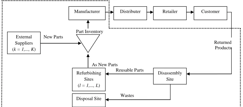
Reverse logistics options consist of reuse, resale, repair, refurbishing, remanufacturing,
cannibalization, and recycling (Thierry et al., 1995). In the remanufacturing process, used
products are disassembled in disassembly sites. Then they are divided to two kinds of
parts. Usable parts are cleaned, refurbished, and they are transmitted into part inventory.
Then the new products are manufactured from the old and new parts (Kim et al., 2006).
The purpose of refurbishing is to increase the quality of products. Quality standards are
less rigorous than those for new products. Military and commercial aircraft are examples
of these products. Although the quality of products is improved by refurbishing,
remaining service life is generally less than the average service life of new ones (Thierry
et al., 1995). For each type of product return, there is a most attractive recovery option.
Commercial returns have barely been used and are best reintroduced to the market as
quickly as possible. The majority of these returns require only light repair operations
(cleaning and cosmetic). End-of-use returns may have been used intensively over a period
of time and may therefore require more extensive remanufacturing activities. The high
variability in the use of these products may also result in very different product
disposition and remanufacturing requirements. Ideally, one would like to acquire
end-of-use products of sufficient quality to enable profitable remanufacturing. End-of-life
products are predominantly technologically obsolete and often worn out. This makes
parts recovery and recycling the only practical recovery alternatives (Guide and Van
5
1.3. Closed-loop supply chain
The integration of forward supply chain and reverse supply chain constructs a
closed-loop supply chain (CLSC) (Guide and Van Wassenhove, 2009). In other words, there are
both forward and reverse channels in CLSC networks.
Reverse logistics (RL) and closed-loop supply chain (CLSC) are the subjects of several
researches. Figure 1.2 shows the number of articles on RL and CLSC from 2000 until
beginning of 2012 which is obtained by SCOPUS. In addition, some scientific journals
have published special issues for the subject of RL. For more information, you can refer
to Table 1.3. These evidences show that a lot of researchers are working on RL and
CLSC subjects. Furthermore, these fields of study have a lot of opportunities for future
research.
Figure. 1.2. The numbers of scientific articles are identified by a search of “reverse logistics” or
“closed-loop supply chain” from 2000 to 2012. The search was performed on SCOPUS on 21 February 2012.
Table 1.3
Special issues in related to reverse logistics
Journal Subject Year Volume Issue
Interfaces Closed-loop supply chain 2003 33 6 California Management Review Closed-loop supply chain 2004 46 2 Production & Operations Management Closed-loop supply chain 2006 15 3 & 4 Computers & Operations Research Reverse logistics 2007 34 2 Journal of Operations Management SCM in a sustainable environment 2007 25 6
0 50 100 150 200 250 300 350 400 450 500
2000 2002 2004 2006 2008 2010 2012
Number of articles
6
1.4. Research objectives
The objective of this dissertation is to develop effective approaches to support
closed-loop supply chain configurations and analyses especially develop methodologies to
examine impacts of the following issues on CLSC:
Uncertainty: In the mathematical models, there are several parameters such as cost,
demand, and return which are not deterministic. As a result, several sources of
uncertainty should be considered.
Multi-objectives: In closed-loop network configuration, not only it is preferred to
minimize the total cost (including operation, transportation, and holding costs), but also it
is necessary to optimize other factors such as recycling materials and wastes because of
environmental concerns. In addition, different criteria should be considered in selection
of members of supply chain (such as suppliers). As a consequence, multi-objective
models should be proposed and appropriate solution approaches should be developed.
1.5. Solution methodologies
In this section, some important approaches are mentioned. These tools are applied in
this dissertation.
Mixed-integer linear programming: A mixed-integer linear program is the
minimization or maximization of a linear function subject to linear constraints. There are
two kinds of variables including nonnegative and integer variables in this problem.
Binary variables are special case of integer variables that can be 0 or 1.
Multi-objective programming: Multi objective optimization allows a degree of freedom
which is lacking in mono objective optimization. The flexibility is not without
consequences for the method used to find an optimum for the problem when it is finally
modelled. The search will give us not a unique solution but a set of solutions. These
solutions are called Pareto solutions, and the set of solutions that we find at the end of
7
Stochastic programming: The goal of stochastic optimization is to find a solution that
will perform well under any possiblerealization of the random parameters.The objective
functions of many of stochastic models are minimization of the expected cost or
maximization of theexpected profit of the system (Snyder, 2006).
Fuzzy sets theory: The term fuzzy was proposed by Zadeh (1965). The fuzzy sets theory
(FST) is introduced to improve the oversimplified model by developing a more robust
and flexible model in order to solve real-world complex systems involving human aspects
(Lai and Hwang, 1995). In addition, FST can help us to overcome uncertainty in human
thought. A fuzzy number is illustrated by membership function that is a number between
0 and 1.
Triangular fuzzy number (TFN) is one of the most important fuzzy numbers. TFNs can
be denoted as X = (a, n, b) and Y = (c, m, d), where n and m are the central values, a and
c are the left spreads, and b and d are the right spreads (see Figure 1.3). Then C = (a+c,
n+m, b+d) is the addition of these two numbers. Besides, D = (a-c, n-m, b-d) is the
subtraction of them. Moreover, is the multiplication of them (Lai
and Hwang, 1995; Zimmermann, 2001).
μ 1
a n b c m d
Figure 1.3. Triangular fuzzy numbers
µX (x) =
b n n x b
x b
,
n x a a n
a
x
,
a x ,
0
b x ,
0
) , ,
(a c n mb d
8
Quality function deployment (QFD) is a useful method that frequently is utilized in
design quality. QFD is a unique method that can consider the relationship between
elements such as customer and design requirements. QFD also is helpful in selection
problems. Figure 1.4 displays a typical QFD. Besides, the first matrix of QFD which is
called house of quality (HOQ) is illustrated in Figure 1.5. Bevilacqua et al. (2006) used
HOQ for supplier selection. However, they did not take into account quantitative factors
such as on-time delivery. Amin and Razmi (2009) combined a quantitative method with
HOQ to take into account qualitative and quantitative metrics to select the best internet
service provider.
Figure. 1.4. Quality function deployment including customer requirements (CRs), design requirements
(DRs), parts requirements (PRs), process operations (POs), and production characteristics (PCs)
Figure. 1.5. House of quality
1.6. Organization of the dissertation
The dissertation is arranged as follows: Chapter 2 presents review of literature. In
Chapter 3, a facility location model for closed-loop supply chain network is discussed.
Then, an integrated model for closed-loop supply chain configuration and supplier
selection is proposed in Chapter 4. Chapter 5 presents a three-stage model for closed-loop
supply chain configuration under uncertainty. A mathematical model is proposed based
on product life cycle in Chapter 6. Finally, Chapter 7 presents conclusions and future
works.
(A) Customer requirements (CRs) (B) Prioritized CRs
(C) Design requirements (DRs) (D) Relationship between CRs and DRs (E) Interrelationship between DRs (F) Prioritized technical descriptors
(E)
(C)
(D) (B)
(A)
(F)
Phase 1 DRs Phase 2 PRs Phase 3 POs Phase 4
CRs
9
CHAPTER 2. REVIEW OF LITERATURE
Several papers have been published about reverse logistics and closed-loop supply
chain networks. Fleischmann et al. (1997) presented a literature review for RL. They
examined the related papers based on three main categories including distribution
planning, inventory, and production planning. Rubio et al. (2008) presented a literature
review of the papers on RL published in the scientific journals within the period
1995-2005. Melo et al. (2009) presented a literature review for the application of facility
location models in supply chain management. They stated that the goal of the majority of
models is to determine the network configuration by minimizing the total cost. However,
profit maximization and multiple objectives have received less attention. Moreover, they
implied that a few papers use stochastic parameters combined with other aspects such as
multi-layer network structure. Guide and Van Wassenhove (2009) stated that the
evolution of closed-loop supply chain networks can be examined in five phases including
the golden age of remanufacturing, reverse logistics process, coordinating the reverse
supply chain, closing the loop, and prices and markets. Pokharel and Mutha (2009)
reviewed articles of reverse logistics. They stated that it is useful to develop pricing
models for acquiring used products. It is also mentioned that a limited articles have taken
into account stochastic demand of new products and supply of used-products. Akcali and
Cetinkaya (2011) provided literature review and survey for the papers of RL and CLSC.
2.1. Deterministic models for closed-loop supply chains
Network configuration is one of the main research streams in RL. The majority of
authors use facility location models to formulate CLSC networks. Jayaraman et al. (1999)
proposed a mixed-integer programming model. The model can determine the location of
remanufacturing /distribution facilities, the transhipment, production, and stocking of the
optimal quantities of remanufactured products and used parts. Fleischmann et al. (2001)
proposed a general model for closed-loop supply chain network. The model is designed
based on forward facility location model. Copier remanufacturing and paper recycling are
utilized to show the efficiency of the model. Kim et al. (2006) configured a general CLSC
10
returned products from customers. Then, they are collected in the collection site. The
returned products are disassembled. The products that are beyond the capacity of
disassembly site are sent to the remanufacturing subcontractor. The disassembled parts
are categorized to reusable parts and wastes. The reusable parts are carried to the
refurbishing site to be cleaned and repaired. Then, according to the number of refurbished
and remanufactured parts, new parts are purchased from external supplier. Lu and Bostel
(2007) presented a two-level location problem with three types of facility to be located in
a specific reverse logistics system. They proposed a mixed-integer programming model,
in which simultaneously consider “forward” and “reverse” flows and their mutual
interactions. They developed an algorithm based on Lagrangian heuristics. Ko and Evans
(2007) proposed a mixed-integer nonlinear programming model that is a multi period,
two-echelon, multi commodity, and capacitated network design problem. They
considered forward and reverse flows simultaneously. Srivastava (2008) proposed a
framework for analysing a network. The model determines the disposition decision for
various grades of different products concurrently with location-allocation and capacity
decisions for facilities for a time horizon. Kannan et al. (2009) designed an integrated
forward logistics multi-echelon distribution inventory supply chain model and
closed-loop multi-echelon distribution inventory supply chain model for the built-to-order
environment using genetic algorithm and particle swarm optimisation. Lee et al. (2009)
formulated a mathematical model for a general CLSC network by proposing a heuristic
approach (Genetic Algorithm). Although the model can determine the optimal numbers
of disassembly and processing centers, the supplier selection is not taken into account.
The authors supposed that there is only one supplier. Xanthopoulos and Iakovou (2009)
developed two phases model for reverse logistics. In the first phase, appropriate
components are identified by a decision making model. In the second one, a multi-period
optimization model is applied to configure the network.
Lee and Chan (2009) proposed a Genetic Algorithm to determine such locations in
order to maximize the coverage of customers. Besides, the use of RFID is suggested to
count the quantities of collected items in collection points and send the signal to the
central return center. Cruz-Rivera and Ertel (2009) modelled a reverse logistics network
11
using software. Furthermore, they presented a brief description of the current Mexican
ELV management system and the future trends in ELV generation in Mexico. Wang and
Hsu (2010) investigated the integration of forward and reverse logistics, and they
proposed a generalized closed-loop model for the logistics planning by formulating a
cyclic logistics network problem into an integer linear programming model. Moreover,
the decisions for selecting the places of factories, distribution centers, and dismantlers
with the respective operation units were supported with the minimum cost. They also
developed a revised spanning-tree based genetic algorithm. Kannan et al. (2010)
developed a multi echelon, multi period, multi product closed-loop supply chain network
model for product returns and the decisions are made regarding material procurement,
production, distribution, recycling and disposal. The proposed heuristics based Genetic
Algorithm is applied as a solution methodology. Achillas et al. (2010) presented a
decision support tool for policy-makers and regulators to optimise electronic products’
reverse logistics network. To that effect, they formulated a mixed-integer linear
programming mathematical model taking into account existing infrastructure of
collection points and recycling facilities. Sasikumar et al. (2010) developed a
mixed-integer nonlinear programming model for maximizing the profit of a multi-echelon
reverse logistics network and also presented a real-life case study of truck tire
remanufacturing for the secondary market segment. The proposed model is solved using
LINGO.
2.2. Uncertain models for closed-loop supply chains
Several investigations have been conducted about CLSC configuration. In the majority
of them, the parameters are deterministic (such as Kim et al., 2006). In addition, some of
authors considered uncertainty (e.g. Listes, 2007). However, the minority of them are
taken into account two or more sources of uncertainty (Snyder, 2006; Peidro et al., 2009).
Uncertainties in supply and demand are two main sources of uncertainty in SCM.
Uncertainty in supply is appeared because of the faults or delays in the supplier’s
deliveries. On the other hand, demand uncertainty is defined as inexact forecasting
demands or as volatility demands. Therefore, it is crucial to take into account uncertain
12
Peidro et al., 2009). Peidro et al. (2009) identified three dimensions of uncertainty in
supply chain management: the source of uncertainty (demand, supply, process), the
problem type (strategic, tactical, operational), and the modelling approach (analytical,
artificial intelligence-based, simulation, hybrid approaches). Inderfurth (2005) examined
a closed-loop supply chain network by stochastic programming. They considered
uncertainty in demand and return. In addition, they defined a parameter to measure
uncertainty in quality. Listes (2007) proposed a stochastic model for the design of
networks including both supply and return channels in a CLSC. They described a
decomposition approach for solving the model based on the branch-and-cut method.
Salema et al. (2007) presented a general model for reverse logistics network when there
are capacity limits, and uncertain demands and returns. Lieckens and Vandaele (2007)
proposed a mixed-integer nonlinear programming model based on queuing theory and
stochastic lead time. However, it is designed for a single product. Selim and Ozkarahan
(2008) developed a fuzzy goal programming approach for a reverse logistics network.
The uncertainty in demand and decision makers’ (DM) aspiration levels for the goals are
taken into account. Francas and Minner (2009) studied the network design problem of a
company that manufactures new products and remanufactures returned products in its
facilities. They examined the capacity decisions and expected performance of
manufacturing network configurations under uncertain demand and return. Pishvaee et al.
(2009) proposed a deterministic optimization model for a reverse logistics network. Then,
a scenario-based stochastic model is developed. Qin and Ji (2010) configured a reverse
logistics network by three kinds of mathematical models. In the first and second ones,
expected cost and α-cost are minimised, respectively. In addition, in the third one,
credibility is maximized. The unique feature of this paper is that costs and return are
triangular fuzzy numbers. The authors proposed fuzzy simulation and Genetic Algorithm
to solve the model. El-Sayed et al. (2010) developed a stochastic model for a generic
closed-loop network. It is supposed that demand is an uncertain parameter. In addition,
the model is designed for multi-periods. They considered uncertainty in demand, return,
and cost. Shi et al. (2010) proposed a mathematical model to maximize the profit of a
remanufacturing system by developing a solution approach based on Lagrangian
13
studied a production planning problem for a multi-product closed-loop system. The
authors considered uncertain demand and return by stochastic programming. Pishvaee et
al. (2011) proposed a deterministic mixed-integer linear programming model for a
closed-loop supply chain network. Then, robust optimization has been applied for the
model to consider uncertainty.
2.3. Multi-objective models for closed-loop supply chains
Some authors have used multi-objective and goal programming models to formulate
closed-loop supply chain networks. One objective can be minimizing the total cost.
Besides, because of importance of environmental issues, some objective functions may be
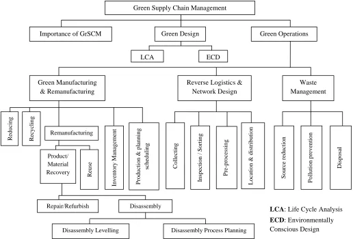
added. Figure 2.1 shows a classification of green supply chain management and
importance of green operations in reverse logistics. Krikke et al. (2003) developed
quantitative modelling to support decision-making concerning both the design structure
of a product, i.e. modularity, reparability and recyclability, and the design structure of the
logistic network. Environmental impacts are measured by linear-energy and waste
functions. They applied to a closed-loop supply chain design problem for refrigerators
using real life R & D data of a Japanese consumer electronics company concerning its
European operations. The objectives are minimization of the supply chain costs, energy
use, and residual waste. Sheu et al. (2005) proposed a linear multi-objective programming
model that systematically optimizes the operations of both integrated logistics and
corresponding used-product reverse logistics in a given green-supply chain. Factors such
as the used-product return ratio and corresponding subsidies from governmental
organizations for reverse logistics are considered in the model formulation. The
objectives are maximization of the manufacturing chain-based net profit, and the reverse
chain-based net profit. Uster et al. (2007) considered a multi-product closed-loop supply
chain network design problem where they located collection centers and remanufacturing
facilities while coordinating the forward and reverse flows in the network so as to
minimize the processing, transportation, and fixed location costs. They utilized Benders
decomposition approach to solve the model. Demirel and Gokcen (2008) presented a
mixed-integer mathematical model for a remanufacturing system, which includes both
14
formulated a mixed-integer goal programming model to determine the facility location,
route and flow of different varieties of recyclable wastepaper in the item,
multi-echelon and multi-facility decision making framework. In the paper of Du and Evans
(2008), a bi-objective optimization model is proposed. The objectives consist of
minimization of the total costs and minimization of the overall tardiness of cycle time.
The solution approach includes a combination of dual simplex, Scatter Search, and the
constraint method. Gupta and Evans (2009) proposed a non-preemptive goal
programming approach to model a closed-loop supply chain network. Pishvaee et al.
(2010) developed a bi-objective mixed-integer programming model. The first objective
minimizes the total costs and the second one maximizes the responsiveness of a logistics
network. Then, the problem has been solved by Memetic Algorithm.
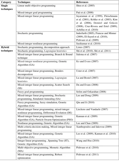
Table 2.1 shows classification of closed-loop network configuration references based
on operations research techniques.
Figure 2.1. Green supply chain management framework (Srivastava, 2008)
Green Supply Chain Management
Green Operations Importance of GrSCM Green Design
LCA ECD
Green Manufacturing & Remanufacturing
Reverse Logistics & Network Design Waste Management Re d u cin g Re cy cli n g Remanufacturing Product/ Material Recovery Reu
se In v en to ry M an ag em en t P ro d u cti o n & p lan n in g sc h ed u li n g Co ll ec ti n g In sp ec ti o n / S o rti n g P re -p ro ce ss in g Lo ca ti o n & d istri b u ti o n S o u rc e re d u cti o n P o ll u ti o n p re v en ti o n Disp o sa l
Repair/Refurbish Disassembly
Disassembly Levelling Disassembly Process Planning
LCA: Life Cycle Analysis
15
Table 2.1
Classification of references based on operations research techniques
Category Techniques References
Single techniques
Linear multi-objective programming Sheu et al. (2005)
Mixed-integer goal programming Pati et al. (2008)
Mixed-integer linear programming Jayaraman et al. (1999), Fleischmann et al. (2001), Krikke et al. (2003), Kim et al. (2006), Demirel and Gokcen
(2008), Cruz-Rivera and Ertel (2009), Achillas et al. (2010)
Stochastic programming Inderfurth (2005), Francas and Minner (2009), El-Sayed et al. (2010), Pishvaee et al. (2009)
Mixed-integer nonlinear programming Sasikumar et al. (2010)
Hybrid techniques
Stochastic programming, decomposition approach Listes (2007)
Stochastic programming, Lagrangian heuristics Shi et al. (2010), Shi et al. (2011) Mixed-integer linear programming, Branch & Bound
technique
Salema et al. (2007)
Mixed-integer nonlinear programming, Genetic
Algorithm (GA)
Ko and Evans (2007)
Mixed-integer linear programming,Benders decomposition
Uster et al. (2007)
Mixed-integer linear programming, Lagrangian heuristics
Lu and Bostel (2007)
Mixed-integer linear programming,Scatter Search (SS)
Du and Evans (2008)
Fuzzy goal programming Selim and Ozkarahan (2008) Mixed-integer linear programming, Stochastic
programming, Simulated Annealing (SA)
Lee and Dong (2009)
Fuzzy programming, fuzzy simulation, Genetic Algorithm (GA)
Qin and Ji (2010)
Mixed-integer linear programming, mixed-integer nonlinear programming, Differential Evolution (DE)
Lieckens and Vandaele (2007)
Mixed-integer linear programming, Genetic
Algorithm (GA), Particle Swarm Optimization (PSO)
Kannan et al. (2009)
Nonlinear programming, Genetic Algorithm (GA) Lee and Chan (2009) Multi-criteria decision making, Mixed-integer linear
programming
Xanthopoulos and Iakovou (2009)
Mixed-integer linear programming, Genetic Algorithm (GA)
Lee et al. (2009), Kannan et al. (2010)
Integer linear programming , Spanning Tree (ST), Genetic Algorithm (GA)
Wang and Hsu (2010)
Multi-objective programming, Memetic Algorithm (MA)
Pishvaee et al. (2010)
Mixed-integer linear programming, Robust optimization
16
2.4. Supplier selection
In the field of supplier selection and evaluation, a lot of articles have been published.
Weber et al. (1991) sent a questionnaire to several companies. They identified the most
important criteria including price, delivery, quality, facilities, geographic location, and
technology. De Boer et al. (2001) presented a literature review for all phases in the
supplier selection process from initial problem definition, over the formulation of criteria,
the qualification of potential suppliers, and final choice among the qualified suppliers.
Humphreys et al. (2003) presented a new framework to select the best suppliers based on
environmental criteria such as solid waste, chemical waste, air emission, water waste
disposal, and energy. Hsu and Hu (2009) presented an analytic network process model to
incorporate the issue of hazardous substance management into supplier evaluation.
Aissaoui et al. (2007) presented a literature review especially on the final selection stage
that consists of two sections: determining the best vendors, and allocating orders among
them. Recently, Ho et al. (2010) have reviewed the literature of the multi-criteria decision
making approaches for supplier selection and evaluation. They focused on the papers
from 2000 to 2008.
Some researchers have investigated application of fuzzy sets theory in supplier
selection. For instance, Bottani and Rizzi (2006) applied fuzzy TOPSIS for selecting the
best suppliers. Besides, Chan and Kumar (2007) used fuzzy AHP method. Chou and
Chang (2008) presented a strategy-aligned fuzzy approach for solving the vendor
selection problem from the strategic management view point. Their method is designed
based on operations management and triangular fuzzy numbers. Wang et al. (2009)
combined fuzzy TOPSIS and AHP methods to select the best suppliers. Amin and Razmi
(2009) proposed a general framework for supplier selection, evaluation, and
development. In addition, they applied a fuzzy-QFD based algorithm for selecting the
best internet service provider (ISP).
Ghodsypour and O’Brien (1998) proposed a new model to select the best supplier and
determine the order allocation. They used analytical hierarchy process (AHP) to consider
qualitative criteria. On the other hand, linear programming (single objective) was utilized
to take into account quantitative metrics. After this paper, a lot of investigations have
17
formulated as multi-objective programming, because it is desirable to maximize and
minimize some objective functions, simultaneously. The main differences between these
papers are related to the application of decision techniques. However, all of them are
written for open loop supply chain networks. In addition, the majority of them only are
examined constraints of demand and capacity of suppliers. On the other hand, one of the
key elements of closed-loop supply networks is external supplier. To date, suppliers are
selected based on single criterion (purchasing cost) in closed-loop supply chain networks.
But, other factors such as quality and delivery and responsiveness of suppliers also are
essential.
Table 2.2
Summary of some papers about supplier selection and order allocation
Authors Supplier selection techniques Order allocation techniques
Ghodsypour and O’Brien (1998) Analytical hierarchy process (AHP) Linear programming Xia and Wu (2007) AHP and rough sets theory Mixed-integer programming Ustun and Demirtas (2008) ANP Goal programming
Sanayei et al. (2008) Utility theory Linear programming Lin (2009) Fuzzy preference programming Linear programming Demirtas and Ustun (2009) ANP Goal programming
Wu et al. (2009) ANP Mixed-integer programming
Faez et al. (2009) Fuzzy case-based reasoning Mixed-integer programming Razmi et al. (2009)
Amin et al. (2011)
Fuzzy
Fuzzy SWOT analysis
Fuzzy linear programming Fuzzy linear programming
2.5. Potential future research
The potential future researches based on literature survey are as follows:
1- In closed-loop network configuration, not only it is preferred to minimize the total cost
(including operation, transportation, and holding costs), but also it is necessary to
optimize other factors such as recycling materials and wastes because of environmental
concerns. In addition, different criteria should be considered in selection of members of
supply chain (such as suppliers). As a consequence, multi-objective models should be
18
2- Another problem is related to the uncertainty. In the mathematical models, there are
several parameters such as cost, demand, and return which are not deterministic. As a
result, several sources of uncertainty should be considered. To this aim, some techniques
such as fuzzy sets theory, stochastic programming, and robust optimization can be
applied.
3- The minority of authors have taken into account multi-objective closed-loop supply
chain models under uncertainty. It is valuable to examine integrated models including
multi-objective and uncertainty.
4- There are several types of costs in reverse logistics such as transportation, inventory,
shrinkage (theft), obsolescence, collection, sorting, quality diagnosis, handling,
repackaging, and change from book value. In the majority of models, authors have
considered only some of these costs. It is worthwhile to take into account a collection of
them.
5- Another issue is the complexity of mathematical models. The complexity of network
leads to large mathematical models that cannot be solved quickly by commercial software
such as GAMS. Therefore, heuristic and meta-heuristics algorithms such as Scatter
Search should be proposed.
6- The most of proposed closed-loop supply chain models have not considered
multi-period inventory management parameters. In this situation, the inventory and related
holding costs should be calculated.
7- The most of closed-loop supply chain models are mixed-integer linear programming
models. There are some techniques such as Branch & Bound and Benders decomposition
approach to calculate exact solutions. The application of these techniques and designing
efficient solution algorithms can be subject of future research.
19
CHAPTER 3. A MULTI-OBJECTIVE FACILITY LOCATION
MODEL FOR CLOSED-LOOP SUPPLY CHAIN NETWORK UNDER
UNCERTAIN DEMAND AND RETURN
3.1. Introduction
Supply chain management (SCM) has received a lot of attentions. There are two types
of supply chains: forward and reverse supply chains. The forward supply chain (FSC)
contains of series of activities which result in the conversion of raw materials to finished
products. Managers try to improve forward supply chain performances in areas such as
demand management, procurement, and order fulfilment (Cooper et al., 1997). Reverse
supply chain (RSC) is defined as the activities of the collection and recovery of product
returns in SCM. Economic features, government directions, and customer pressure are
three aspects of reverse logistics (Melo et al., 2009). The integration of a forward supply
chain and a reverse supply chain results in a closed-loop supply chain (CLSC) (Guide and
Van Wassenhove, 2009). In other words, there are both forward and reverse channels in
CLSC networks.
Several investigations have been done about forward facility location models. Facility
location models try to answer the following questions: How many facilities should be
open? Where each facility should be located? What is the allocation? Which set of
collection centres should be opened and operated? What products should be processed in
these open facilities? Some authors have examined facility location models for
closed-loop supply chain networks (such as Fleischmann et al., 2001). The objective of these
models is to determine decision variables of both forward and reverse channels.
Minimization of total cost is considered as main objective function. A minority of authors
not only considered the total cost, but also they took into account other factors by
multi-objective models. On the other hand, some researchers investigated uncertainty in CLSC
configuration (for instance Salema et al., 2007). Uncertainties in supply and demand are
two major sources of vagueness in SCM. Uncertainty in supply is appeared because of
the mistakes or delays in the supplier’s deliveries. Demand uncertainty is defined as
inexact forecasting demands or as volatility demands (Davis, 1993; Snyder, 2006; Zhang
20
logistics. To our knowledge, most of authors have not taken into account multi-objective
closed-loop supply chain models under uncertainty. Thus, it is valuable to examine
integrated models including multi-objective models with uncertain parameters.
In this chapter, a facility location model is proposed for a general closed-loop supply
chain network. The model is designed for multiple plants (manufacturing and
remanufacturing), demand markets, collection centres, and products. The goal is to know
how many and which plants and collection centres should be open, and which products
and in which quantities should be stock in them. The objective function minimizes the
total cost. In this chapter, two test problems are examined. In addition, the model is
developed to multi-objective by considering environmental factors. Then, it is solved by
two methods including weighted sums and ε-constraint methods. Furthermore, trade-off
surfaces of test problems are examined. The multi-objective model also is extended by
stochastic programming (scenario-based) to examine the effects of uncertain demand and
return on the network configuration. Finally, computational results are discussed and
analysed. This research is among the first investigations that consider multi-objective
mathematical models under uncertainty in CLSC network configuration.
The organization of this chapter is as follows. In Section 3.2, a general network is
described. In Section 3.3, the mathematical model is provided. Then, two test problems
are presented in Section 3.4. An extension to multi-objective programming is provided in
Section 3.5. In addition, the model is developed by stochastic programming in Section
3.6. Finally, conclusions are discussed in Section 3.7.
3.2. Network description
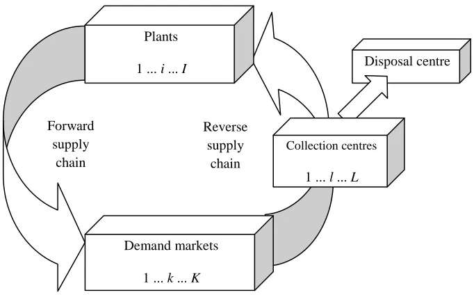
In this section, a general closed-loop supply chain network is described. Figure 3.1
shows the network which includes plants, collection centres, and demand markets. The
plants can manufacture new products and remanufacture returned products. The products
are sent to demand markets by plants. Then, the returned products are sent to collection
centres. Collection centres have the following responsibilities: collecting of used products
from demand markets, determining the condition of the returns by inspection and/or
separation to find out whether they are recoverable or not, sending recoverable returns to
21
reasons) to the disposal centre. The objective is to know how many and which plants and
collection centres should be open, and which products and in which quantities should be
stock in them.
The following assumptions are made in the network configuration:
All of the returned products from demand markets are collected in collection
centres.
Locations of demand markets are fixed.
Locations and capacities of plants and collection centres are known in advance.
Figure 3.1. The closed-loop supply chain network
3.3. Mathematical model
The network can be formulated as a mixed-integer linear programming model. Sets,
parameters, and decision variables are defined as follows:
Sets
I = set of potential manufacturing and remanufacturing plants locations (1 ... i ... I)
J = set of products (1 ... j ... J)
K = set of demand markets locations (1 ... k ... K)
L = set of potential collection centres locations (1 ... l ... L)
Forward supply
chain
Plants
1 ... i ... I Disposal centre
Collection centres
1 ... l ... L
Reverse supply
chain
22
Parameters
Aj = production cost of product j
Bj = transportation cost of product j per km between plants and demand markets
Cj = transportation cost of product j per km between demand markets and collection
centres
Dj = transportation cost of product j per km between collection centres and plants
Oj = transportation cost of product j per km between collection centres and disposal
centre
Ei = fixed cost for opening plant i
Fl = fixed cost for opening collection centre l
Gj = cost saving of product j (because of product recovery)
Hj = disposal cost of product j
Pij = capacity of plant i for product j
Qlj = capacity of collection centre l for product j
tik = the distance between location i and k generated based on the Euclidean method (tkl
and tli are defined in the same way). tl is the distance between collection centre l and
disposal centre
dkj = demand of customer k for product j
rkj = return of customer k for product j
αj = minimum disposal fraction of product j
Variables
Xikj = quantity of product j produced by plant i for demand market k
Yklj = quantity of returned product j from demand market k to collection centre l
Slij = quantity of returned product j from collection centre l to plant i
Tlj = quantity of returned product j from collection centre l to disposal centre
Zi = 1, if a plant is located and set up at potential site i, 0, otherwise
Wl = 1, if a collection centre is located and set up at potential site l, 0, otherwise
l lj j l j j l lij i j li j jk l j
klj kl j
i k j
23 s.t.
The objective function is minimization of the total cost. The first and second parts show
the fixed costs of opening plants and collection centres, respectively. The third part
represents the production and transportation costs of new products. The forth part is
related to product recovery and transportation costs of returned products. Besides, the
fifth part represents the total recovery and transportation costs of returned products from
collection centres to plants. Besides, the sixth part calculates disposal and transportation
costs.
The constraint (3.1) ensures that the total number of each product for each demand
market is equal or greater than the demand. Constraint (3.2) is a capacity constraint of
plants. Constraint (3.3) represents that forward flow is greater than reverse flow.
Constraint (3.4) enforces a minimum disposal fraction for each product. Constraint (3.5) ) 1 . 3 ( , ,j k d X kj i
ikj
) 7 . 3 ( , ,j k r Y kj lklj
) 3 . 3 ( , , j k X Y i ikj lklj
) 4 . 3 ( , ,j l T Y lj k kljj
) 2 . 3 ( , i P Z X S j ij i k j ikj l j
lij
) 5 . 3 ( , l Q W Y j lj l k jklj
0,1 , , (3.8),W i l
Zi l
) 9 . 3 ( , , , , 0 , ,
,Y S T i k l j
Xikj klj lij lj
) 6 . 3 ( , ,j l T S Y lj i lij k
klj