ABSTRACT
MAYUKH, HIRAN. FabIssue: Automatic RTL Generation of Issue Logic in Superscalar Processors for Core Customization. (Under the direction of Dr. Eric Rotenberg.)
FabIssue: Automatic RTL Generation of Issue Logic in Superscalar Processors for Core Customization
by Hiran Mayukh
A thesis submitted to the Graduate Faculty of North Carolina State University
in partial fulfillment of the requirements for the degree of
Master of Science
Computer Engineering
Raleigh, North Carolina 2010
APPROVED BY:
_______________________________ ______________________________ Dr. Eric Rotenberg Dr. James Tuck
Committee Chair
DEDICATION
BIOGRAPHY
ACKNOWLEDGMENTS
I would like to express my gratitude to Prof. Eric Rotenberg for inspiring and guiding me throughout the duration of my masters at N.C. State. He is a wonderful teacher and it has been an honor working with him. I thank Prof. James Tuck and Prof. Huiyang Zhou for their support. This thesis would not have been possible without the work of Niket Choudhary, Salil Wadhavkar, Sandeep Navada, Jayneel Gandhi, Tanmay Shah and Hashem Hashemi – you guys are awesome. Thanks to Naser Sedaghati, Rami Al-Sheikh, Julian and others at CESR, my apartment-mates Sounder Rajan Vijay Kumar, Suhas Satish and Abhinav Naik, and my family for all the support and encouragement.
TABLE OF CONTENTS
LIST OF TABLES ... vii
LIST OF FIGURES ... viii
1. Introduction ... 1
1.1. Issue Logic and Performance ... 2
1.2. Contribution ... 4
2. Motivation ... 6
2.1. Tradeoffs in Issue Logic Design ... 8
2.1.1. Issue Width ... 9
2.1.2. Issue Queue Size ... 9
2.1.3. Issue Depth... 10
2.2. Heterogeneity and Core Customization ... 14
2.3. FabIssue ... 17
3. Related Work ... 19
3.1. Issue Logic ... 19
3.2. Design and Performance ... 19
3.3. Simulators ... 20
3.4. FabScalar... 21
. 4. Design of the Issue Logic ... 23
4.1. Working of the Issue Logic... 24
4.1.1. Dispatching an Instruction ... 25
4.1.2. Generation of Request Vectors ... 25
4.1.3. Select Logic ... 26
4.1.4. Wakeup CAM ... 30
4.1.5. Result Shift Register ... 30
4.1.6. Wakeup-Select Loop ... 31
4.1.7. Free List Management ... 34
4.1.8. Cascaded Select trees ... 34
4.2. Pipelining the Issue Logic ... 36
4.2.1. The 1/1 Issue Logic Configuration ... 36
4.2.2. The 2/2 Issue Logic Configuration ... 37
4.2.3. The 3/3 Issue Logic Configuration ... 38
4.2.4. The 2/3 Issue Logic Configuration ... 39
4.2.5 Pipelining the Select Logic ... 40
5. FabIssue ... 42
6. Methodology ... 45
6.1. Experiments ... 45
6.2. Assumptions and Limitations ... 46
7.1. Issue Queue Configuration and Performance ... 50
7.2. Diversity across benchmarks ... 52
7.3. Diversity within a benchmark ... 52
7.4. Understanding Diversity Results ... 54
7.4.1. Lack of Diversity in Issue Depth ... 54
7.4.2. Lack of Diversity in Issue Width ... 55
7.4.3. Understanding the Best Issue Logic Configuration ... 56
7.4.4. Eliminating Issue Logic Configurations ... 59
7.5. Can the Best Configuration be Wide or Shallow? ... 61
8. Conclusion ... 63
8.1. Summary of Results ... 64
LIST OF TABLES
Table 4.1. Instruction types in FabScalar and their execution latencies. ... 34
Table 5.1. Parameterized processor attributes in FabScalar.. ... 42
Table 5.2. Script call flow in FabScalar. ... 44
Table 6.1. Benchmarks, input arguments and run starting points ... 48
Table 6.2. Configuration of the processor ... 49
Table 7.1. Performance (IPT) results in BIPS for all benchmarks run across all issue logic configurations tested. ... 50
Table 7.2. Cycle time of configurations A and B as a function of components of the issue logic... 57
Table 7.3. Elimination of issue logic configurations by finding another configuration that always performs better.. ... 60
LIST OF FIGURES
Figure 2.1. Running a workload having serially-dependent chain of instructions on a
machine with issue logic sub-pipelined into two stages. ... 12
Figure 2.2. Running a workload having serially-dependent chain of instructions on a machine with unpipelined issue logic.. ... 13
Figure 3.1. Canonical Pipeline stages in FabScalar ... 22
Figure 4.1. Components of the Issue Logic ... 24
Figure 4.2. 4:1 select block. grantIn comes from the next level of the select tree. ... 28
Figure 4.3. Portion of a 16:1 select logic built out of 4:1 select blocks. ... 29
Figure 4.4. The issue logic shown with the wakeup-select loop highlighted ... 32
Figure 4.5. 1/1 issue logic configuration... 37
Figure 4.6. 2/2 issue logic configuration... 38
Figure 4.7. 3/3 issue logic configuration... 39
Figure 4.8. 2/3 issue logic configuration... 40
1. Introduction
Superscalar processors fetch and execute multiple instructions each cycle. This is in
contrast with scalar processors, which execute a maximum of one instruction per
cycle - hence the qualifier 'super.' The move from scalar to superscalar processors
to achieve higher instruction throughput is made possible by the independence that
exists between instructions, which allows multiple instructions to execute in parallel
(at the same time) without being incorrect. This parallelism present among
instructions is known as instruction-level parallelism or ILP.
A modern out-of-order superscalar processor can be thought of as consisting of two
parts, the front-end and the back-end. The front-end fetches multiple instructions in
program order, renames the source and destination registers to eliminate false
dependencies, and places instructions in the issue queue. The back-end polls the
readiness of instructions in the issue queue, and selects multiple ready-to-execute
instructions to be sent out of program order down the back-end pipeline stages
where the instructions are executed. The final stage of the backend updates the
architectural state of the machine in program order.
An instruction in the issue queue is said to be ready in a certain cycle if the
instruction‟s source operand values are available or expected to be available, so that
issuing the instruction in that cycle (or later) results in correct execution. To achieve
of instructions must execute each cycle, and hence, a large number of ready
instructions must be available each cycle in the issue queue. Achieving this is
challenging because data dependencies exist between instructions – dependent
instructions will not become ready until the issue of instruction(s) producing its
source operand values. To overcome the problem of data dependencies limiting
available ILP and throttling instruction throughput, the front-end speculates past
branches (via branch prediction). The issue queue can then build a large pool of
instructions that enables looking far ahead in the program in search for independent
(and hence, ready) instructions.
Instructions in the issue queue are polled for readiness each cycle and a sub-set of
ready instructions are selected and granted permission to issue (the select process).
These instructions are sent in parallel to the function units (the issue process). The
issue logic also ensures that instructions in the issue queue become ready at the
earliest possible time without compromising correctness (the wakeup process).
The part of the processor that handles the wakeup, select and issue processes is
called the issue logic. This thesis deals with the issue logic and the effect of its
configuration on program performance.
1.1. Issue Logic and Performance
The issue logic can be characterized by three parameters – issue width, issue queue
a) Issue width is the maximum number of instructions that can be issued in a
cycle.
b) Issue queue size is the maximum number of instructions that can be held by
the issue queue.
c) Issue depth is the degree of pipelining of the issue logic. It is the minimum
number of cycles an instruction has to spend in the issue stage.
The issue logic configuration for highest performance (defined as instructions per
unit time or IPT) is a sweet-spot in the trade-off between IPC and processor
frequency. Increasing the issue width and issue queue size allows the processor to
exploit more ILP and increase IPC. It also entails increasing structure sizes and
using longer wires, thus degrading frequency. Increasing the issue depth can
provide a higher frequency but IPC may be degraded due to the extra sub-pipeline
stages added. The relationship between issue logic configuration and performance
is, therefore, a complex one.
Studying the exact nature of the above relationship is challenging, partly due to the
definition of performance as IPT. Unlike IPC, which can be easily obtained by
simulation on cycle-accurate simulators, timing information (i.e., frequency) is highly
dependent on the exact physical design of the processor. Hence, estimation of
performance of a single issue logic configuration for a specific workload requires a
detailed design of that issue logic configuration. (Alternatives to this approach are
Furthermore, such a study would also require the ability to estimate performance for
many issue logic configurations, and hence, require a library of detailed issue logic
designs or a method to generate them automatically. This thesis follows the latter
approach.
1.2. Contribution
a) This thesis aims to understand how workload characteristics, issue logic
configuration and technology influence performance: For a given workload
and technology, what factors cause one issue logic configuration to perform
better than the other?
b) This thesis also explores program diversity within a benchmark suite in order
to ascertain the performance benefit of customizing issue logic to program
behavior: Is there enough diversity in workload characteristics so that the best
issue logic configurations differ for different workloads? If so, how much do
they differ in performance over the single best issue logic configuration for the
entire workload set? What is the performance benefit of customizing issue
logic to different program behavior in a heterogeneous multicore processor?
c) This thesis contributes FabIssue, a tool capable of generating synthesizable
RTL designs for arbitrary issue logic configurations. The designs generated
by the tool are used for both running benchmarks (gives IPC) and synthesis
The FabIssue tool has been developed as a part of the FabScalar [2] research
project, which is a collaborative effort by many students over the past two years.
Details of the FabScalar project are described in this thesis in order to bring out the
context of this work, but parts not directly related to the work in this thesis are
2. Motivation
Performance in computer architecture is the average number of instructions
committed per unit time (IPT). IPT is the product of average number of instructions
committed per cycle (IPC) and frequency. Modern out-of-order superscalar
processors achieve high IPC by exploiting instruction-level parallelism (ILP). Use of
aggressive and accurate branch prediction to speculate past branches enables
construction of a large instruction window that looks far ahead into the program in
search of independent instructions that are issued and executed in parallel. Thus,
going wider and larger translates to higher IPC. But this comes at the price of
increased complexity, since each stage of the processor handles a larger number of
instructions every cycle. There can be dependencies – data or control – among a
group of instructions in a stage, and the hardware needed to handle this correctly
brings in even more complexity. Thus, extracting higher IPC by going wider and
larger entails the use of larger, more complex logic structures, which translates to
larger logic depths and longer wire lengths, which in turn reduces the frequency at
which the processor can be clocked. This effect of complexity on frequency can be
mitigated to a large extent by sub-pipelining processor pipeline stages – in effect
allowing a high frequency on a complex processor. However, pipelining also
degrades IPC. Hence, there exists a trade-off between IPC and frequency in the
quest for performance and the best design is one that finds the sweet-spot within
A program with no dependencies among its instructions would suffer no IPC
reduction due to pipelining. However, dependencies – data and control – exist in real
workloads. The precise reason for IPC degradation is the increase in the delay (in
cycles) of critical loops due to pipelining and the effect this has on dependent
instructions. A critical loop is a feedback path in the microprocessor in which flow of
instructions into the loop is dictated by instructions that have entered the loop. The
branch execute-fetch redirect loop (control dependencies) and the wakeup-select
loop (data dependencies) are two examples. Pipelining a critical loop increases the
delay (in cycles) between an instruction entering the loop and the instruction
affecting the working of the loop. This increase manifests as IPC degradation.
For a processor with fixed width with constant structure sizes, the IPC vs frequency
tradeoff is one of pipelining critical loops. From an IPC standpoint, critical loops are
at best atomic – single-cycle loops – so that the number of instructions eligible to
enter the loop is maximized. For example, a single cycle wakeup-select loop
ensures that dependent instructions (consumer instructions) can be woken up and
made eligible for selection the very next cycle a producer instruction is selected and
issued. On the other hand, pipelining can boost performance by increasing clock
frequency at the expense of atomicity. In the above example, the single-cycle
wakeup-select loop can be timing critical – i.e., can dictate the maximum frequency
– especially when a large issue queue is present, and hence pipelining can help. But
consumer instructions is not possible, which degrades IPC. This illustrates the
trade-off that exists: How deep must critical loops be pipelined for the best balance
between IPC and frequency?
The focus of this thesis is the issue logic – the part of the processor where the
wakeup-select loop functions. The trade-offs that must be considered when deciding
the best issue logic width, structure sizes and sub-pipelining depth are discussed in
the following section.
2.1. Tradeoffs in Issue Logic Design
The issue logic of an out-of-order processor handles data dependencies correctly by
ensuring that only ready instructions are issued for execution – instructions that are
not ready are kept in the issue queue till they become ready to execute and are
selected to issue. The issue logic can be defined by three parameters:
i) Issue Width: The maximum number of instructions that can issue in a cycle.
ii) Issue Queue Size: The maximum number of instructions that the issue queue
can hold.
iii) Issue Depth: The degree of sub-pipelining of the issue logic.
This section examines qualitatively the effect of varying each of the above
parameters on performance. The aim of the section is to understand the optimum
2.1.1. Issue Width
Issue width is number of instructions that can enter execution simultaneously in a
cycle, and is considered the „width‟ of the backend of the processor. The issue width
is a direct measure of the ability of the processor to exploit ILP – a larger issue width
means that more instructions can execute in parallel. Thus, higher issue width
generally translates to better IPC (assuming the workload has enough ILP). It also
causes lower frequencies due to increased logic complexity. The optimum issue
width depends on the amount of ILP in the issue queue instruction window. A
processor with too high an issue width can be said to have been designed to extract
parallelism that does not exist at the cost of frequency, while one with a
smaller-than-optimum issue width is incapable of extracting parallelism that would have led
to higher performance, even at the resulting lower frequency.
2.1.2. Issue Queue Size
The issue queue size is the maximum number of instructions that can be held at a
time in the issue logic. It is a direct measure of how far ahead into the program the
processor can search for parallelism. The optimum issue queue size depends not
only on branch prediction accuracy (that enables building large windows on the
correct path) but also on the nature of distribution of dependent and independent
instructions in the program. For a fixed issue width, a smaller-than-optimum issue
queue size does not allow the processor to search far enough ahead into the
is too low to fill up the issue queue with useful instructions that can be used increase
IPC more than the accompanying degradation of frequency.
2.1.3. Issue Depth
Issue depth is the minimum number of cycles an instruction has to spend in the
issue stage. Issue depth is related to the delay (in cycles) of the wakeup-select loop
depending on where exactly the pipeline registers are placed. This sub-section
analyzes the effect of pipelining assuming a fixed issue width and issue queue size.
Understanding exactly how IPC is impacted on pipelining the wakeup-select loop –
also referred to in this thesis as „sub-pipelining the issue logic‟ – is important in
deciding how much the issue logic be pipelined for best performance (IPT-wise) for a
given workload. The time (in seconds) taken by an instruction to traverse the issue
logic – the propagation delay – is independent of whether the wakeup-select loop is
sub-pipelined or not (neglecting pipeline latch latencies). This is because the actual
logic in the loop is unchanged by sub-pipelining: The propagation delay of the loop is
the sum of logic and wire delays of each of the sub-pipeline stages of the loop. A
hidden assumption here is that the issue logic is the timing critical path in the
microprocessor, so that sub-pipelining it enables clocking at higher frequency. Even
though the propagation delay does not change, sub-pipelining allows hiding this
delay by overlapping the latency experienced by an instruction with other
instructions. If the wakeup-select loop is filled with instructions and the workload is
not be impacted by sub-pipelining. In this ideal case, sub-pipelining is beneficial: The
microprocessor designer sees the increase in propagation delay of the
wakeup-select loop that came about from going wider fully mitigated by pipelining. The
propagation delay is essentially hidden and does not affect performance of this
workload.
At the other extreme, a workload consisting of a serial dependence chain would not
see any benefit in sub-pipelining the issue logic. In such a workload, an instruction
issues and wakes up its dependent instruction only after traversing the entire loop,
and the propagation delay is not hidden by overlapping instructions (Scenario 1). In
this case, the propagation delay is said to be exposed, and will be a factor that
determines the performance of this workload. Now if the pipeline register
sub-pipelining the issue logic is removed (Scenario 2), IPC rises but performance (IPT)
will be the same as Scenario 1.
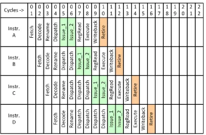
Figure 2.1 and figure 2.2 illustrate the above two scenarios. The x-axis is time, and
y-axis, instructions. The workload is a serially-dependent chain of instructions – i.e.,
instruction B depends on A, C depends on B, D depends on C etc. Figure 2.1
illustrates the running of this workload on a machine having the issue logic
sub-pipelined into two stages, Issue_1 and Issue_2. The data dependency between
adjacent instructions cause an instruction to issue only after its preceding instruction
Figure 2.1. Running a workload having serially-dependent chain of instructions on a machine with issue logic sub-pipelined into two stages. The propagation delay is not hidden by pipelining the issue logic.
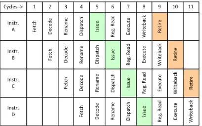
Figure 2.2 (scenario 2) has the same workload and machine, except that the pipeline
register that sub-pipelined the issue stage is removed – the machine has a
Figure 2.2. Running a workload having serially-dependent chain of instructions on a machine with unpipelined issue logic. Note that the x-axis represents time; the time period is twice that of figure 2.1.
Over a period of time, the pipelined and un-pipelined scenarios of figure 2.1 and
figure 2.2 have the same performance (neglecting pipeline latch delays and
pipelining imbalances). The argument here is that scenario 1 did not benefit from
pipelining (and higher clock frequency) due to the nature of the workload. If pipeline
latch delays and pipelining imbalances are also considered, scenario 2 (unpipelined)
would have a higher performance.
Instructions in the issue queue of a real workload are a complex mixture of
independent, ready instructions and dependent, not-ready instructions. Hence,
instructions enter the wakeup-select loop to overlap and hide the propagation delay.
The exact nature the impact on performance due to sub-pipelining the issue logic
can now be seen: If sub-pipelined too deeply, instructions will be unable to fill up the
wakeup-select loop and hide the propagation delay completely. If not sub-pipelined
deep enough, the processor is being underclocked for the amount of parallelism the
workload possesses.
2.2. Heterogeneity and Core Customization
Program behavior varies widely. Benchmarks used to represent real-world programs
differ in the amount of parallelism available and memory access patterns. This
variation is seen not just among benchmarks but even between phases within a
benchmark. Processor design is about finding the sweet-spot between various
trade-offs under given constraints, and the variation in program behavior forces the best
core design to the „average core‟ – the core that performs best on an average across
different program behaviors, or simply, across all benchmarks chosen to represent
real-life programs that the processor intends to run. The core is also designed to
ensure that the performance of a certain program behavior or a certain benchmark is
not degraded terribly – forcing the best design to be large and beefy, capable of
accommodating even program behaviors that demands lots of hardware resources
With Moore‟s Law adding transistors to the chip exponentially and a growing power
problem, processors have moved towards chip multicores to in search of
performance. The philosophy of designing cores has remained relatively the same –
the one-size-fits-all core is replicated on the chip to execute different threads or
programs in parallel. Heterogeneous multiprocessors (HMPs), i.e., designing cores
on a chip multicore differently and customizing each core to different program
behaviors, also called asymmetric cores in literature, is a promising concept for
extracting performance. The advantage of this organization is that each core is not a
compromise over the entire range of program behavior, but one over a certain
subset of it – with the sum total of all heterogeneous cores capable of handling all
program behavior reasonably well. Now that the range of program behavior each
core is expected to handle is smaller, less has to be compromised in the design of
each core, and therefore can achieve a higher performance for that program
behavior than the „average core‟. Each core is still an average core – but each core
is averaged over a smaller, different subset of all program behavior.
An open question in core customization is how different would the cores of a HMP
be from each other. In superscalar processors, hardware complexity is used to
extract IPC and pipelining is employed to mitigate the effect of the complexity on
frequency. Therefore, it is conceivable that the best core for most or all program
behaviors is a complex, very wide, large and deeply pipelined core – i.e., the beefy
best set of cores tends to be heterogeneous. The tighter the constraint the more
heterogeneous the cores become. Thus, area or power constraints act as forcing
functions for heterogeneity. The argument in this thesis is that depending on
program behaviors which expose the critical loops differently, propagation delay can
be a forcing function for heterogeneity – even if area and power budget is
unconstrained; and that the beefy core is not the best core for all program behavior.
The motivation for the argument that all workloads may not favor a single beefy core
is elaborated here: The inference from the analysis in section 2.1 is that the best
issue logic configuration is dependent very much on the nature of the workload –
how the dependent chains and independent instructions are distributed within the
workload. There are two scenarios in which the propagation delay of the
wakeup-select loop is exposed:
a) Lack of ready instructions in the issue queue, as described in section 2.1.3.
b) Processor flushing events such as exceptions, load-violations or branch
mispredictions (all of these are handled the same way in this thesis). The
processor waits until the offending instruction reaches the head of the Active
List (or Re-Order Buffer) and the entire processor is flushed. The flush clears
out all instructions in the wakeup-select loop, and exposes the propagation
delay, transiently till the loop is filled again.
i) Irrespective of how much the wakeup-select loop is pipelined, the
propagation delay is (almost) the same and hence, the impact of
exposing this critical loop is the same.
ii) The propagation delay is highest in the beefiest core, since this core is
very wide. Hence, the penalty of exposing the critical loop is highest in
the beefiest core.
The take-away from the above arguments is that the beefiest core (irrespective of
nature of sub-pipelining of the wakeup-select loop) need not have the best issue
logic for all workloads, especially if a) the workload lacks ILP or b) exceptions, load
violations and branch mispredictions are common enough so the propagation delay
(measured in seconds) is one of the major factors determining the performance
(inverse of the total time in seconds) of a workload.
2.3. FabIssue
Determining the best issue logic for a workload (section 2.1) is challenging, because
the dynamic window of instructions of workloads is a complex mixture of dependent
and independent instructions. It is difficult to characterize a workload by static code
information and predict its preferred issue logic configuration. Furthermore, flushes
of the processor are difficult to anticipate without actually running the workload. A
simpler approach is to simulate the workload on differently pipelined issue logic and
simulation of workloads in cycle-accurate simulators) but also clock frequency
estimate.
Studying propagation delay of the issue logic as a forcing function for heterogeneity
(section 2.2) is also challenging because it requires searching through a large
design space – designs that model propagation delay – to find the best designs for
different program behavior. If given the design space and a suitable design space
exploration technique, the designs of the cores customized to different program
behavior could then be used to construct a hypothetical heterogeneous core with
highest performance for the workload set, and calculate the (maximum possible)
performance benefit of heterogeneity.
What is required, thus, is a tool to generate issue logic designs based on input
parameters capable of providing timing information and IPC quickly. This was the
motivation to develop the FabIssue tool – a component of the FabScalar [2] toolset
that generates synthesizable RTL designs of issue logic of desired configuration –
as a part of this thesis. There are alternatives to this approach; they are discussed in
3. Related Work
3.1. Issue Logic
[15] studies the limits of extracting performance from ILP. An experiment in this limit
study varies the issue queue size (referred to in [15] as the continuously-managed
scheduler window size) and discovers that an issue queue size of 32 is sufficient to
extract ILP (i.e., get a high IPC) for the workloads considered. This thesis uses IPT
as a performance metric instead of IPC, and attempts to discover the best issue
logic configuration (issue width, issue depth and issue queue size) for different
workloads and phases within workloads.
[3] and [4] look at pipelining the issue logic without sacrificing atomicity of the
wakeup-select loop. But these techniques involve speculative instruction issue, and
incur a large penalty (in number of cycles) when speculation is incorrect. This thesis
does not deal with speculative instruction issue.
3.2. Design and Performance
The performance gain that can be obtained by matching core design to program
behavior has been explored in literature [16]. This thesis concentrates on the issue
logic and matches issue logic configuration to program behavior. The configuration
Kumar et.al [1] studies the benefit of heterogeneity in multicores when constraints on
area and power are applied and finds that the best set of cores are more
heterogeneous when area or power budget constraints are made tighter. This thesis
does not consider area or power budgets – instead asking the question, “Can
propagation delay of the issue logic itself cause the best set of cores to be
heterogeneous?”
3.3. Simulators
Cycle accurate processor simulators are perhaps, the computer architect‟s most
important window into the details of what exactly happens in a microprocessor.
There exists a spectrum of simulators from simple functional simulators [5] to ones
that model microarchitecture in detail [6], and depending on the details modeled, run
workloads to provide a wealth of runtime statistics, including IPC. These simulators
can also be easily made to model any processor configuration – it may be as simple
as changing a variable value in the simulator – and is valuable in studying
heterogeneity. They are usually written in C/C++ for speed and efficiency.
A drawback of C/C++ simulators is their inability to model timing – i.e., generate an
estimate of the clock frequency – as well as other technology-dependent parameters
like area and power. However, simulators can be used in conjunction with analytical
models [8], [9] that are capable of predicting technology-dependent parameters.
estimates from the analytical model. The accuracy of this approach is limited by the
level of detail of the analytical model. Even if the model is highly detailed, it is
debatable how well the model holds up once the technology changes. To be certain,
an analytical model would have to be recalibrated and re-validated for every
technology change.
An alternative to using cycle accurate simulators is to use RTL simulators. These are
written in a hardware description language like Verilog or VHDL, and by its very
nature, model microarchitectural features to a very file detail. A processor
configuration under study could be synthesized on any technology (all that is needed
is the technology library file) and an estimate of the clock frequency could be
obtained. The Illinois Verilog Model [11] is an attempt to create such a simulator.
However, it has been shown that the IVM is at times poorly synthesizable [12]. RTL
simulators also suffer from being slower in simulation time than a C/C++ simulator.
Furthermore, since the simulator is specified in RTL, it may be difficult to
re-configure the simulator to run another processor configuration – it may not be as
simple as changing a variable in the simulator. FabScalar [2] attempts to overcome
the above drawbacks and is described in detail in the following sub-section.
3.4. FabScalar
FabScalar enables automatic generation of synthesizable register-transfer-level
degree of sub-pipelining of pipeline stages. FabScalar views a superscalar
processor as a set of canonical pipeline stages that are stitched together to create
the processor. The flexibility to create arbitrary cores lies in the ability to configure
each pipeline stage in any way desired as long as the pipeline stage‟s interface and
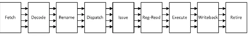
functionality is maintained. Figure 3.1 shows the canonical pipeline stages in
FabScalar.
Figure 3.1. Canonical Pipeline stages in FabScalar
Using FabScalar, answering the question, “What performance (IPT) does a workload
achieve on a core X” is answered very easily and quickly. The tool can be instructed
to generate the RTL of core X, which is synthesized to obtain an estimate of the
frequency. The workload can be run on a fast simulator – also part of the FabScalar
toolset – which is configured to match the generated RTL at cycle-by-cycle precision
to generate the IPC. Hence, workload the performance (IPT) on the core is obtained.
The RTL generated by FabScalar is intended to be synthesizable and provide a
reasonable estimate of clock frequency. A superscalar processor has many memory
structures, RAMs and CAMs that are not constructed out of logic gates or latches
(structures that Verilog can describe). Hence, included in the FabScalar toolset is
schematic, area, power and timing estimates of RAM and CAM structures. In order
to estimate clock frequency, the entire processor RTL generated by FabScalar
scripts (minus memory structures) is synthesized – the memory structures are
synthesized as black-box modules whose timing characteristics are got from
FabMem. Verilog descriptions of memory structures – RAMs and CAMs modeled
using flip-flops and logic gates – are also available in FabScalar in order to
functionally validate the RTL design by running workloads.
It is important to note that the frequency estimated by this approach – just like the
one obtained by an analytical model – may not absolutely match a fabricated
processor of the same configuration. This is because the layout generated by
synthesis and place-and-route tools does not involve the manually-done
pre-fabrication fine tuning that processors undergo, where designers tweak critical paths
by layout- and transistor-level alterations. However, automatic generation of
processor designs requires no design effort once the tool is in place. In the design
effort vs. accuracy trade-off seen here, FabScalar sacrifices some accuracy for zero
design effort. Even so, this approach using synthesis is still useful in understanding
how changing microarchitecture design affects IPC and frequency
4. Design of the Issue Logic
FabIssue, the set of scripts in FabScalar that deals with issue logic generation, has
an in-built issue logic design template. Depending on the input arguments to
FabIssue, it outputs the RTL of the desired issue logic design based on the
template. This chapter describes the template issue logic design.
4.1. Working of the Issue Logic
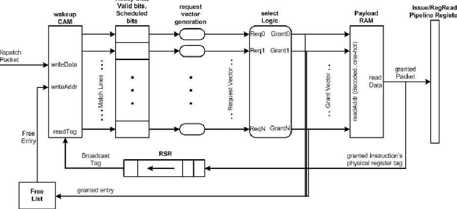
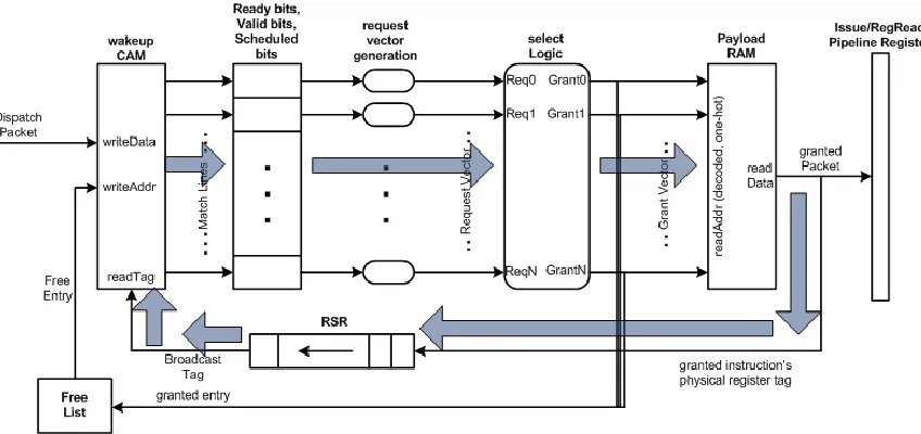
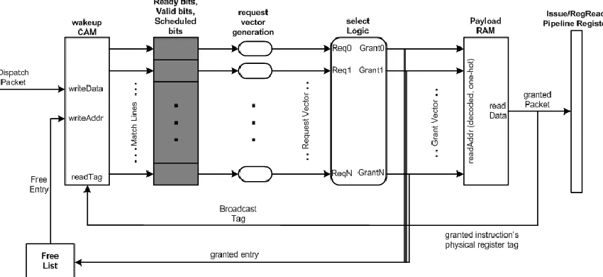
Figure 4.1 shows the components of the issue logic. The working of the issue logic is
broken down and described in the sub-sections below with respect to figure 4.1.
4.1.1. Dispatching an Instruction
When an instruction packet is dispatched from the front-end, the source physical
registers (and some control information) are stripped off from the packet and written
into the wakeup CAM. The rest of the packet is written into the payload RAM. The
reason for this division is that the entire instruction packet is not required for the
wakeup-select process – the source registers are sufficient. Hence the rest of the
packet placed in the payload RAM is read only when the instruction issues. The
number of entries in the wakeup CAM and the payload RAM are the same (called
issue queue size). An instruction is dispatched into the same entry location in the
CAM and RAM. This location, i.e., the issue queue entry at which the instruction is
dispatched into, is decided during the dispatch process by popping out a free
(unused) issue queue entry from the issue queue free list, a structure that maintains
a list of free entries in the issue queue.
4.1.2. Generation of Request Vectors
In addition to source physical register tags, an instruction also keeps certain control
bits (not in the CAM or RAM, but in flip-flops). These are:
a) Valid bit: A bit specifying if this issue queue entry is valid (being used).
b) Source valid bits: Two bits, one per source operand, specifying if the
instruction has a source operand. Instructions can have 0, 1 or 2 valid
c) Source ready bits: Two bits, one per source operand, specifying if the
source operand is available (or will be available when the instruction reaches
the function units for execution if issued now). These bits are initialized during
instruction dispatch by polling the physical register file valid bits. The source
ready bits are set in the wakeup process.
d) Scheduled bit: A bit specifying if this instruction has already been issued or
selected to be issued.
An issue queue entry that is valid, has all its valid source operands in the ready state
and has not been scheduled is said to be ready to issue. Ready instructions raise
the request line corresponding to its issue queue entry to let the select logic know
that it can issue now.
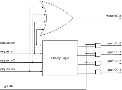
4.1.3. Select Logic
The select logic is priority logic that takes in all request vectors and generates a
one-hot grant vector. The grant vector lines feed the payload RAM read bit-lines, causing
the granted instruction‟s payload to be read out and sent down the pipeline. The
grant vector also sets the entry‟s scheduled bit.
Instead of monolithic priority logic block, the select tree is composed of smaller
select blocks, which when stitched together, functions like the monolithic priority
logic. With this approach, the select blocks can be manually designed and fine-tuned
composed using these select blocks. In this thesis, no fine tuning is done on the
select blocks, but the select logic is indeed constructed using select blocks (this
gives the flexibility of replacing select blocks generated by synthesis with manually
designed select blocks).
The select logic (also called select tree) is constructed using select blocks by
connecting them in a tree-like arrangement, with each successive level of the tree
having lesser select blocks than the previous, and the final level having one select
block. Figure 4.2 shows the logic in the 4:1 select block; this block has a 4-bit vector
input and a 4-bit, one hot vector output grantOut. grantOut signals function as the
grantIn signals to the select blocks that constitute the previous level of the select
tree. The select blocks also output requestOut, a signal that feeds a requestIn of the
select block in the next level of the select tree. The grant vector is the grantOut
Figure 4.2. 4:1 select block. grantIn comes from the next level of the select tree.
All select blocks (except the ones in the first level) choose between select blocks of
the previous level by sending grant signals to exactly one of them (if this select block
received grantIn from the next level). The first level select blocks uses the request
vector as input. It is thus, a hierarchical selection process.
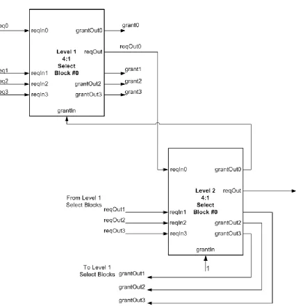
In Figure 4.3, part of a 16:1 select logic built out of 4:1 select blocks in a two level
fashion is shown. Request signals flow down the select tree (towards higher levels)
till the final stage of the select tree. grantOut signals flow up the select tree (towards
lower levels) to form the grant vector. The selection policy is static – a lower issue
Figure 4.3. Portion of a 16:1 select logic built out of 4:1 select blocks. req0 to req3 form the first 4 bits of the request vector and grant0 to grant3 are the first 4 bits of the final grant vector.
The select block at the final level of the select tree is given a grantIn signal that is
an instruction once every cycle, i.e., either the function units either have a latency of
one cycle or are fully pipelined.
4.1.4. Wakeup CAM
An issuing instruction broadcasts its destination physical register tag to all
instructions in the issue queue. Each instruction in the issue queue compares the
broadcasted tag to its source physical register tags, and on a match, sets the
corresponding source ready bit. This is the wakeup process. The comparison and
matching is handled by the wakeup CAM, which compares all its entries with the tag
placed at its read port (i.e., the wakeup port), and raises a set of match lines (which
feed the source ready bits). Since there are a maximum of two sources per
instruction, there are two wakeup CAMs, one per source register.
4.1.5. Result Shift Register
Instructions must be woken up as early as possible to maximize IPC. However, an
instruction woken up too early would reach the execute stage and finds that a source
register value is unavailable (not yet produced) and hence, cannot execute and
generate the correct result. Ideally, the instruction should be woken up so that if it
issues immediately after waking up, it finds that its source register value has just
been produced as it enters a function unit for execution. The value is then got via a
bypass from the outputs of the function units to the inputs of the function units.
and the value consumer instruction issuing must be, at least, the number of cycles
the producer instruction takes to execute.
The result shift register (RSR) enforces this minimum required delay between
issuing of the producer instruction and broadcast of its destination tag to wakeup
dependent instructions. When an instruction issues, it pushes its destination tag into
the tail of the RSR. The RSR shifts tags, once every cycle, towards its head, and
broadcasts the tag at its head to the CAM wakeup ports. Thus, the required delay
between issue and tag broadcast is got by fixing the number of registers in the RSR,
which is determined by the execution latency of the issuing instruction. If there are
instruction types differing in execution latencies, different RSRs are used for to each
instruction types.
4.1.6. Wakeup-Select Loop
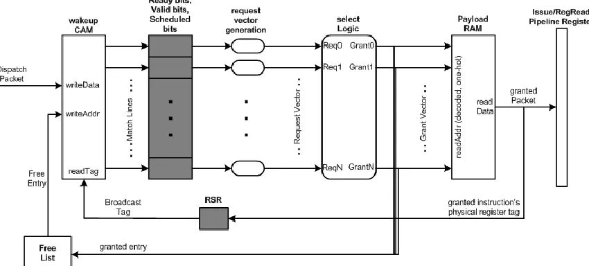
Figure 4.4 highlights the wakeup-select loop in the issue logic. The wakeup-select
loop starts at the ready bits of the instructions in the issue queue. The ready bits
contribute to the generation of the request vector, which feeds the select logic. The
grant vector generated by the select logic is used to read out the instruction‟s
payload from the payload RAM. One piece of information read from the payload
RAM, the instruction‟s destination physical register tag, is pushed into the RSR.
When the tag reaches the head of the RSR, it is fed into one of the read ports of the
wakeup CAM (a wakeup port). The CAM compares this tag with the source physical
lines set the ready bits of the corresponding source. This completes the loop from
ready bits to ready bits.
Figure 4.4. The issue logic shown with the wakeup-select loop highlighted
For best IPC, the wakeup process (setting of the ready bits) must be done so that
value consumer instructions are woken up „n‟ cycles after the value producer
instruction issues, where „n‟ is the execution latency of the producer instruction. This
way, the consumer instruction (if selected) will follow the producer instruction down
the pipeline at a distance „n‟ (measured in number of pipeline stages in between the
instructions, which is equivalent to number of cycles separating them). When the
consumer instruction reaches the function unit, its source value will have just been
For instructions with a single-cycle execution latency, consumer instructions have to
be woken up the very next cycle the instruction issues. This is possible only If the
wakeup-select loop is unpipelined, i.e., there are no pipeline registers in the
feedback path from ready bits to ready bits and the RSR latency is zero (that is,
RSR broadcasts tags the very cycle it receives the tags). For instructions with a
2-cycle execution latency, the RSR consists of a single register, so that tag broadcast
starts at the next cycle after issue, and wakeup happens two cycles after issue of the
instruction. An instruction with an n-cycle execution latency will use an RSR
consisting of (n-1) shift registers.
An exception to the above wakeup-select process is the load instruction.
Speculatively waking up load-dependent instructions (with no mechanism for
instruction replay in the issue logic) would be problematic if the load misses in the L1
cache: Dependent instructions reaching function units would find that its source
operand value is not available. Hence, loads have to be handled differently.
“Execution latency” of load instructions is unpredictable, and hence, when a load
issues, the exact number of cycles to wait before waking up its dependents is not
fixed. Therefore, loads do not broadcast destination register tags using the RSR.
Once a load executes and gets its value from the cache hierarchy, it broadcasts its
4.1.7. Free List Management
The free list keeps track of the used and free issue queue entries. When an
instruction is to be dispatched to the issue queue, a free issue queue entry number
is popped out from the free list and the instruction is written into that entry. When an
instruction is selected, the instruction‟s issue queue entry is written into the free list.
The actual freeing process (setting the issue queue entry‟s valid bit zero) may take
multiple cycles, and hence, in the interval between selecting an entry and resetting
its valid bit, the scheduled bit acts as the guard to prevent the entry from requesting
for selection again.
4.1.8. Cascaded Select trees
The backend of FabScalar processors have dedicated pipeline ways for different
instruction types. An instruction of a certain type can execute only in a pipeline way
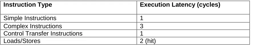
of its instruction type. The instruction types are given in Table 4.1.
Table 4.1. Instruction types in FabScalar and their execution latencies.
Instruction Type Execution Latency (cycles)
Simple Instructions 1
Complex Instructions 3
Control Transfer Instructions 1
Loads/Stores 2 (hit)
Four request vectors (one corresponding to each instruction type) are generated and
fed to four select trees. If the machine has an issue width of four (i.e., four pipeline
vector, which grants each selected instruction, access to one pipeline way (of its
type) to issue. But in a 5-wide issue machine (2 simple instruction pipeline ways, and
one pipeline way each for the other three types), the select logic processing
requests of simple instructions takes in a single request vector but outputs two
distinct one-hot grant vectors (one for each simple instruction pipeline way). Such a
select logic behaves like two cascaded select trees: the first works as a normal
select tree, while the second uses a masked-out request vector as its input, with the
request line corresponding to the entry selected by the first tree masked out. This
ensures that the two trees generate two distinct one-hot grant vectors. The idea is
extended to an n-cascaded select tree if there are n pipeline ways of an instruction
type.
Select trees can be placed in series to generate a cascaded select tree (the output
of a tree is used to mask the request vector it received, and then sent to the next
select tree‟s request vector input). This approach lets synthesis take care of the
complexity of designing the cascaded trees. Alternatively, select trees are
overlapped at the level of select blocks to create the cascaded select tree. Since
synthesis is done after flattening the RTL design, the two approaches are seen to
4.2. Pipelining the Issue Logic
Instructions with multiple-cycle execution latencies suffer no IPC degradation due to
pipelining the wakeup-select loop. This is because such instructions take multiple
cycles to wakeup consumers (reflected in the number of registers in the RSR used
by these instructions) and hence any extra delay (in cycles) in waking up consumers
due to sub-pipelining registers in the wakeup-select loop can be offset by reducing
the registers in the RSR correspondingly. For instance, a complex instruction with an
execution latency of 10 cycles uses an RSR consisting of 9 shift registers if the
wakeup-select loop is unpipelined, and an RSR consisting of 7 shift registers if the
wakeup-select loop is pipelined into 3 parts (two pipeline registers).
Hence, IPC degradation due to loss in atomicity of the wakeup-select loop affects
only instructions having an execution latency smaller than the loop depth (in cycles)
of the wakeup-select loop. But simple single-cycle instructions form a large portion of
integer workloads; hence IPC is markedly degraded for such workloads when the
loop is sub-pipelined.
The issue logic configurations described in this section here onwards are for
single-cycle execution latency instructions.
4.2.1. The 1/1 Issue Logic Configuration
The issue logic is unpipelined in the 1/1 issue logic configuration (figure 4.5). In this
when traversing the wakeup-select loop once; and the second “1” refers to the
number of pipeline registers encountered by an instruction during the entire issue
process. In terms of number of cycles, 1/1 means that consumer instructions are
woken up one cycle after the producer instruction issues, and that instructions spend
a minimum of one cycle in the issue stage. At least one pipeline register is
necessary in the wakeup-select loop, without which a combination feedback loop is
set up. Here, the ready bits act as a pipeline register between the CAM and the
select logic.
Figure 4.5. 1/1 issue logic configuration. Note that there is no RSR, since select and payload read and wakeup have to happen in the same cycle.
4.2.2. The 2/2 Issue Logic Configuration
The logical places to add pipeline registers to sub-pipeline the issue logic are
wakeup CAM. The 2/2 configuration (figure 4.6) adds a pipeline register between the
payload RAM and the wakeup CAM by adding a shift register to the RSR.
Figure 4.6. 2/2 issue logic configuration. Note that the RSR is a single register. The pipelining splits the issue logic into wakeup and select-payload read.
4.2.3. The 3/3 Issue Logic Configuration
This configuration adds a pipeline register in between the select logic and the
payload RAM. The grant vector produced by the select tree is used without passing
through the pipeline register to set the scheduled bits, and is used after passing
Figure 4.7. 3/3 issue logic configuration. Wakeup, select and payload read now happen in separate cycles for an instruction.
4.2.4. The 2/3 Issue Logic Configuration
The reason that the three configurations discussed above have the same
wakeup-select loop depth and issue stage depth is that the dependent instruction‟s wakeup
process needs the issuing instruction‟s destination physical register tag which is
stored in the payload RAM. Hence, an instruction‟s issue and the waking up of its
dependent instructions can both happen only after payload RAM read. However, if
the instruction‟s destination tag is available before the payload read, the wakeup
process can begin immediately after the selection process is completed. This can be
achieved by modifying the select logic to accept destination tags of instructions
along with the request vector, so that the tags can be multiplexed down the select
tree (in parallel with the selection process) and that the select tree produces the
destination physical register tags which feeds the select tree – written to when an
instruction is dispatched – is also required.
Figure 4.8. 2/3 issue logic configuration. The destination physical register tags are now got from the select tree instead of the payload RAM. The additional structure that holds the destination tags (and feeds the select tree) is written to during dispatch.
4.2.5 Pipelining the Select Logic
The select logic cannot be pipelined, because it would violate atomicity of the loop
that sets the scheduled bits (which prevent an already granted instruction from
requesting). That is, the loop starting at the scheduled bits, which contributes to the
generation of request vectors, feeding the select logic to produce the grant vector
used to set the scheduled bits – has to happen in one cycle. If not, an instruction
requested – leading to the possibility that an instruction is granted multiple times.
Hence, the select logic is not pipelined – this is seen to have important
5. FabIssue
FabIssue is the set of scripts in the FabScalar toolset that generates desired issue
logic designs. This section describes all scripts in FabScalar, and points out the
ones that are part of FabIssue.
Given the enormous complexity of generating arbitrary, functionally correct and
synthesizable cores, and the large number of parameters that can be varied in
superscalar cores, FabScalar divides processor attributes into two classes, which
are dealt with differently:
i) Sizes of structures within the processor
ii) Pipeline stage widths and sub-pipelining depths within pipeline stages
The first class, structure sizes, is handled within the RTL description by
parameterizing all structure sizes. Changing the value of the parameter that
describes the size of a structure (in the top level file where it is defined) is all that is
needed to create a different processor. Table 5.1 lists the attributes in the processor
which are parameterized.
Table 5.1. Parameterized processor attributes in FabScalar. The parameters that affect the issue logic are highlighted.
Branch Target Buffer Size Load Store Queue Size Branch Predictor Table Size Instruction Buffer Size
The second class of parameters is handled by scripts in FabScalar: Scripts (written
in Perl) that take in the widths and sub-pipelining depths of individual pipeline stages
as input and generates the RTL description (Verilog) of the processor. These scripts
function in a hierarchical manner: A single top-level script handles generation of the
entire processor and calls second-level scripts that handle generation of one pipeline
stage each; each second-level script calls third-level scripts to generate the Verilog
files in its pipeline stage. There is a 1:1 correspondence between third-level scripts
and Verilog files describing the processor, i.e., each third-level script generates one
Verilog file. Finally, third-level scripts may invoke module scripts, which generate
Verilog description of modules that have been instantiated within the Verilog file
generated by the third-level script. For example, IssueQSelect.pl, which generates
the select logic, calls SelectBlock.pl, which defines the select block module (the
select logic is composed of select blocks instantiations stitched together). The call
Table 5.2. Script call flow in FabScalar. The scripts that are part of FabIssue are highlighted
Top-Level Scripts Second-Level
Scripts Third-Level Scripts Module Scripts
Processor.pl fetch.pl FetchStage1.pl Fetch1Fetch2.pl FetchStage2.pl BranchPrediction.pl BTB.pl CTI.pl L1I.pl RAS.pl SelectInst.pl Fetch2Decode.pl SRAM_v.pl decode.pl Decode.pl PreDecode_PISA.pl Decode_PISA.pl InstBufRename.pl InstructionBuffer.pl RAM.pl rename.pl Rename.pl RenameMapTable.pl SpecFreeList.pl RenameDispatch.pl FREELIST_RAM.pl RMT_RAM.pl
dispatch.pl Dispatch.pl
issue.pl IssueQueue.pl freeList.pl cascadedIssueQSelect.pl IssueQSelect.pl issueqRegRead.pl CAM.pl cascadedSelectBlock.pl DecodedMux.pl Encoder.pl PriorityEncoder.pl PAYLOAD_RAM.pl RSR.pl selectBlock.pl
regread.pl regRead.pl
RegReadExecute.pl SRAM_PRF.pl
execute.pl AgenLsu.pl Execute.pl ForwardCheck.pl fu0.pl fu1.pl fu2.pl fu3.pl AGEN.pl Complex_ALU.pl Ctrl_ALU.pl Simple_ALU.pl
writeback.pl WriteBack.pl
retire.pl ActiveList.pl
ArchMapTable.pl AMT_RAM.pl
memory.pl LSU.pl L1DataCache.pl CommitLoad.pl CommitStore.pl DispatchedLoad.pl DispatchedStore.pl
fabscalar.pl FABSCALAR.pl
Interface.pl
6. Methodology
6.1. Experiments
The purpose of the experiments conducted in this thesis is to ascertain the
performance improvement from customizing issue logic to workloads. Hence, the
FabIssue tool is used to generate a range of cores which differ only in issue logic
configuration. All workloads are run on every generated core and performance (in
IPT) is tabulated. A hypothetical best multicore is constructed, consisting of the best
cores for each workload. The performance of the workload set on this hypothetical
heterogeneous multicore is compared with a homogeneous multicore consisting of
replicated copies of the single best core across all workloads (i.e., the average core).
The performance difference is the performance benefit of issue logic heterogeneity
quantified.
The above experiment is repeated at the granularity of phases within a benchmark.
The idea of core heterogeneity is to customize cores to program behavior, and not to
customize cores to benchmarks. Benchmarks typically have varying behavior in the
course of its run. This experiment generates IPT results for short segments within a
benchmark (short enough to be approximated to be a “phase” – i.e., a section of
code with unchanging program behavior). A full analysis of the relationship between
However, this experiment is intended to quantify the maximum performance gain
from customization to phase behavior, even if only issue logic is varied.
6.2. Assumptions and Limitations
This study tries to isolate the effect of varying issue queue configurations from the
rest of the processor. The metric used to evaluate a configuration is IPT. Hence, the
processor is configured to make IPC dependent on the issue logic as much as
possible (i.e., the issue logic is made the IPC bottleneck); and frequency is assumed
to be dictated by the issue logic.
To ensure that issue logic configuration is the IPC bottleneck, all other structures in
the processor are made large. The front-end width (fetch, decode, rename and
dispatch widths) is made very wide. Retire width is retained at four, but retire width is
confirmed to not be the bottle neck because (a) average IPC of any benchmark or
phase is never greater than four and (b) the active list is made large enough to
ensure that the active list never causes stalls due to a limited retire width.
There are certain restrictions and limitations in the current FabIssue tool with respect
to the mixture of function units that can be automatically generated:
a) The number of instruction types is fixed at four. Since each pipeline way in
the backend is dedicated to executing an instruction type, the minimum
b) The script infrastructure currently allows adding extra pipeline ways of the
simple instruction type only. A machine with a six-wide issue logic can only
have a backend configuration of (3,1,1,1), which stands for three simple
instruction pipeline ways, one complex instruction pipeline way, one control
instruction pipeline way and one memory instruction pipeline way. A five-wide
issue machine has the backend configuration (2,1,1,1). However, this is not a
very serious restriction – since the workloads run are integer benchmarks
where the majority of instructions are of the simple instruction type.
Caches are not modeled in the FabScalar toolset and hence, all load instructions are
hits. However, when a load issues, the processor does not assume a cache hit and
speculatively wake up load-dependent instructions – loads wakeup dependent
instructions only when it reaches the writeback stage.
6.3. Configuration of the Simulator
FabScalar processors follow the SimpleScalar [5] PISA and currently do not support
floating-point instructions. Hence, six SPECint2000 [10] benchmarks are used, and
the regions run are checked to not have any retiring floating-point instructions. All
simulations are 10 million instruction runs starting at SimPoints [7]. The input
Table 6.1. Benchmarks, input arguments and run starting points
Benchmark Input arguments Start of run (instructions)
bzip input.program 58 40.6 billion
Gap –q –m 64M 161.9 billion
Gzip input.graphic 60 77.4 billion
Mcf inp.in 44.1 billion
Parser 2.1.dict –batch 280.3 billion
Vortex lendian2.raw 40.8 billion
The simulator framework is set up to compare the PC, destination register tags and
destination register value of instructions retiring in Verilog with the SimpleScalar
functional simulator. Hence the functional correctness of the RTL design is validated
for each configuration for every run.
Issue width (and hence the processor backend configuration) is varied from 4 to 6
and 8. The issue logic sub-pipelining configurations used are 1/1, 2/2, 3/3 and 2/3.
The issue queue size is varied from 8 to 16 and 32. In total, 36 configurations are
created by all possible combinations of these parameters. The names given of the
configurations are of the format:
IS<issue_width>_<issue_depth_configuration>_<issue_queue_size>
For example, the largest and deepest pipelined configuration is IS8_3/3_32. The
Table 6.2. Configuration of the processor
Branch Target Buffer Size 4096 Fetch Width 8 Branch Predictor Table Size 65536 Fetch Depth 1 Return Address Stack Size 64 Decode Width 8
CTI Queue Size 32 Decode Depth 1
Instruction Buffer Size 64 Dispatch Width 8 Physical Register File Size 512 Dispatch Depth 1 Load Store Queue Size 32+32 RegRead Depth 1
Number of MSHR 8 Retire Width 4
Rename Map Table Size 34 Active List Size 512