46 A NUMERICAL SOLUTION OF TRAFFIC FLOW PROBLEM FOR ONE LANE
ROADWAY
Nurassikin binti Sahaian & Dr. Shazirawati binti Mohd Puzi
Abstract
This research is conducted to model flow of traffic on a one lane roadway by partial differential equation (PDE). Then, Finite Difference Method (FDM) is used to solve one-dimensional traffic flow equation. The Finite Difference Method involved is forward difference and central difference. In this problem, the density of cars with fixed ends is considered. The finite difference method (FDM) proceeds by replacing the derivatives in the traffic flow equations by finite difference approximations. This gives a large algebraic system of equations to be solved, which can be solved easily in mathematics software. MATLAB Distributed Computing R2010a software is used to perform the computational experiment while Microsoft Excel is used toillustrated the graphs. In this research, the effect of different step space, h and step time, k are investigated. Besides, comparison between finite difference solutions and analytical solutions will determine the accuracy of finite difference method (FDM).
Keywords: Traffic flow equation; Finite Difference Method; Macroscopic traffic flow model.
Introduction
Traffic flow is the interactions between drivers, vehicles, and infrastructure with the aim of developing an optimal road network with efficient movement of traffic and minimal traffic congestion problems. There are two classes of models in traffic flow problem which are macroscopic and microscopic. Macroscopic models concerned with average behaviour such as average speed, module area and traffic density while microscopic models concerned on individual behaviour. In this paper, the macroscopic models will be considered.
Method of characteristic is a technique for solving partial differential equations. This method is used to reduce a partial differential equation (PDE) to a family of ordinary differential equations (ODE).Meanwhile, finite difference method (FDM) is a numerical method for solving differential equations by approximating them with difference equations, in which finite differences approximate the derivatives. However, when FDM isused to treat numerically a PDE, the differentiable solution is approximated by somegrid function.
This research is aimed to model flow of traffic on a one lane roadway by partial different equation and solved by characteristic method and finite difference method. Purpose for modeling this model is to estimate number of cars on a one lane roadway and minimal congestion of traffic problem.Besides, we have to determine the accuracy of finite difference method.
47 the density is continuous, ignored the behaviour of individual driver and each car has the same size.
Literature Review
In 1930’s, the scientific study of traffic flow had begun by Greenshields (1935) with the study of models relating volume and speed with the pioneer in the use of photography relating to traffic matters and applying mathematics to traffic flow. Then, continued with the application of probability theory to the description of road traffic by Adams (1936) and the investigation of traffic performance at urban street intersections (Greenshieldset al., 1949) In 1950’s, theoretical developments based on a variety of approaches, such as car-following, traffic wave theory which is hydrodynamic analogy and queuing theory by Wardrop (1952), Pipes (1953), Lighthill and Whitham (1955), Newell (1955), Edie and Foote (1958), and Chandler et al. (1958).
Traffic flow model has been modified to various models and they are solved by differential equation or partial differential equation. For example, Alkhazraji (2008) focused on modification of non-linear car following model and generally aimed at improving the validity of the model; Sohrweideet al. (2001) compared between four-lane arterial roadways and three-lane roadway with a centre two way left-turn lane in their work to identify which lane provided the traffic calming; Cocliteet al. (2005) concerned with a fluid dynamic model of heavy traffic flow on a road. Precisely, they consider single conservation law, defined a road network with junctions and concluded from conservation of number of cars;Doboszczak and Forstall (2013) modelled the flow of traffic on a one lane roadway by partial differential equation (PDE) with assuming the velocity is constant for all cars, density is continuous and ignoring the individual behavior and other effects such as weather, accident and construction; Sultana et al. (2003) considered a fluid dynamic traffic flow model appended with a closure linear velocity-density relationship which provides a first order partial differential equation (PDE). Besides that, initial boundary value problem is treated in the paper. Analytical solution of traffic flow is present as Cauchy problem while a numerical solution of traffic flow model with initial boundary value problem is performed based on a finite difference scheme.
Traffic density and car velocity are related by only one equation, conservation of car
Herman (1977) assumed that under all circumstances the driver’s velocity is a known function of , determined by
Then, (Alkhazraji, 2008) stated that the partial differential equation which was formulated to mathematically model traffic flow is
( )
48 This research is aimed to model flow of traffic on a one lane roadway by partial different equation. The traffic flow model is solved explicitly by characteristic method and finite difference. At the end of the research, we will find out the models flow of traffic on a one lane roadway. With this model, it will show us how to approximate the number of cars in specific distance and reduce congestion traffic flow with some conditions.
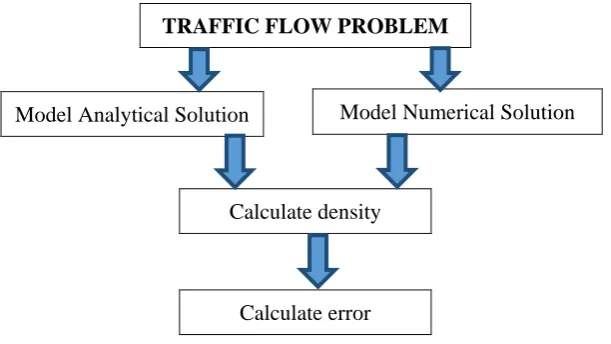
TRAFFIC FLOW PROBLEM
Figure 1: Procedure flow of finding accuracy of finite difference method.
Analytical Solution 0f Traffic Flow Model
Sultana et al. (2003) assume all cars have some constant velocity Then, from the relationship among density, flux and velocity, the flux yields the equation of the continuity
in the form
In this case, consider velocity
as a function of density (Ailkhazraji, 2008). Then, substitute equation (3) into equation (2), equation become
Equation (4) is a first order partial differential equation and nonlinear in This yield
After that,
( )
which is linear in derivatives but non-linear in , termed as quasi-linear equation.
( (
) ) Kabiret al. (2010) use a non-linear speed density relation which is in the form as equation (6). Then, a non-linear speed density relation will give relationship for the traffic flux
Model Analytical Solution Model Numerical Solution
Calculate density
49 (
) Then, if equation (3.10) is put into the general non-linear model partial differential equation (3.8), the explicit non-linear partial differential equation is obtained as in the form
( ( )) with . Initial value problem (8), can be solved by the method of characteristics. The partial differential equation in the initial value problem (8) can be written as
where
(
)
and its derivative is
(
)
Therefore,
implies
(
) Thus,
after applying the characteristic method on the partial differential equation.Hence,
(
) Integrating equation (9) yields
∫ ∫
∫
When equation (10) is integrated both sides, we get
∫ ∫ ( ) and yields
(
) Next, equation (12) gives
(
) which are the characteristics of the initial value problem (8). From equation (11), it turns to
since the characteristics through also passes through and is constant on this curve, thus initial condition is used to write
50 Equation (14) and (15) yield
while equation (13) gives
( ) Therefore, substitute it into equation (16) gives the form
( (
) ) Thus, this is the analytical solution of characteristic method for the problem (1).
Numerical Solution of Traffic Flow Model
A finite difference scheme for traffic model problem is:
with initial condition
and boundary conditions
where
( (
) )
From Taylor’s series, apply forward difference formula in time and write
and thus,
( )
Then, apply central difference formula in space. From Taylor’s series, write
51
and thus,
( )
Assume
( )
and the uniform grid spacing with step size h and k for space and time respectively:
and
Next, substitute (20) and (21) in (18), the discrete version of the non-linear partial difference equation formulates the first order finite difference scheme of the form
( ) where
The difference equation is known as Lax-Friedrichs scheme where
( (
) )
Thus, this is the numerical solution of the first order finite difference scheme for the problem (18).
Absolute error =
Relative error =
Mean square error = ∑ 2
Results and Discussion
We let
with initial condition
and boundary condition
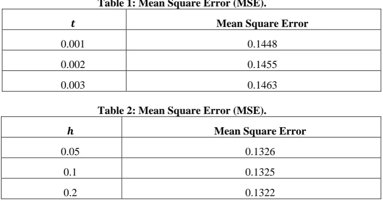
52 Table 1: Mean Square Error (MSE).
Mean Square Error
0.001 0.1448
0.002 0.1455
0.003 0.1463
Table 2: Mean Square Error (MSE).
Mean Square Error
0.05 0.1326
0.1 0.1325
0.2 0.1322
Based on the experiment that have been carried out, it can be summarized that the different values of step time, and step space, different value of absolute error, relative error and mean square error. From the results, it give that as the value of is increased, the mean square error also increase. Therefore, it can be concluded the different values of step time, k give the best approximations when the step time, is smaller
Besides that, the smaller value of step space, does not gives good approximation to the analytical values because the mean square error is decreasing due to the increasing value of step space, . From all finding we obtained, it shown that finite difference method gives better approximation to the analytical solution when the step space, is smaller.However, the error obtained is big. This solution may not as good as other method to get better accuracy for this problem. As a summary, finite difference method is a good method which is capable to solve the one-dimensional traffic flow equation but for this problem, however it may not adequate enough.
Conclusion
This research is aimed to study on the finite difference method for traffic flow equation. The effect of different step time, and step space, has been discussed in this study. In addition, the accuracy of finite difference method is determined by calculating the absolute error, relative error, and mean square error. Later on, the results will be compared with the analytical solution of the traffic flow problem. Moreover, the approximation solution of finite difference method also has been calculated by using MATLAB Distributed Computing R2010a software.
53 References
Alkhazraji, A. S. A., (2008). Traffic Flow Problem with Differential Equation. AL-Fatih Journal. No.35.
Adams (1936). Road Traffic Considered as a Random Series. Journal of the Institute of Civil Engineers. London. 4, 121-130.
Braun, M., Coleman, C. S., and Drew, D. A. (2012).Differential Equation Models. New Jersey, U.S.A.: Springer.
Bressan, A. (2000). Hyperbolic Systems of Conservations Laws The One Dimensional Cauchy Problem. Oxford Uni. Press. Oxford.
Coclite, G. M., Garavello, M., and Piccoli, B. (2005).Traffic Flow on a Road Network.SIAM J. Math.Anal. 36(6), 1862-1886.
Chandler, F. E., Herman, R., and Montroll, E. W. (1958). Traffic dynamic: Studies in Car Following. Operation Research. 6(2), 165-184.
Che Rahim CheTeh (2013). Numerical Method: AigorithmAndMatlab Programming. (pp. 209-243). UniversitiTeknologi Malaysia: Esktop Publisher.
Daganzo, C. F. (Ed.) (1993). Transportation and Traffic Theory. Berkeley: Elsevier.
Doboszczak, S., and Forstall, V. (2013).Mathematical Modeling by Differential Equations.In Holmes, M. H. Introduction to the Foundations of Applied Mathematics. (pp. 205-254). United States: Springer
Edie, L. C., and Foote, R. S. (1958). Traffic Flow In Tunnels. Highway Research Board Proceedings.6-10 January. Washington, D.C., 334-344.
Greenshields, B.D. (1935) A Study of Traffic Capacity.Proceeding Highway Research Record.Washington, 448-477.
Greenshields, B.D., Schapiro, D., and Erickson, E. L. (1949) Traffic Performance at Urban street Intersections.Journal of the American Statistical Association.West Street, New York, 142-144.
Herman, R. (Ed.) (1961). Theory of Traffic Flow. Amsterdam: Elsevier.
Holmes, M. H. (2009). Introduction to the Foundations of Applied Mathematics. (pp. 205-254). United States: Springer.
Kabir, M. H., Gani, M. O. and Andallah, L. S. (2010).Numerical Simulation of a Mathematical Traffic Flow Model Based on a Nonlinear Velocity-Density Function.Journal of Bangladesh Academy of Sciences.34(1), 15-22.
Lee, K., Feron, E., and Pritchett, A. (2006).Air Traffic Complexity.Proceeding of the 44th Annual Allerton Conference.Illnois, 1354-1363.
Lighthill, M. J., and Whitham, G. B. (1955). On Kinetic Waves I: Flood Movement in Long Rivers. II. A Theory of Traffic Flow on Long Crowded Roads.Proceedings of Royal Society. 17 March. London, 281-345.
Machomikemd (2014).Retrived on June 28, 2014, from http://www.virtualtourist.com/. Newell, G. F. (1955). Mathematical Models for Freely Flowing Highway Traffic.Journal of the Operational Research Society of America. 3(2), 176-186.
Pipe, L. A. (1953).An Operational Analysis of Traffic Dynamic.Journal of Applied Physics. 24, 271-281.
Sultana, N., Parvin,.M., Sarker, R., and Andallah, A. (2013). Simulation of Traffic Flow Model with Traffic Controller Boundary.International Journal of Science and Engineering.
5(1), 6-11.
Sohrweide, P. E. T. A., Buck, B. P. T. O. E, Wronski, P. E. R. (2001). Arterial Street Traffic Calming with Three-Lane Roads.
Wardrop, J. G. (1952). Some theoretical Aspect of Road Traffic Research. Proceeding of