Article
1
Chilled station optimization operation based on
2
TRNSYS simulation of an existing public building
3
Baogang Zhang 1, Chang Sun 1, Ming Liu 2,* and Lin Lv 1
4
1 Department of Construction Engineering, Dalian University of Technology, Dalian 116024, China;
5
[email protected](B.Z.); [email protected](C.S.); [email protected](L.L.)
6
2 School of Architecture, Dalian University of Technology, Dalian 116024, China; [email protected]
7
* Correspondence: [email protected]; Tel.: +86-187-4551-7337
8
9
Abstract: Taking an existing public building as an example, on the basis of the measured data, the
10
mathematical model of each equipment module of the chilled station and the TRNSYS custom
11
module are established. The mathematical model of “chilled station cooling capacity—equipment
12
power” is proposed and established. The full-frequency control strategy based on device
13
contribution rate is proposed and established to set up the Matlab control module of the chilled
14
station. The TRNSYS simulation platform is used to simulate a public building chilled station in
15
cooling season. The result shows that the season energy efficiency rate of the public building
16
air-conditioning system is 2.15 times the original after applying the new control strategy.
17
Keywords: chilled station, TRNSYS, control strategy, operational energy efficiency
18
19
1. Introduction
20
32 domestic public buildings are researched only to find that the current air-conditioning
21
system's chilled station equipment is mostly controlled by artificially changing the number of
22
operating devices. The air-conditioning terminal is not adjusted and the automatic control system is
23
in a paralyzed state actually.A small number of public buildings using automatic control systems
24
still have the problem of low energy efficiency in air-conditioning projects.
25
Some scholars have conducted research on this, and research shows that the energy saving of a
26
single device does not mean that the system is energy-efficient. The full conversion of the chilled
27
station can significantly increase the energy efficiency of the system[1-5]. The Hopfield neural network
28
(HNN) can be used to predict the chilled water supply temperature[6-8], simulated annealing
29
algorithm, BP algorithm, and Sub-models and other optimization algorithms can solve the
30
optimization problem of multidimensional nonlinear constrained central air conditioning systems,
31
and thus obtain the set values of the most supervised control strategy control variable[9-16]. TRNSYS
32
simulation platform can be used to calibrate experimental data and energy simulation of
33
air-conditioning systems, and optimize control Strategy[17-22].
34
This article takes one of the public buildings used the automatic control system as the research
35
object for analysis and calculation and the air conditioning system's terminal regulation is not
36
considered. The optimal control strategy for the chilled station is studied in this article.
37
2. Research object
38
2.1. Basic information
39
This article examines an existing public building (hereinafter referred to as test building) in
40
Dalian. The nameplate parameters of the air-conditioning system's equipment are shown in Table 1.
41
It is equipped with an air-conditioning automatic control system, a direct digital control system
42
(DDC system), and chilled water. A flow bypass valve is provided between the inlet and outlet
43
pipes, and the water supply amount is changed according to the set supply and return water
44
temperature difference so as to adapt to changes in the system load. The cold season is from July 1
45
to September 30, a total of 92 days, and the operation time is 8:30 to 17:30 with the daily operation
46
of 9 hours.
47
Table 1. The nameplate parameters of each equipment of the air condition system
48
Device name Nameplate parameter
Chiller Q=1383.2kW;N=265.7kW
Cooling water pump G=319m3/h;H=27m;r=1450r/min;N=37kW
Cooling tower G=320m3/h;cooling water37/32℃;N=5.5kW*2
Chilled water pump G=262m3/h;H=33m;r=1450r/min;N=37kW
Fan coil Total 280.32kW
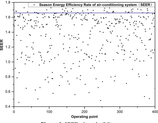
VRV Total 435.25kW
400 sets of operation data for the summer of 2017 were selected in order to analyze and
49
calculate the operating characteristics of the building chilled station.
50
2.2. Operating characteristics
51
The operating characteristics of the air-conditioning system include the energy efficiency of a
52
single device and the energy efficiency of the system. This article uses the chiller energy efficiency
53
rating and the Season Energy Efficiency Rate in air-conditioning system(SEER) as the operating
54
characteristic parameters. In order to test whether the SEER meets the design requirements, the
55
air-conditioning engineering design energy efficiency ratio is introduced.
56
2.2.1. Chiller energy efficiency rating
57
The energy efficiency rate of chillers[23] is determined based on the coefficient of performance
58
and the overall partial load performance coefficient, which are in turn divided into three levels of 1,
59
2, and 3, with the first level representing the highest energy efficiency. “Energy efficiency limit
60
values and energy efficiency grades for chillers” (Chinese standard GB19577-2015) stipulates that
61
the test value and labeling value of coefficient of performance (COP) and IPLV of water-cooled
62
chillers should not be less than specified value corresponding to the energy efficiency class in Table
63
2.
64
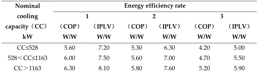
Table.2. Water-cooled chiller energy efficiency rating
65
Nominal
cooling
capacity(CC)
kW
Energy efficiency rate
1 2 3
(COP)
W/W
(IPLV)
W/W
(COP)
W/W
(IPLV)
W/W
(COP)
W/W
(IPLV)
W/W
CC≤528 5.60 7.20 5.30 6.30 4.20 5.00
528<CC≤1163 6.00 7.50 5.60 7.00 4.70 5.50
CC>1163 6.30 8.10 5.80 7.60 5.20 5.90
The nameplate calibration COP of the chiller unit is 5.20. The actual COP of the chiller at
66
68
Figure 1. Chiller COP at different host load rates
69
On the whole, the chiller COP increases with the increase of the host load rate, but there is
70
no obvious relationship between the changes, and the operation energy efficiency of the
71
chiller is not stable.
72
The average COP of the chiller is 4.44, with a maximum value of 5.00, which does not reach
73
the nameplate calibration value.
74
The host runs 32.25% of the time below 50% load.
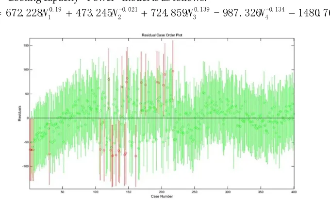
75
2.2.2. Design energy efficiency rate of air conditioning engineering(DEER)
76
The formula for DEER[24] is as follows:
77
N Q
DEER (1)
78
where ∑Q is the design cooling load for air conditioning(kW), ∑N is the total power consumption of air
79
conditioning(kW).
80
"Limit of DEER" refers to the average of the design energy efficiency ratio of air-conditioning
81
engineering for various types of cold source, and is the bottom line of the air-conditioning engineering design
82
energy efficiency ratio. At present, there is no study on the DEER limits of office buildings in Dalian, but
83
some scholars have studied the DEER limits of office buildings in Chongqing, as shown in Table 3.
84
Table.3. The DEER limits of office buildings in Chongqing
85
Cold source
Air-cooled
heat pump
chiller
Screw
chiller
Centrif
ugal
chiller
Variable frequency
VRV air
conditioning system
LiBr
absorption
chiller
DEER limits 2.40 2.89 3.25 2.20 2.60
Chongqing has high daytime temperatures in summer, the nighttime temperatures are hot and
86
the outdoor environment is less comfortable. Research shows that DEER limits are higher in areas
87
with higher outdoor comfort[24]. During the day in Dalian, the land temperature is high and the
88
ocean is blowing wind from the sea to land; the nighttime wind blows from the land to the sea, and
89
the comfort of the outdoor environment is higher. Therefore, the DEER limit in Dalian is higher
90
than that in Chongqing.
91
The design cooling load of test building is 2350kW, so its DEER is equal to 1.66 according to
92
formula (1) and Table 1, which is obviously does not meet the requirements of DEER limits for
93
office buildings in Dalian.
94
2.2.3. Seasonal energy efficiency rate of air conditioning engineering(SEER)
96
The formula for SEER[24] is as follows:
97
N Q
SEER n
(2)
98
where Qn is the cold load at different partial load rates(kW), N is the total power consumption of
99
air-conditioning works under partial load(kW).
100
The SEER is shown in Fig.2. after calculating.
101
102
Figure 2. SEER of test building
103
The average SEER of the test buildings is 1.34, and it does not reach the design energy
104
efficiency ratio at 90.25% of the operating conditions.
105
From the above analysis, it can be seen that the chiller has unstable operation energy efficiency,
106
the DEER is lower than the limit value, and SEER cannot reach the design energy efficiency ratio. In
107
the following, the mathematics model of equipment is established and the optimization strategy is
108
proposed for the problems existing in existing public buildings. Simulations are performed using
109
the TRNSYS simulation platform.
110
3. Mathematical models of chilled station equipment
111
According to the measured data, parameters of the equipment model can be identified.
112
Parameter identification determines a set of parameter values based on the experimental data and
113
the established model, so that the numerical results calculated by the model can best fit the test data
114
so that the unknown process can be predicted. When the predicted results match the measured
115
results, this model can be considered to have high credibility. The parameter identification of the
116
model requires the least square estimation of the model parameters. The basic idea is as follows.
117
Find an estimate of θ defined as θ so that the sum of the squares of the difference between
118
the actual measurement Zi (i=1,..., M) and the measurement estimate which is Z = H θ determined
119
by the estimate is minimized.
120
3.1. Mathematical model of single equipment
121
Some scholars have studied the MP model of the chilled station equipment[25]. In this paper, the
122
parameters of the equipment model are identified based on the measured data. The selected 400
123
sets of data are preprocessed, 250 sets of data are used to identify the parameters of the equipment
124
model using Origin software, and 150 sets of data are used to test the accuracy of the model.
125
Taking the chiller as an example, the selected 250 sets of measured data are input into Origin to
126
identify the parameters of the chiller model. After many iterations, the parameter estimation
127
reaches the convergence criterion, and the obtained parameter value retains three significant digits
128
477
,
1
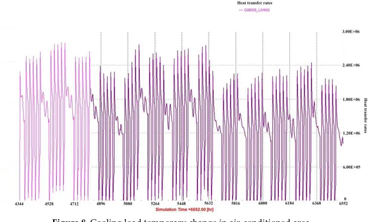
.
30
-,
856
.
0
,
00614
.
0
B
C
D
A
130
So the chiller model obtained is:
131
477 1 . 30 -856 . 0 00614 . 0- 2 1
1 3
1
1 k k k
N (3)
132
where N1 is the chiller actual power(kW), k1 is the chiller motor operating frequency(Hz).
133
134
Figure 3. Chiller model fitting results graph
135
In order to further verify the accuracy of the model, the remaining 150 groups of measured
136
data are used to predict and verify the chiller model that has completed parameter identification.
137
138
Figure 4. Chiller model fitting residual map
139
As can be seen from the figure,the relative error between the measured value and the
140
predicted value can be kept within 5% in 150 sets of data. The error variance of the identified model
141
is 0, and the correlation coefficient is 1, indicating that the identified model can accurately predict
142
the measured data. Therefore, the identification model can be used in the subsequent study.
143
After the simulation and test, the residual values of the predicted values and actual values of
144
other equipment models are all within 5%, and each equipment model is as follows.
145
2 2 2
2
0
.
00138
k
0
.
00289
G
k
H
(4)146
552 . 0 247 . 0 0663 .0 -1 2
2 2 2 2 -2
2 k G k G
(5)
147
0
.
55
81
.
3
0874
.
0
10
46
.
4
-
2 22 3
2 4
2
k
k
k
N
(6)148
2 3 3 3 2 33
0
.
00819
k
0
.
00173
k
G
-
0
.
000168
G
H
(7)149
520 . 0 00192 . 0 0561 . 0- 1 3 3
3
3 kG G
(8)
150
8
.
11
-439
.
0
0124
.
0
10
10
.
6
2 33 3
3 5
3
k
k
k
N
(9)
151
3 4 5 3 ct 44 N 8.8 10 k
k k
N ct
(10)
152
where H2 is the chilled water pump head(m), G2 is the chilled water pump flow(m3/h), k2 is the
153
motor operating frequency of chilled water pump(Hz), η2 is the chilled water pump efficiency(%), N2 is
154
the chiller water pump actual power(kW), H3 is the cooling water pump head(m), G3 is the cooling
155
water pump flow(m3/h), k3 is the motor operating frequency of cooling water pump(Hz), η2 is the
cooling water pump efficiency(%), N3 is the cooling water pump actual power(kW), N4 is the cooling tower
157
actual power(kW), k4 is the motor operating frequency of cooling tower(Hz), kct is the motor rated
158
frequency of cooling tower which is equal to 50(Hz).
159
3.2. Mathematical model between chilled station output cooling capacity and equipment power
160
This article proposes and establishes the "output cooling capacity - equipment power"
161
(hereinafter referred to as "Cooling capacity - Power") model of the chilled station. It is assumed
162
that the MP model is as follows.
163
I GN EN CN ANQ B D F H
1 2 3 4 (11)
164
where Q is the output cooling capacity(kW), N1 is the chiller actual power(kW), N2 is the chiller water
165
pump actual power(kW), N3 is the cooling water pump actual power(kW), N4 is the cooling tower actual
166
power(kW), A/B/C/D/E/F/G/H/I is the model identification parameters.
167
Using the 400 sets of measured data to identify the parameters of the "Cooling capacity-Power"
168
model, the results are as follows.
169
859
.
724
,
.021
0
-,
245
.
473
,
190
.
0
,
228
.
672
B
C
D
E
A
170
762 . 1480 -, 134 . 0 -, 87.326 9 -, 139 .0
G H I
F
171
Thus the “Cooling capacity - Power” model is as follows.
172
762
.
1480
87.326
9
-859
.
724
245
.
473
228
.
672
-0.1344 139 . 0 3 .021 0 -2 19 . 0
1
N
N
N
N
Q
(12)173
174
Figure 5. “Cooling capacity - Power” model fitting residual map
175
3.3. Chilled station optimization control strategy
176
At present, the air-conditioning engineering automatic control system is mostly PID control
177
mode which structure is simple and stable. The PID control of the primary pump variable flow
178
system makes the chilled station have a certain self-adaptive capacity for changes in the building
179
load, but the central air conditioning system is nonlinear and has strong hysteresis. The system is in
180
low control effectiveness when the building load changes greatly. A optimized control strategy is
181
established based on the device contribution rate according to the “Cooling capacity - Power”
182
model.
183
The device contribution rate is the ratio of the amount of change in cooling capacity to the
184
amount of power change in a device when the cooling capacity changes. Taking a single chiller as
185
capacity reduces from 500kW to 480kW, the power of the chiller reduces from 300kW to 290kW.
187
The contribution of the chiller is
2 10 20 290 -300 480 -500 .
188
Matlab is used to find the minimum power value of each device at a given cooling capacity.
189
The samples of the chilled station equipment are checked to obtain the input power variation
190
range of each equipment. Simulation is done in the TRNSYS platform using the cold load module
191
and the chilled station equipment module to output the temperature of the chilled water in and out
192
of the chiller, the cooling capacity, the input power of each equipment, and obtain the temperature
193
difference variation range of chilled water in and out of the chiller.
194
FunctionG is set in which the chilled water pump power, frequency, and flow are input. When
195
using, N2 is input and k2 can be calculated according to equation(6), then functionG is called out to
196
output the value of chilled water pump flow G2.
197
Cooling capacity is represented by Qcc, chiller power N1, chilled water pump power N2,
198
cooling water pump power N3, cooling tower power N4, and the temperature difference of chilled
199
water in and out the chiller is △t. Objective functionminN min
N1 N2 N3 N4
.200
The constraints are as follows.
201
42 . 8 52 . 2 32 . 25 68 . 14 01 . 24 56 . 12 98 . 217 16 . 119 46 . 5 12 . 3 8 . 58 66 . 4 122 . 0 10 32 . 8 4 3 2 1 2 2 2 3 2 4 2 2 cc N N N N t k k k N t G c Q 202
Under the condition of one chiller to one water pump to one cooling tower and no control
203
module, the cooling capacity of the chilled station reduces from 1220kW to 1200kW. The cooling
204
capacity and power of each device are shown in the table below.
205
Table.4. The cooling capacity and equipment power change of chilled station
206
Cooling capacity(kW)
Actual input power of chilled station equipment(kW)
Chiller Chilled water pump
Cooling water
pump Cooling tower
1220 213.39 19.28 24.60 6.60
1200 209.52 18.97 24.50 5.96
Device contribution rate 5.17 65.13 190.56 31.37
It can be seen that when the cooling capacity is 1200 kW, the ratio of the cooling capacity to the
207
total input power of the chilled station equipment (chilled station COP) is 4.63. The chiller has the
208
lowest contribution rate, and the cooling water pump equipment has the highest contribution rate.
209
Therefore, increase the input power of the chiller and reduce the input power of the cooling water
210
pump to find the minimum total input power with cooling capacity of 1200kW.
211
Matlab is used to find the optimal value and the result is shown in table. 5. When the input
212
power of the device is as follows, the cooling capacity is guaranteed to be 1200 kW and the total
213
input power of the device is the minimum.
214
Table.5. The minimum input power of chilled station equipment under the same cooling capacity of 1200kW
215
Device Chiller Chilled water pump Cooling water pump Cooling tower
Input power(kW) 211.52 17.41 22.73 4.73
Device contribution rate 10.70 10.71 10.69 10.71
The chilled station COP is 4.74 after optimization, which is 1.00% higher than before. It can be
216
whether the optimal value of device contribution rate is always the same or not under different
218
cooling capacity, cooling capacity from 1220kW to 1180 kW, 1160kW and 1140kW are verified and
219
the results are as follows.
220
Table.6. Device contribution rate under different cooling capacity
221
Cooling capacity(kW)
Actual input power of chilled station equipment(kW)
Chilled station COP Chiller Chilled water pump Cooling water pump Cooling tower Total power
1180 before fixing 207.24 18.87 24.48 5.90
256.49 4.60 Device contribution rate 6.50 98.36 330.49 57.34
1180 after fixing 210.41 16.30 21.62 3.62
251.95 4.68 Device contribution rate 13.42 13.44 13.42 13.43
1160 before fixing 206.96 18.66 23.97 5.98
252.58 4.59 Device contribution rate 9.33 97.30 95.08 194.29
1160 after fixing 209.96 15.86 21.19 3.18
250.19 4.64 Device contribution rate 17.49 17.56 17.59 17.56
1140 before fixing 205.59 18.32 23.92 5.09
252.58 4.51 Device contribution rate 2.44 144.93 90.84 106.75
1140 after fixing 209.59 15.48 20.61 2.81
248.49 4.59 Device contribution rate 21.05 21.07 20.04 21.12
It can be seen that the optimal value of device contribution rate is the same and the chilled
222
station COP increases by 1.80%, 0.96%, and 1.65% with the cooling capacity 1180kW, 1160kW, and
223
1140kW at this condition. Thus it can be concluded that the chilled station COP is the highest when
224
the freezing plant device contribution rate is the same in the case of a certain amount of cooling
225
capacity, and the optimal control strategy is established base on this.
226
Taking the seasonal energy efficiency ratio (SEER) as the objective function, a new chilled
227
station control strategy based on the device contribution rate is established combined with the
228
“Cooling capacity-Power”model.
229
According to the known "Cooling capacity-Power" model, the device contribution rate of each
230
equipment is as follows.
231
Table.7. Device contribution rate of chilled station equipment
232
Device Device contribution rate
Chiller 1
1 805 . 52 N N Q
Chilled water pump 2
2 640 . 839 N N Q
Cooling water pump 3
3 628 . 20 N N Q
Cooling tower 4
4 607 . 47 N N Q
The device contribution rate is the same which is 1 2 3 N4
Q N Q N Q N Q
, so that
233
4 3
2
1 839.640 20.628 47.607 805
.
52
N
N
N
N
(13)234
The cooling load changes when the outdoor weather conditions change, so that the cooling
236
capacity is known.
237
In conjunction with function (12) and (13), the input power of chilled station equipment can be
238
obtained.
239
According to the "power-frequency" model of the equipment obtained in 3.1., the equipment
240
frequency can be calculated.
241
Adjust the device frequency according to the calculation result.
242
After obtaining the equipment mathematical models, a device customization module can be set
243
up in the TRNSYS simulation platform. In combination with the control strategy based on the
244
device contribution rate, the TRNSYS simulation platform is used to simulate the energy
245
consumption of the chilled station.
246
4. TRNSYS simulation platform of chilled station based on device contribution rate
247
Chilled station model is established in the TRNSYS simulation platform which includes a
248
building cooling load module, a device customization module, a Matlab control module, a weather
249
file input module, and a result output module.
250
4.1. Building cooling load module
251
Walls, windows and internal heat source are edited in the Type56 module to build a building
252
cooling load model.
253
4.1.1. Architectural basic information
254
The test building is an office building, in which the offices and meeting rooms are
255
air-conditioned areas and the corridors, elevator rooms are non-air-conditioned areas. The building
256
is 84m high, the roof heat transfer coefficient is 1.96W/(m2·K), and the external wall heat transfer
257
coefficient is 1.18W/ (m2·K). The window-wall ratio is 0.29 in the north, 0.37 in the south, 0.06 in the
258
west, 0.06 in the east, and the heat transfer coefficient of the external window is 4.8 W/(m2·K). The
259
external wall area of air-conditioned and non-air-conditioned areas is shown in Table 8.
260
Table.8. External wall area in each orientation
261
Area External wall area(㎡) North South West East
Air-conditioned area 2066.4 2688 1142.4 1411.2
Non-air-conditioned area 621.6 0 705.6 436.8
4.1.2. Architectural related parameters
262
The chilled station opening time of test building is from July 1st to September 30th each year
263
for a total of 92 days. It runs 5 days a week and the daily operation time is 8:30-17:30.
264
The USE Weekly Planning Mode is used to set the schedule in the TRNSYS model in which
265
Monday to Friday are the working days, and Saturday and Sunday are the rest days. The initial
266
temperature of the air conditioning zone is set at 20℃ and the initial relative humidity is set at 50%.
267
The number of people, labor intensity, equipment, lighting, and lighting density are set
268
according to actual conditions.
269
4.1.3. Temperature and load analysis of the building cooling load module
270
Only cooling season is simulated in this article so the TRNSYS simulation time of the chilled
271
station is 4344h to 6552h. Assembly-Control cards are selected in the TRNSYS operation interface to
272
The temporary change graphs of temperature and cooling load can be output after connecting the
274
online plotter.
275
276
Figure 6. Temperature temporary change without cooling
277
Fig. 6 shows the temperature temporary change of the room in the cooling season when the air
278
is not cooled. Red is the air-conditioned area and blue is the non-air-conditioned area.
279
The average temperature of 4344h-5632h is higher than the average temperature of
280
5632h~6552h, because the outdoor temperature in July and August is higher than the outdoor
281
temperature in September.
282
The temperature in the air-conditioned zone is higher than that in the non-air-conditioned zone.
283
There are people and equipment loads in the air-conditioned zone, so the internal heat sources
284
is more than that in the non-air-conditioned zone.
285
The temperature curve has obvious regularity that two wavelet peaks and five large wave
286
peaks are repeated for one cycle. Two wavelet peaks are the hottest in the afternoon on
287
Saturday/Sunday and the five big crests are the hottest days in the afternoon from Monday to
288
Friday. The peaks from Monday to Friday are significantly higher than that on
289
Saturday/Sunday. The reason is that there is no personnel and equipment load on
290
Saturday/Sunday, and the temperature is low, which is consistent with the USE plan set in the
291
Schedule.
292
293
Figure 7. Temperature temporary change with cooling
294
Figure 7 shows the temperature temporary change of the room temperature in the cooling
295
season during the cooling period. The room temperature in the air-conditioning area is 26℃ during
296
298
Figure 8. Cooling load temporary change in air-conditioned area
299
Figure 8 shows the cooling load temporary of the air-conditioned zone during cooling season.
300
The cooling load in the air-conditioned zone in July and August is greater than that in September.
301
It can be concluded that the simulation results are in line with the actual situation from the
302
above analysis, indicating that the building model in Type56 is well established.
303
4.2. Chilled station equipment customization module
304
The established mathematical model of the freezing station equipment was used to replace the
305
model contained in the software when establishing a chiller module in the TRNSYS simulation
306
platform. The model was programmed to create a custom module embedded in the TRNSYS
307
simulation platform.
308
4.2.1. Chiller module
309
The operation parameters of chiller include chilled water inlet unit temperature Tchi, chilled
310
water outlet unit temperature Tcho, chilled water flow Gch, cooling water inlet unit temperature Tci,
311
cooling water outlet unit temperature Tco, cooling water mass flow Gc, chiller operation energy
312
efficiency COP, operating power Pchiller, cooling capacity Qe, rated cooling capacity Qch, and cooling
313
load Qload. In addition, the chiller also includes a model identification parameter k1 and a chiller
314
control signal Sc.
315
Custom module in TRNSYS includes three tabs that must be set: model parameters, input
316
parameters and output parameters, which are as shown in Table.9.
317
Table.9. Custom chiller module parameters
318
Model parameters N、Qch、k1
Input parameters Tchi、Tci、Gch、Gc、Qload、S
Output parameters Tcho、Tco、Gch、Gc、COP、Qe、Pchiller
Modeling steps
319
A chiller module Type250 that can be used for TRNSYS simulation is established after
320
determining the various parameters required for a custom chiller module. The steps are as follows.
321
1. All variables are set according to the analysis results of the chiller operating parameters and the
322
module is saved as “Type250.tmf”.
323
2. The C++ program framework is exported and the calculation program is established for the
324
326
Figure 9. Custom chiller module program flow chart
327
3. After changing the source program, "Type250.dll" is generated under the "./Trnsys/UserLib"
328
directory, and TRNSYS loads the file here. Update “Direct Access/Refresh tree” to make it
329
appear in the component module tree on the right side of the interface. At this point, the chiller
330
module is established and can be directly called during simulation.
331
Module accuracy verification
332
Taking a single chiller as an example, the cooling load, the flow rate of chilled/cooling water,
333
and the return temperature of chilled/cooling water were given as input parameters. The chiller
334
module is used to predict the COP and other parameters of the chiller. Select 109 sets of operation
335
data on July 23, 2017 to verify the accuracy of the chiller module.
336
337
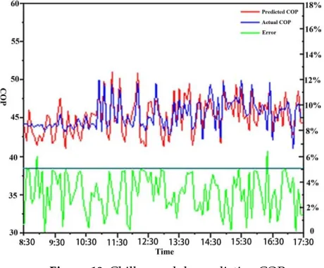
Figure 10. Chiller module prediction COP
338
There are only 2 points where the module prediction COP and the actual COP error are greater
339
than 5%. That is, the COP prediction accuracy of the chiller module is above 95% with a probability
340
342
Figure 11. Chiller module prediction cooling water outlet temperature
343
The module predicts that the cooling water outlet temperature of the chiller is lower than the
344
actual temperature, cause the cooling water does not absorb heat from the outside during modeling,
345
and the actual condensing heat of the chiller is greater than the sum of the chiller power and
346
cooling capacity, so the actual outlet water temperature is high. The cooling water outlet
347
temperature error between the predicted and actual values of the module is between 0.5 and 0.7℃.
348
It can be concluded that the accuracy of the chiller module is high enough and can be used for
349
the following simulation from the above analysis results.
350
4.2.2. Chilled water pump module
351
The method of establishing the water pump module is almost the same as that of the chiller.
352
The required parameters are shown in the Table.10.
353
The relevant operation parameters of water pump include inlet water temperature Ti, outlet
354
water temperature To, flow rate G, frequency k, head H, efficiency η, power N, model
355
identification parameters k, G and control signal S.
356
Table.10. Custom chilled water pump module parameters
357
Parameters Chilled water pump Cooling water pump
Model parameters
Rated power Nch、rated flow Gch、
rated head Hch、model identification
parameters
Rated power Nc、rated flow Gc、
rated head Hc、model
identification parameters
Input parameters G2、k2、S G3、k3、S
Output parameters N2、η2、H2 N3、η3、H3
4.2.3. Cooling tower module
358
The relevant operation parameters of cooling tower include tower inlet temperature Tco, outlet
359
tower temperature Tci, cooling water flow rate Gc, fan frequency k, model identification parameter k,
360
and control signal S.
361
Table.11. Custom cooling tower module parameters
362
Model parameters Rated power Nct、rated flow Gct、rated frequency kct、model identification parameters
Input parameters G3、k4、S
Output parameters N4
4.2.4. Matlab control module
364
According to the chilled station control strategy based on the device contribution rate, the
365
Matlab control module is programmed, and the communication between TRNSYS and Matlab is
366
realized through the COM interface. Matlabt compiles the m file into a COM component, and
367
TRNSYS can directly call the m file. At the beginning of the TRNSYS simulation, TRNSYS will read
368
the simulation start time, end time, and simulation step size of the input file; when calling the m file,
369
TRNSYS simulation pauses and waits for Matlab to process the result. Matlab simulation stops at
370
the end of Matlab processing, and TRNSYS reads the simulation results and continues to simulate.
371
It is done alternately until the end of the simulation.
372
4.3. Chilled station TRNSYS simulation platform
373
Create an empty project, add the selected component to the project, set the parameters of each
374
component according to the previous requirements, connect the components, and establish a
375
simulation platform based on the joint operation of TRNSYS and Matlab.
376
377
Figure 12. Chilled station TRNSYS simulation platform
378
The chilled station TRNSYS simulation platform has been established which can be used to
379
simulate the energy consumption of the chilled station and calculate the SEER based on the optimal
380
control strategy.
381
5. Optimization effect analysis of chilled station based on SEER
382
The chilled station TRNSYS simulation platform was used to simulate the energy consumption
383
of the freezing station from July 1 to September 30 (corresponding to the TRNSYS simulation
384
platform 4344h~6552h), and the SEER based on the device contribution rate was calculated.
385
387
Figure 13. Temporary cooling load simulation result of the test building
388
Temporary energy consumption of the air-conditioning system is shown below.
389
390
Figure 14. Temporary energy consumption of the air-conditioning system
391
The temporary SEER is shown below.
392
393
Figure 15. Temporary energy consumption of the air-conditioning system
394
It can be seen that the SEER is around 2.75 in July/August and fluctuates stably. In September,
395
the SEER is not stable as that in July/August, which results in a decrease in the average SEER value.
396
According to the simulation results of the chilled station, the monthly SEER distribution based
397
on the control strategy of device contribution rate of the test building is shown in the following
398
400
Figure 16. Monthly SEER based on the control strategy of device contribution rate
401
The test building is simulated using a control strategy based on device contribution rate and
402
the results show that the average SEER during the cooling season is 2.88. The highest average SEER
403
is 3.26 in August, and the lowest is 2.22 in September. The value of SEER based on the device
404
contribution rate is 2.15 times of the current SEER, indicating that the control strategy is effective
405
and worthy of further research and promotion.
406
6. Conclusions
407
A new chilled station control strtegy is proposed in this article which is based on the device
408
contribution rate and its TRNSYS model is established to simulate energy consumption. SEER is
409
used as an evaluation index to verify the effectiveness of the control strategy.
410
A mathematical model of "chilled capacity - equipment power" of the chilled station is
411
proposed and established with a correlation coefficient of 0.9917 which is
412
692 . 342 897
. 750 -278 . 26 167
. 351 -157 .
157 -0.0634
4 785
. 0 3 391
. 2 -2 336
. 0
1
N N N N
Q .
413
Matlab is used to find the power value of each device that minimizes the total power input of
414
chilled station in the case of a given cooling capacity. The optimal value of device contribution
415
rate is the same and the chilled station COP increases by 1.80%, 0.96%, and 1.65% with the
416
cooling capacity 1180kW, 1160kW, and 1140kW at this condition. The energy consumption of
417
the chilled station is the smallest when the device contribution rate is the same and the SEER is
418
the highest in the case of a certain amount of cooling capacity.Based on this, the whole
419
frequency conversion control strategy of the chilled station based on the device contribution
420
rate is proposed, and the Matlab control module is loaded into the TRNSYS simulation platform
421
to simulate the test building.
422
The actual SEER of test building is 1.34 during the cooling season. The whole frequency
423
conversion control strategy of the chilled station based on the device contribution rate is
424
applied to TRNSYS platform to simulate energy consumption. The simulation result shows
425
that the average SEER is 2.88 which is 2.15 times of the current value.
426
Acknowledgments: The authors gratefully acknowledge the National Natural Science Foundation of China
427
(numbered 51638003) and the Fundamental Research Funding for Central Universities (numbered
428
DUT17RW118) for the cost of research.
429
Author Contributions: Baogang Zhang contacted the site survey. Chang Sun carried out the mathematical
430
models of equipment and the “cooling capacity – power”, established the chilled station TRNSYS platform.
431
Ming Liu checked and revised the manuscript. Lin Lv participated in field tests.
432
Conflicts of Interest: The authors declare no conflict of interest.
433
References
435
1. Liu G.D.; Ma W.W.; Liu Q.Y. Energy consumption analysis of air conditioning cooling water pumps by
436
variable frequency speed regulation. National HVAC Refrigeration 2010 Annual Conference Proceedings,
437
2010.
438
2. Shuang L. Full-frequency conversion and energy-saving analysis of cold station system. Refrigeration and
439
air conditioning 2015, 35(12), 48-51.
440
3. Bahnfleth W.P.; Peyer E.B. Energy Use and Economic Comparison of Chilled-Water Pumping System
441
Alternatives. ASHRAE transactions 2006, 112(2).
442
4. Fangyuan L. Cooling Tower Fan Frequency Control and Energy Saving. Fan technology 2007. 2, 57-59.
443
5. Thomas Hartman. P.E. New ‘LOOP’ chiller plant uses advanced technologies to achieve big cost
444
reductions. Joint ASHRAE/AEE Technical Seminar, Edmonton, Alberta November, 1999.
445
6. Yang Q.; Zhu J.; Xu X., et al. Simultaneous control of indoor air temperature and humidity for a chilled
446
water based air conditioning system using neural networks. Energy and Buildings 2016, 110, 159-169.
447
7. Chang Y.C.; Chen W.H. Optimal chilled water temperature calculation of multiple chiller systems using
448
Hopfield neural network for saving energy. Energy, 2009, 34(4), 448-456.
449
8. Yang Q.; Zhu J.; Xu X., et al. Simultaneous control of indoor air temperature and humidity for a chilled
450
water based air conditioning system using neural networks. Energy and Buildings, 2016, 110, 159-169.
451
9. Wenping C.; Changzhi Y. and Yuansheng Y. Central air-conditioning water system optimization control
452
based on chiller performance curve. Fluid machinery 2008, 36(8).
453
10. Houjian H. Research on Modeling and Optimization of Central Air Conditioning Water System. Master,
454
Shenyang University of Technology, Shenyang, 2005.
455
11. Zimmer H. Chiller control using on-line allocation for energy conservation]. ISA Annual Conference,
456
Houston, USA, 1976.
457
12. Cho C.H.; Norden N. Computer optimization of refrigeration systems in a textile plant: a case history.
458
Automatica 1982, 18(6), 675-683.
459
13. Braun J.E. Methodologies for the design and control of central cooling plants. Master, University of
460
Wisconsin-Madison, Wisconsin, 1988.
461
14. Braun J.E; Klein S.A.; Beckman W.A. Methodologies for optimal control of chilled water systems without
462
storage. ASHRAE transactions 1989, 95, 652-662.
463
15. Chen C.W.; Chang Y.C. Support Vector Regression and Genetic Algorithm for HVAC Optimal Operation.
464
Mathematical Problems in Engineering 2016.
465
16. Ahn B.C.; Mitchell J.W. Optimal control development for chilled water plants using a quadratic
466
representation. Energy and Buildings 2001, 33(4), 371-378.
467
17. Chen D.D. Study on Real-time Optimization Control Strategy of Central Air Conditioning Variable Water
468
System. Master, Shanghai Jiao Tong University, Shanghai, 2007.
469
18. Zhang L. Research on Energy Saving Reform of a Central Air Conditioning System. Master, Harbin
470
institute of Technology, Harbin, 2013.
471
19. Gao J.; Huang G.; Xu X. An optimization strategy for the control of small capacity heat pump integrated
472
air-conditioning system. Energy Conversion and Management 2016, 119, 1-13.
473
20. Wu S.H. Design and Implementation of Group Control System of Freezing Room. Msater, East China
474
University of Science and Technology, Shanghai, 2014.
475
21. Bursill J.; Cruickshank C.A. Heat Pump Water Heater Control Strategy Optimization for Cold Climates.
476
Journal of Solar Energy Engineering 2016, 138(1), 011011, 10.1115/1.4032144
477
22. Ahn B.C.; Mitchell J.W. Optimal control development for chilled water plants using a quadratic
478
representation. Energy and Buildings 2001, 33(4), 371-378.
479
23. Jia P. Brief Analysis of GB19577-2015 "Cold Energy Efficiency Limit Value and Energy Efficiency Grade of
480
Chillers". Air conditioning HVAC technology 2016, 4, 32-33.
481
24. Yang L.N. Research on Energy Efficiency Ratio of Air Conditioning Projects in Public Buildings. Master,
482
Chongqing University, Chongqing, 2007.
483
25. Zhang B.G.; Wang T.X.; Liu M. Establishment of chilled water system model based on monitoring data.