A Tracker Alignment Framework for Augmented Reality
Yohan Baillot and Simon J. Julier
ITT Advanced Engineering & Sciences
2560 Huntington Ave
Alexandria, VA 22303
{
baillot,julier
}
@ait.nrl.navy.mil
Dennis Brown and Mark A. Livingston
Naval Research Laboratory
4555 Overlook Ave SW
Washington, DC 20375
{
dbrown,markl
}
@ait.nrl.navy.mil
Abstract
To achieve accurate registration, the transformations which locate the tracking system components with respect to the environment must be known. These transformations relate the base of the tracking system to the virtual world and the tracking system’s sensor to the graphics display. In this paper we present a unified, general calibration method for calculating these transformations. A user is asked to align the display with objects in the real world. Using this method, the sensor to display and tracker base to world transformations can be determined with as few as three measurements.
1. Introduction
Almost all Augmented Reality (AR) systems use a track-ing system to capture motion of objects in the real world and map them into the computer generated environment. The most important relationship is head tracking — whenever the user moves their head in the “real world”, the viewpoint in the graphics system should move accordingly. Similarly, if tracked props or interaction devices are moved in the real world, their movements should follow accordingly.
However, registration errors are the result of three error sources:
1. Tracking errors. These occur when the measurement returned by the tracker does not agree with the real pose of the tracker.
2. Display calibration errors. These arise when the op-tical characteristics of the display are unknown. It in-cludes parameters such as field-of-view, distortion and centre of projection. Although these parameters can vary (for example, a camera with a zoom lens), in many applications these parameters are constant and generally it sufficient to calibrate the display once.
3. Tracker alignment errors. The sensor measurements must be transformed so that the graphics are rendered in the display at the correct viewpoint. The transforma-tion requires the knowledge of the world-to-base trans-formation (where is the origin of the tracker coordinate system in the world?) and the sensor-to-manipulator transformation (how is the sensor placed relative to the display?) Although these parameters tend to stay constant with time, they can vary when (1) the tracker base is moved (e.g. the magnetic emiter of a magnetic tracker is moved) (2) the sensor is moved on the HMD (e.g. relocated on the HMD or HMD’s headband ad-justed ).
The alignment problem we are concerned with is to de-termine where the base is with respect to the origin of the virtual world and where the manipulator is with respect to the sensor to which it is attached. Many authors have considered the problems of tracking errors and display er-rors [2, 4, 6–8]. However relatively few authors have con-sidered the problem of tackling the alignment errors. There are many strategies that can be used to find the correct align-ment of the tracker but there are no unified method that can be used for any tracking system.
This is a surprisingly difficult problem for prototyping and developing AR systems. In many systems, a flexible display such as the Sony Glasstron allow the user to fit it correctly to her head. However, every time an adjustment is done the transform between the display and the sensor is changing. In addition it might be necessary to change the location of the sensor on the headband, which pose each time the problem of locating the new sensor with respect to the display.
Figure 1. The problems of tracker alignment are exacerbated when multiple tracking sys-tems are used simultaneously. This mobile system uses an inertial navigation system and a GPS.
and with the display attitude are not known. In addition, the use of an inertial sensor stabilized by compass and a GPS re-quire the knowledge of the frame of references within which these sensors give their measurement. Similar problems oc-cur in hybrid tracking systems where the observations from multiple sensors are fused together in a central estimation algorithm such as a Kalman filter [15].
Early systems, such as those described in [1], often used open-loop calibration. That is, they essentially had to trust the measurement of the location of the tracking system in the environment and on the HMD. Bajura, for example, formed a closed-loop system with a video see-through sys-tem by using the HMD camera to provide direct feedback for the registration [4]. Although this approach solved the sensor to HMD transform, it did not solve the tracker emit-ter to world transform. Furthermore, the approach explicitly assumed a video see-through display and cannot be used for optical see-through display systems. To calibrate its set of trackers (Flock of Birds, Faro mechanical arm, and video cameras), the UNC ultrasound system exploited the fact that the regions of each device overlapped [13]. How-ever, this configuration is highly specialized. Tuceyran pro-posed a calibration method for getting the unknown rigid transforms in the GRASP system [11]. While the method was presented as being applicable to any AR system, it uses a video see-through setup and a tracked pointer as part of the calibration procedure, however this is not the configura-tion of every AR systems. One means of calibrating multi-ple trackers was by basically letting the trackers “overlap” their operating region. Kutulakos and Vallino [10] used a projective world and markers to align the virtual objects
but this setup required a video see-through setup to work. In the general case when a video see-through system is used, there is no need to know the location of the tracker components in the world because the sensor is collocated with the display and the world is collocated with the pattern tracked. Fuhrmann [6] described a method for fast calibra-tion in AR, but the descripcalibra-tion of the method is very suc-cinct and therefore difficult to reproduce and it is not clear that the transform we are concerned with are actually deter-mined. Tuceryan introduced the Single Point Active Align-ment Method (SPAAM) [7, 14] to perform the calibration of an optical see-through HMD. However, this method re-quired many points (minimum 6, recommended 12) to be sighted by one user, and stereo must be used to judge and align correctly the depth, which is a difficult task.
The structure of this paper is as follows. Section 2 de-fines the notation and discusses the problem statement in detail. In Section 3 we consider the problem of calcu-lating the sensor-to-manipulator transformation when the world-to-base transformation is assumed to be known. Sec-tion 4 extends this to the case when neither the sensor-to-manipulator nor the world-to-base transformations are known. The implementation of this framework is outlined in Section 5 and a set of results for a test case are given in Section 6. Summary and conclusions are given in Section 7.
2. Problem Statement
Throughout this paper we use the following notation. Let a referential (or rigid coordinate system) X be written as X. Let XY be the motion or homogeneous transformation that aligns the X referential with a second referential Y1.
Furthermore, from the properties of inverses of transforma-tions, YX= (XY)−1.
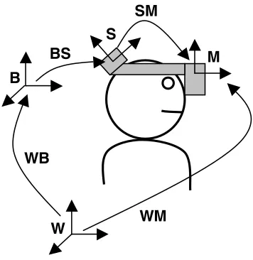
The problem of aligning the head mounted display with the graphics system is illustrated in Figure 2. A user wears a tracked head mounted display. The part of the head mounted display responsible for generating the graphics is fixed to the manipulator with referential M. A sensor with referential S is rigidly attached to the headband of the head mounted display. The sensor base (origin of the tracking system) is B. Therefore, the tracking system actually mea-suresBS. To render the graphics properly, the attitude of the graphics display in the world (WM) must be known.
From the figure, these transformations are given by
WM=WBBSSM. (1)
In other words,WMcan be calculated if the world-to-base (WB) and sensor-to-manipulator (SM) transforma-tions are known. In some situatransforma-tions these quantities can be
1In other words, if the transformation matrix of X isM
M
S
B
W
WM
WB
BS
SM
Figure 2. The referentials and transformations which are relevant for tracker alignment.
determined in advance. However, in some circumstances it can be difficult to determine these quantities in an offline manner.
The sensor-to-manipulator transformation SM can be difficult to calculate for two reasons. The first is that it can be difficult to determine the point at which the measure-ment is made. Sensing devices are of finite size, and it can be difficult to work out the point within the sensor which is being tracked. The second is that the sensor and manipula-tor might not be rigidly attached to one another. The Sony Glasstron, for example, includes a hinged joint which al-lows the display to be translated and rotated with respect to the head band. To counterbalance the weight distribution on the user’s head, it is not always possible to attach the tracker to the display itself but rather to the headband. Therefore, as a user adjusts a display (either during a calibration pro-cedure or even during normal use),SMis changed. Even if the display is fixed with respect to the sensor’s mounting point, the sensor might be installed in a manner such that its transformation with the display is not intuitive2.
At first sight, it might appear that calculating the world-to-base transformationWB is significantly simpler. The prevailing assumption appears to be that this is a fixed, easy to identify and easy to measure property. As a result, with careful measurement, the transformation can be calculated. However, there are two difficulties with this approach. The first is that it is not always possible to accurately measure
2One common practice is to try to mount the trackers as “horizontally
as possible on the display”. Assuming the tracker is horizontal, only the yaw needs to be corrected. However, in general the sensor will not be properly aligned and this leads to coupling of pitch and yaw rotations in highly non intuitive ways.
the base of the tracker in the physical world. In our mo-bile augmented reality work indoor users (who are tracked with by an InterSense IS900) must be able to see and inter-act with outdoor mobile users (whose positions are tracked using a GPS). Therefore, the base of the IS900 must be expressed in world fixed (longitude/latitude) coordinates. However, it is not immediately obvious how this can be cal-culated3. A second problem is that some tracking systems
simply do not have a tangible, physical source which cor-responds to the tracker base. The InterSense InertiaCube 2 (IC2), for example, utilizes magnetometers to constrain the yaw of an orientation tracker. The base of the magne-tometer is magnetic north. However, as is well known, local magnetic anomalies can distort the magnetic field. In effect the sensor base changes as the tracker moves through the environment.
We now describe two calibration procedures. The first calculates SMunder the assumption thatWBis known. The second generalizes this result to determine bothWB
andMS.
3. Single Point Calibration Technique
The single calibration point technique uses a single mea-surement to calculate SM. The technique is built on the observation thatSMcan be calculated by inverting Equa-tion 1:
SM=SBBWWM. (2)
The difficulty with this approach is that the true loca-tion of manipulator, expressed in world coordinates, must be known. Because we are using an optical see-through display, this can be achieved by asking the users themselves to align the contents of the display directly with objects in the environment.
The calibration procedure is illustrated in Figure 3: the environment contains two calibration points — a reference point on the ground (C) and a calibration mark on the wall (G). The locations of these marks must be known within the coordinate system of the model. The display renders graph-ics as if the head mounted display was placed at a known value ofWM. The user is asked to stand on C and align the contents of the display with G. When the two are aligned, the user has positioned the display at the knownWM loca-tion and a tracker sample (a sample ofSB) is recorded.
The transformation WM can be decomposed into a transformation from the world to C, and from C to M:
WM=WCCM. (3)
Under the assumption that C is not rotated4,WCis of the
3Because the tracking system is mounted indoors, GPS cannot be used
to directly measure position.
4This assumption is valid because C specifi es the location of the user’s
M
S
B
W
Calibration mark
Height (H) Cross
WM
WB
BS
SM
C
G
Figure 3. The single point calibration tech-nique. Assuming that the world-to-base transformation is known, the sensor-to-manipulator transformation can be calculated by asking the user to align the contents of the display with appropriate objects in the envi-ronment.
form:
WC=
1 0 0 xwc
0 1 0 ywc
0 0 1 zwc
0 0 0 1
(4)
To calculateCM we use three assumptions. The first assumption is that the user looks directly at G. Therefore, when the display is correctly aligned with the real world, G is projected into the center of the screen5. The second assumption is that that the tracker is aligned such that the roll component is zero. The third assumption that the height of the tracker off the ground,H, is known.
DecomposingCMinto a pure translation and a pure ro-tation,
CM=TcmOcm. (5)
The first component is the vertical translation,
Tcm=
1 0 0 0 0 1 0 0 0 0 1 H
0 0 0 1
(6)
The second component is the rotation needed to align the displays. Using the assumption that the roll angle is zero,
5This is only true if the display is monoscopic. If it is stereoscopic, the
projection is shifted for each eye according to the eye separation.
this can be decomposed into an azimuth rotationψ(about the body-fixedz-axis) followed by an elevation rotation φ (about the body-fixedx-axis)
Ocm=RzRx. (7)
ψandφcan be calculated fromMG.MGis the trans-formation from the manipulator to the calibration mark. The translation(xMG, yMG, zMG)is not a function of the ori-entation. Therefore,
ψ= tan−1−xMG
yMG
φ= sin−1z
MG/ x2MG+yMG2 +zMG2
The resulting procedure is simple and effective. The user is merely asked to stand in a known location and align the contents of the head mounted display with the environment. We have extensively used it in our own system and have ap-plied it to many demonstrations using the system at many different sites. This calibration is easy and allows the flex-ibility to place the sensor anywhere on the user head and with any orientation.
However, this algorithm relies on the assumption that
CM can be calculated. In the approach presented here, this is equivalent to assuming that the height of the display off the ground, H, is known. There are two ways of ad-dressing this problem. The first is to attempt to measure the user height accurately. The second is to place the cali-bration target as far from the user as is practical. However, if more accuracy is required, the SPAAM method could be used [14]. Another possibility is to use a video see-through display looking at a known landmark. In this specific case, the camera is collocated with the graphics referential (the manipulator) and therefore the pose of the camera recov-ered by vision tracking during the calibration phase directly gives the pose of the manipulator. In the case where an op-tical see-through display must be used, a similar approach could be done by rigidly attaching a camera to the display and calibrating the camera to display transformation once for all. We are currently working on such a calibration method6.
6The calibration of the properties of an optical see-through display
W0
B0
W1
B1
S0
M0
S1
M1
B0S0
S0M
S0S1
S1M
M0M1
B0W0
B0B
B1W1
W0W1
B0S1
V0
U1
U0
V1
B1S1
W0M0
W0M1
W1M0
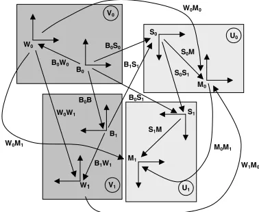
Figure 4. The Multi Point Calibration tech-nique.
Although this approach is effective for cases where the base is known, it cannot be used when the pose of the base is unknown. The next section introduces a method to solve this problem.
4. Multiple Point Calibration Technique
When the world-to-base transformation WB is not known, the single point calibration technique described in the last cannot be used because Equation 2 cannot be eval-uated. However, the necessary information can be gleaned from looking at how therelativetransformations which oc-cur when the user calibrates on a pair of calibration points.
Consider the situation shown in Figure 4: U0and U1 rep-resent the user head that includes the sensor S and manipu-lator M (which in this specific case is the graphical referen-tial). V0represents the rigid group that include the world W and the base of the tracking system B. When the user moves her head between two calibration marks (motion from U0to U1), the sensor produces the motion S0S1and the manipula-tor produces the motion M0M1. S0S1and M0M1are related through the transformationSMbetween the sensor and the manipulator. The problem can be inverted to findBW, the transformation between the base and the world, using no additional motion from the user. In effect, a motion of the head with respect to the world can be seen as a motion of the world with respect to the head. In this case, the head is fixed in U0and the world and tracker base are moving from V0to V1. In this case B0B1and W0W1are related through the transformationBW.
More formally, suppose the user stands at two different locations (C1and C2) and looks at two different calibration marks (G1 and G2). The sensor referentials in these two
locations are S1 and S2, and the manipulator referentials are M1and M2.
Writing out Equation 2 for each measurement,
SM=S1BBWWM1 (8)
SM=S2BBWWM2. (9)
Rearranging Equation 8,
BW=BS1SMM1W.
Substituting into Equation 9,
SM=S2BBS1SMM1WWM2.
Postmultiplying both sides byM2WWM1gives
(S1BBS2)SM=SM(M1WWM2). (10)
This is exactly the same as the so-called “hand-eye” cal-ibration framework problem which is frequently encoun-tered in robotics [12]. In a typical robotics application, a manipulator is rigidly attached to the actuator. The transfor-mation from the actuator to the manipulator is not known. However, both the actuator and the manipulator contain tracking systems. In a typical configuration, the actuator might be a robotic arm (whose geometry is known and whose joint angles are measured) and the manipulator con-tains a camera. The problem is conventionally posed as
AX=XB (11)
whereAis the motion of the first referential,Bis the mo-tion of the second referential, andXis the transformation that aligns the first referential with the second one.
If A andB could be measured perfectly, solving this equation would be a trivial linear algebra problem. How-ever, because A and B are measured by noise-corrupted sensors, more sophisticated techniques must be used to en-sure that X is a properly formed homogeneous transfor-mation matrix. Within the robotics literature, a number of different approaches have been proposed. For this pa-per we used a closed-form solution developed by Park and Martin [5] . This solution, described in detail in the ap-pendix, uses Lie Bracketing Algebra and matrix logarithms and yields an extremely compact and easy to implement so-lution.
A similar approach can be taken to solveWB. Substi-tuting Equation 8 into Equation 9,
S1BBWWM1=S2BBWWM2.
Premultiplying byBS2and post multiplying byM1W,
(BS2S1B)BW=BW(WM2M1W). (12)
Once again, this is in the form of the ”hand-eye” calibra-tion problem and can be solved in exactly the same man-ner7.
5. Implementation
The calibration framework described in the previous sec-tion was implemented within the Battlefield Augmented Re-ality System (BARS) [9]. The interactive authoring system described in [3] was extended to allow users to annotate an environment model with a set ofN calibration cross refer-entials Ciand calibration marks Gi.SMiis calculated from Equation 3 for each Ci/Gipair.
When solving Equations 10 and 12, it is possible to ex-ploit the fact that Equations 8 and 9 apply foranypair of relative transformations. For example, when solving Equa-tion 10, it is possible to constructN(N−1)/2equations of the form
(SiBBSj)SM=SM(MiWWMj).
where i, j ∈ [1, . . . , N]andi = j. As shown in the ap-pendix, this can greatly increase the performance of the so-lution.
We now demonstrate the use of this approach at a test environment.
6. Example
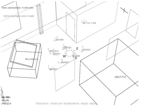
The alignment framework was used to align the sensors in an indoor mobile augmented reality system. The geo-metric model of the environment is shown in Figure 5 — the environment consists of a single room and a number of pieces of laboratory equipment. The model has been aug-mented to include the calibration crosses (thenth cross is labeledAXXBn) and the calibration marks. Most of the cal-ibration marks in this model are preexisting features such as the corners of doors or walls. One artificial calibration mark, a cross, can be see on the right of the picture.
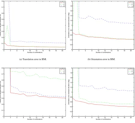
A set of 7 calibration crosses and calibration marks were created. To test the effectiveness of this configuration, a sensitivity analysis was performed using a Monte Carlo analysis. It was assumed that the measurement error (which includes tracker error and misalignment errors by the user) has a standard deviation of 0.05m in position and 0.5 de-grees in orientation8. Figures 6(a) and 6(b) show the 2σ
standard deviation of the error inSM. These plots show that the2σerror inSMis between 0.05m (X and Z) and 0.15m (Y), and the orientation error is between0.5◦(X and Y) and1.2◦(Z). We believe that the errors in Y (for posi-tion) and Z (for orientaposi-tion) are much larger as a result of the calibration configuration which was used — namely that all of the calibration marks were at approximately the same
assume that the tracker base B is fi xed and allow the manipulator M to move. To solve forWB, we assume that M is fi xed and allow B to move.
8Positions are given in metres. Orientations are expressed in Euler
an-gles using rotation about fi xedXY Zaxes (the same convention is used by Java3D).
Figure 5. The sample calibration environment.
height. The simulation studies confirm that, with a more uniform distribution of marks in three-dimensions, the er-rors in all rotation angles and positions decrease at approx-imately the same rate.
The figures also illustrate that, as the number of com-binations increase, the magnitude of the error is reduced. Figures 6(c) and 6(d) show the standard deviations of the errors in translation and orientation of WB. The results are very similar to those forSM: the error on the position were ranging between 0.35 and 0.7m, and the error on the orientation were ranging between0.4◦and1.2◦.
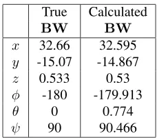
These measurements were confirmed by conducting an actual calibration experiment. The tracking system is an In-terSense IS900LAT. The user stood at each of the 7 calibra-tion points and was asked to align the display with the ap-propriate calibration mark. Through careful (and laborious) measurement, the value of WBwas accurately obtained. Table 1. As can be seen, the results are extremely accurate for almost all results and are, in fact, significantly better than those predicted by the covariance analysis. In this ex-perimental configuration,SMcould not be accurately mea-sured independently. However, because observed registra-tion errors in the calibrated display were small, we believe that it was estimated accurately.
7. Conclusions
2 4 6 8 10 12 14 16 18 20 0
0.1 0.2 0.3 0.4 0.5 0.6 0.7 0.8
Number of combinations
Position error standard deviation (m)
x y z
(a) Translation error inSM.
2 4 6 8 10 12 14 16 18 20
0 0.2 0.4 0.6 0.8 1 1.2 1.4 1.6 1.8 2
Number of combinations
Orientation error standard deviation (deg)
φ θ ψ
(b) Orientation error inSM.
2 4 6 8 10 12 14 16 18 20
0 0.1 0.2 0.3 0.4 0.5 0.6 0.7 0.8
Number of combinations
Position error standard deviation (m)
x y z
(c) Translation error inBW.
2 4 6 8 10 12 14 16 18 20
0 0.2 0.4 0.6 0.8 1 1.2 1.4 1.6 1.8 2
Number of combinations
Orientation error standard deviation (deg)
φ θ ψ
(d) Orientation error inBW.
True Calculated
BW BW
x 32.66 32.595
y -15.07 -14.867
z 0.533 0.53
φ -180 -179.913
θ 0 0.774
ψ 90 90.466
Table 1. The calculated and true values of the base-to-world transformation.
of calculating the sensor-to-manipulator and world-to-base transformations in the same step.
We shall extend this calibration method in the following ways:
• Develop tools that will provide user with feedback in designing a calibration scheme. For example, the algo-rithm we used to solve the hand-eye calibration prob-lem cannot be applied if the trace of any transforma-tion matrix is -1. Such conditransforma-tions can be detected as the marks and crosses are being created and surveyed in.
• Explore schemes to automatically optimize the place-ment of calibration marks to improve the accuracy of the calibration result, based on using this tool and un-derstanding in which situations the logarithm fails.
• Explore the effect of other solvers to see how these are affected by noise and / or marker placement.
• Use this algorithm to solve the relative placement of two trackers used to form an hybrid tracker.
A. Solving the Calibration Equations
The calibration framework relies on the ability to solve the equation
AX=XB (13)
whereA,BandXare transformation matrices. This prob-lem is extremely important in the field of robotics where it is known as the “hand-eye” calibration problem. Given a set ofNmeasurements ofAandB, findXsuch that
A1X = XB1 ..
. ...
AN X = XBN
A number of different solutions have been developed for this problem. Most of these solutions are iterative, and are
typically designed for automatic systems where many hun-dreds of samples can be taken. Accurate solvers which re-quire few measurements are extremely important.
For this paper, we used an approach which was devel-oped by Park and Martin in [5]. Despite the theoretically complexity of the algorithm (it is based on the matrix log-arithm of the transformation matrix) it is extremely easy to implement.
LetΘ∈SO(3)be any rotation matrix and letb∈R3be the translation. Therefore, any valid transformation matrix
Mhas the form
M=
Θ b
0 1
.
If trace[Θ]=−1, the logarithm of this matrix is
logM=
[ω] A−1b
0 0
where[ω] = logΘandAis a matrix whose is irrelevant for solving the calibration problem.
Letφbe
φ= cos−1trace[Θ]−1 2
(14)
The matrix logarithm[ω]is
[ω] = φ 2 sinφ
Θ−ΘT (15)
This is a skew symmetric matrix
[ω] =
ω03 −0ω3 −ωω21
−ω2 ω1 0
. (16)
Therefore, [ω] can be parameterised as the vector ω where
ω=
ωω12
ω3
Letαibe the matrix logarithm of measurementAiand
βibe the matrix logarithm of measurementBi.
The Park-Martin algorithm [5] attempts to findX
X=
ΘX bX
0 1
.
The algorithm decomposes the solution into two sub-problems. The first is to calculate the rotation ofΘX. This can be carried out independently of the translations. The second problem calculatesbXusing the calculated value of
ΘX
The rotation matrixΘX is chosen to minimise the cost function
η1=
p
i=1
The optimal solution is
ΘX=MT M−1/2MT (18)
where
M=
p
i=1
βiαT
i. (19)
If p = 2, the third measurements are synthesised as
α3=α1×α2andβ3=β1×β2.
The matrixMhas the property that it isalways guaran-teed to be orthonormal even if the data is noisy.
The second optimisation solution minimises
η2=
p
i=1
||(ΘAi−I)bX−ΘXbBi+bAi||2. (20)
This can be expressed as a standard least squares min-imisation problem and its solution is
bX =CTC−1CTd
where
C=
I−ΘA1 .. .
I−ΘAp
and
d=
bA1−ΘXbB1 .. .
bAp−ΘXbBp
.
This equation can be solved even if only 2 measurements are used.
References
[1] R. T. Azuma. A survey of augmented reality. Pres-ence: Teleoperators and Virtual Environments, 6(4):355– 385, 1997.
[2] R. Azuma, G. Bishop. Improving static and dynamic regis-tration in optical see-through hmd. InProceedings of SIG-GRAPH’94, pages 197–204, July 1994.
[3] Y. Baillot, D. Brown, and S. Julier. Authoring of Physical Models Using Mobile Computers. InProceedings of Inter-national Symposium of Wearable Computers, 2001. [4] M. Bajura and U. Neumann. Dynamic registration
correc-tion in video-based augmented reality systems. IEEE Com-puter Graphics and Applications, (5):52–60, 15 1995. [5] F.C. Park and B. Martin. Robot Sensor Calibration:
Solv-ing AX=XB on the Euclidean group.IEEE Transactions on Robotics and Automation, 10(5):717–721, October 1994. [6] A. Fuhrmann, D. Schmalstieg and W. Purgathofer. Fast
Calibration for Augmented Reality. InProceedings of the ACM Symposium on Virtual Reality Software and Technol-ogy, pages 166–167, London, UK, 20–22 December 1999.
[7] Y. Genc, M. Tuceryan, and N. Navab. Pratical Solution for Calibration of Optical See-Through Devices. In Proceed-ings of International Symposium of Mixed and Augmented Reality, 2002.
[8] A. Janin, D. Mizell, and T. Caudell. Calibration of head-mounted display for augmented reality applications. In Pro-ceedings of Virtual Reality International Symposium, 1993. [9] S. Julier, Y. Baillot, M. Lanzagorta, D. Brown, and L.
Rosenblum. BARS–Battlefi eld Augmented Reality System. InNATO Symposium on Information Processing Techniques for Military Systems, 2000.
[10] K. N. Kutulakos and J. R. Vallino. Calibration-free aug-mented reality. IEEE Transactions on Visualization and Computer Graphics, 4(1), – 1998. ISSN 1077-2626. [11] D. M. Tuceryan. Calibration requirements and procedures
for a monitor-based augmented reality system.IEEE Trans-actions on Visualization and Computer Graphics, 5(3):255– 273, 1995.
[12] Y. C. Shiu and S. Ahmad. Finding the Mounting Position of a Sensor by Solving a Homogenous Transform Equation of the FormAXequalsXB. InProceedings of the IEEE In-ternational Conference on Robotics and Automation, pages 1666–1671, Raleigh, NC, USA, 1987.
[13] A. State, G. Hirota, D. T. Chen, W. F. Garrett and M. A. Livingston. Superior augmented reality registration by inte-grating landmark tracking and magnetic tracking. In SIG-GRAPH 96 Conference Proceedings, Annual Conference Series, pages 429–438. ACM SIGGRAPH, Addison Wesley, 1996.
[14] M. Tuceryan, and N. Navab. Single Point Active Alignment Method (SPAAM) for Optical See-Through HMD Calibra-tion for AR. InProceedings of International Symposium of Augmented Reality, 2000.