A Practical Method for Explicitly Modeling Quotas and Other Complementarities

Full text

(1)Eleventh Floor Menzies Building PO Box 11E, Monash University Wellington Road CLAYTON Vic 3800 AUSTRALIA. CENTRE of POLICY STUDIESand the IMPACT PROJECT. Telephone: (03) 9905 2398, (03) 9905 5112. from overseas: 61 3 9905 5112 or 61 3 9905 2398. Fax: (03) 9905 2426 e-mail. 61 3 9905 2426 [email protected]. web site. http://www.monash.edu.au/policy/. th. Paper presented at the 5 Conference on Global Economic Analysis Taiwan, June 2002. A PRACTICAL METHOD FOR EXPLICITLY MODELING QUOTAS AND OTHER COMPLEMENTARITIES. by. W. Jill HARRISON, Mark HORRIDGE, K.R. PEARSON and Glyn WITTWER. Centre of Policy Studies, Monash University. Preliminary Working Paper No. IP-78 April 2002. ISSN 1 031 9034. ISBN 0 7326 1531 3. The Centre of Policy Studies (COPS) is a research centre at Monash University devoted to quantitative analysis of issues relevant to Australian economic policy..

(2) ABSTRACT To make CGE models realistic, we sometimes need to include inequality constraints (eg, import quotas) or non-differentiable functions (eg, income tax schedules). Both situations may be described using complementarity conditions, which state that either an equation is true or its complementary variable is at a boundary value. The paper describes a practical way to solve CGE models, which contain such conditions. The technique, which is different from complementarity algorithms commonly used elsewhere (eg GAMS), has been implemented for the next version of the GEMPACK system. In the Euler (and similar) methods used by GEMPACK, derivatives are calculated to work out the approximate effects of exogenous changes. To get more accuracy, we can divide exogenous changes into several smaller steps. We interpret this procedure as a path-following algorithm. If all equations in the model are smooth (have continuous derivatives) we can always choose sufficiently many steps to be sure that approximation errors are a smooth and decreasing function of the number of steps. At this point we can invoke extrapolation procedures which use results from, say, Euler computations of 10, 15 and 20 steps, to compute results which are as accurate as machine precision allows. The extrapolation also allows us to compute error bounds for our computation. Unfortunately, complementarity conditions are equivalent to kinked schedules; they contain points where derivatives change sharply. The lack of smoothness precludes the use of extrapolation. Without extrapolation, very many tiny Euler steps might be needed to ensure sufficient accuracy— leading to unacceptably lengthy computations. Our paper describes one way of overcoming this problem. The key insight is that if we knew in advance which constraints would be binding in the accurate solution, the complementarity conditions could be reformulated in terms of smooth functions only, via a closure change which allows us to ignore the troublesome equations. With all remaining functions smooth, extrapolation again becomes effective. This leads to a two-pass procedure. First, a single Euler computation, of limited accuracy, is used to discover which constraints will finally bind. Using this information the equations are recast into an equivalent smooth system which is then solved accurately. Similar methods have been used in Australia and elsewhere for years. They are simple and intuitive—but tedious and difficult to implement manually, especially where many complementarity conditions interact. GEMPACK now offers a syntax for expressing complementarity conditions in a standard way. This enables the software to take over the boring work: running the approximate simulation, making the closure change and identifying target values for the newly exogenous variables, and finally re-solving accurately. We illustrate the technique with WAYANG, a SAM-based CGE model of Indonesia. Here, import quotas yield large rents to some richer households. We expect that removing the quotas should improve income distribution. However, the simulation results contain some surprises. KEY WORDS: complementarity, applied general equilibrium, quotas, tariff-rate quotas, inequality constraints, algorithm.

(3) 15:16 10.05.02. CONTENTS 1. Introduction 1.1. How inequality constraints and non-differentiable functions arise in realistic models. 1 1. 1.2. Complementarity conditions: a standard way to formulate inequality constraints and non-differentiable functions 2 2. The standard GEMPACK path-following algorithm. 3. 2.1. The Euler approach. 3. 2.2. Why the Euler method is so efficient for CGE models. 5. 2.3. How extrapolation gives high accuracy at little cost. 6. 2.4. The Euler technique with a complementarity. 6. 2.5. Why extrapolation does not work with complementarity conditions. 7. 2.6. Path following a generalized complementarity. 8. 2.7. If only we knew which constraint would finally bind. 9. 3. A two-pass method for accurately solving models containing complementarity conditions. 9. 3.1. Making the initial approximate simulation more efficient Newton corrections to jump back towards the complementarity Variable step length to minimize overshooting. 9 9 10. 3.2. Precursors of the latest GEMPACK implementation Try-it-and-see closure swapping Newton-assisted path following in Euler context Newton path following in a levels model Specialized ancillary programs to automate closure swapping Today: a generalized treatment integral to GEMPACK. 11 11 11 11 11 12. 3.3. Specifying a complementarity in GEMPACK. 12. 3.4. How GEMPACK treats complementarities during a simulation. 14. 4. Illustration from Indonesia: effects on equity of cutting quota rents. 15. 4.1. The WAYANG model. 15. 4.2. The simulation Summary of closure. 16 16. 4.3. Results. 16. 5. Conclusion. 18. REFERENCES. 18.

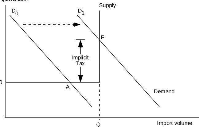
(4) A practical method for explicitly modeling quotas and other complementarities. 1. 1. Introduction This paper describes how the small-change approach to solving CGE (computable general equilibrium) models may be extended to cater for models containing inequality constraints or nondifferentiable functions. Our algorithm is efficient and robust. In layman’s terms, we can say that, like many other algorithms, when it works, it works well. Too often, however, fine algorithms fail to find solutions. Often, the modeler is to blame. Mistakes in data, equations, or exogenous settings lead to equation systems which are indeterminate or insoluble, thus confounding the best solution methods. It may be hard to pinpoint the cause of a solution problem. Error diagnostics can seem unhelpful, especially if they relate to a complex solution algorithm one does not understand. The approach we describe below has a powerful advantage: it is simple and intuitive. The modeler can understand what is going on, and see when (and why) things go wrong. Our exposition aims to highlight this advantage. The remainder of the paper is organized as follows. Section 1 shows how inequality constraints may arise in practice and sets out a general definition of a complementarity, which encompasses inequality constraints as well as other non-differentiable functions. In Section 2 we describe the Euler algorithm used by GEMPACK (see Harrison and Pearson, 1996), and show why complementarity conditions reduce its efficiency. Section 3 describes a modified Euler method which efficiently solves models containing complementarities. We list some details of the GEMPACK implementation. Section 4 illustrates the new technique using a CGE model of Indonesia: we simulate the removal of an import quota. We conclude in Section 5. Investment. 0. A. Rate of Profit. Figure 1: Investment related to profit rate. 1.1. How inequality constraints and non-differentiable functions arise in realistic models Most of the equations in a typical CGE model are numerically well-behaved, smooth functions with continuous derivatives. Linear relations abound, such as accounting or market-clearing conditions. Common functional forms, such as CES demand functions, yield always-positive input demands, which depend on price ratios, which are also naturally positive. Yet, optimizing behaviour is occasionally bound by non-negativity constraints. For example, in a dynamic model, the desired level of capital may decline too quickly to be accommodated by positive investment. So, for a few periods, capital will be greater than desired and investment will be zero, until depreciation reduces stocks to the desired level. The relation, for some industry, between investment and the rate of profit is.

(5) Harrison, Horridge, Pearson and Wittwer. 2. shown in Figure 1. The kink—or discontinuous derivative—at point A gives trouble to many equation-solving algorithms. More often, kinked relations arise from non-market institutions. For example, a tax schedule, relating income to the rate of income tax, will often be composed of several straight-line segments. Again, import quotas may be interpreted as an implicit tax (quota rent) which cuts in only at a certain level of imports—and increases automatically to constrain import demand to that level. The relation between the implicit quota tariff and import volumes is shown in Figure 2. Quota tariff Supply D 0. D1. F. Implicit Tax 0. A. Demand. Q. Import volume. Figure 2: An import quota and associated implicit tariff. Initially the demand curve D0 cuts the import supply schedule at A, where volume is below quota and world prices apply. A rightward shift in demand to D1 results in a new equilibrium F. Here the user price of imports must exceed world prices to hold demand down to the quota level Q. The difference between world and user prices—or implicit tariff—gives rise to quota rents which will accrue to holders of import licences.. 1.2. Complementarity conditions: a standard way to formulate inequality constraints and non-differentiable functions Relations such as those depicted in Figures 1 and 2 may be described in a standard way using complementarity conditions, which state that either an equation is true or its complementary variable is at a boundary value. If X is a variable and EXP is an expression, a simple complementarity is often written X >= 0 ⊥ EXP which is notation for: Either X > 0 and EXP = 0 or X = 0 and EXP >= 0. To represent the import quota of Figure 2 we could set: X = Quota Tariff EXP = Q - Import Volume GEMPACK supports a more general specification of a complementarity: L <=X<=U ⊥ EXP meaning that: (1) Either X = L and EXP>0 (2) or L<=X<=U and EXP=0 (3) or X=U and EXP < 0..

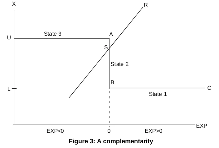
(6) A practical method for explicitly modeling quotas and other complementarities. 3. If desired, only one of the bounds L or U need be specified. This definition of a complementarity is the same as that used elsewhere (eg, section 5 of Ferris and Kanzow (2000), where they define a Mixed Complementarity Problem). Figure 3 depicts a complementarity of this general type as the stepped path UABC. Other model equations are summarized by the sloping line R. The intersection point S is the current solution. According to which of (1), (2) or (3) above is true, we say that the complementarity is in one of states 1, 2 or 3: the point S in Figure 3 is in state 2. Both R and the complementarity schedule may move as other system variables change. R must be positively sloped to ensure a definite single solution. X. U. R. State 3. A S State 2 B C. L State 1. EXP<0. 0. EXP>0. EXP. Figure 3: A complementarity. 2. The standard GEMPACK path-following algorithm GEMPACK draws on a family of related solution methods, including the Euler, Gragg and midpoint methods of solving initial value problems1. Below we briefly describe the Euler method, which is representative of the others. Our aim is to: • briefly describe how Euler works; • list some of its advantages, particularly for large and complex CGE models; and • show how Euler is compromised by complementarity conditions. These points underpin and motivate Section 3, where we describe a modified Euler approach which can cope with complementarities, whilst retaining the Euler advantages.. 2.1. The Euler approach A typical CGE model can be represented as: F(Y,X) = 0, (1) where Y is a vector of endogenous variables, X is a vector of exogenous variables and F is a system of non-linear functions. The problem is to compute Y, given X. Normally we cannot write Y as an explicit function of X. The linearized approach starts by assuming that we already possess some solution to the system, {Y0,X0}, i.e., F(Y0,X0) = 0. (2) 1. See, for example, Pearson (1991), chapter 6 of Atkinson (1989), and chapter 15 of Press et al (1986)..

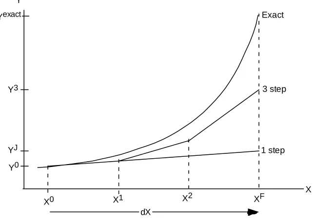
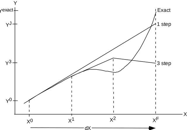
(7) Harrison, Horridge, Pearson and Wittwer. 4. With conventional assumptions about the form of the F function it will be true that for small changes dY and dX: (3) FY(Y,X)dY + FX(Y,X)dX = 0, where FY and FX are matrices of the partial derivatives of F with respect to Y and X, evaluated at {Y0,X0}. Such systems are easy for computers to solve, using standard techniques of linear algebra. But they are accurate only for small changes in Y and X. Otherwise, linearization error may occur. The error is illustrated by Figure 4, which shows how some endogenous variable Y changes as an exogenous variable X moves from X0 to XF. The true, non-linear relation between X and Y is shown as a curve. The linear, or first-order, approximation: dy = - FY(Y,X)-1FX(Y,X)dx (4) J exact leads to the 1-step or Johansen estimate Y —an approximation to the true answer, Y . Y Yexact. Exact. Y3. 3 step. YJ. 1 step. Y0. X0. X2. X1. XF. X. dX. Figure 4: Johansen and Euler approximations. To get more accuracy, we can divide the exogenous change dX into several smaller steps. For each sub-change in X, we use the linear approximation to derive the consequent sub-change in Y. Then, using the new values of X and Y, we recompute the derivative matrices FY and FX. The process is repeated for each step. If we use 3 steps (see Figure 4), the final value of Y, Y3, is closer to Yexact than was the Johansen estimate YJ. We can show, in fact, that given sensible restrictions on the derivatives of F(Y,X), we can obtain a solution as accurate as we like by dividing the process into sufficiently many steps. It is not always true that more steps give more accuracy. In Figure 5, the 1-step (or Johansen) approximation happens to be more accurate than the 3-step result. However, if F has continuous derivatives, there will be some minimum number of steps, Nmin, beyond which accuracy does always increase with the number of steps. In Figure 5, if we took a large enough number of tiny steps, we would get a solution that was more accurate than the Johansen solution..

(8) A practical method for explicitly modeling quotas and other complementarities. 5. Y Yexact. Exact. YJ. 1 step. Y3. 3 step. Y0. X0. X2. X1. XF. X. dX. Figure 5: A few more steps sometimes reduces accuracy. 2.2. Why the Euler method is so efficient for CGE models The simple Euler technique described above has limitations as a general-purpose equation-solving technique. It requires an initial solution and wanders away from the solution path. Nevertheless some special properties of CGE models make Euler very attractive: (a) For most CGE models, an initial solution is readily available, or can be easily constructed. A CGE database contains tables of values—such as input-output tables, which show expenditures on different commodities by various users—and behavioural elasticities which are often constant. Quantities may be deduced from values via an arbitrary choice of physical units—eg, by assuming all prices to be initially unity. (b) Most CGE models can be expressed very simply in log-linear form. We can rewrite (3) above as: GY(Y,X)y + GX(Y,X)x = 0, (5) where y and x are vectors of percentage or proportional changes. Models implemented in GEMPACK are usually specified by writing down (5). The formulae for the coefficients G tend to be very simple and quick to compute: most elements of G are simply transaction values from the CGE database. The simplicity derives from various homogeneity properties of CGE models which in turn arise from the irrelevance of the choice of physical or monetary units. As a bonus, casting the equations into the dimensionless percent-change form avoids many of the scaling problems that can plague solution algorithms. (c) Unlike Newton or other algorithms incorporating a corrector step, Euler does not require us to compute the vector of values of the original function F. This is fortunate, since F tends to be more costly to compute than G. (d) Realistic CGE models tend to be large, often containing millions of (rather simple) equations. Even linear systems of such size are expensive to solve. We must systematically substitute out equations and variables to reduce the system to a manageable size. For a linearized system such as (5) the substitutions can easily be done automatically by software, allowing us to code the model in its simpler, uncondensed, form. Automatic substitution is not generally practical for the original levels system (1); instead, the model must be originally specified in condensed form..

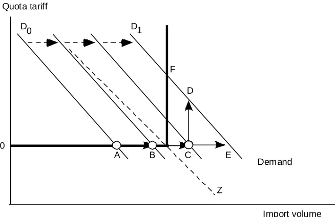
(9) Harrison, Horridge, Pearson and Wittwer. 6. For the above reasons, specification2 in percent-change form and solution using Euler (or related) algorithms are the methods of choice for larger and more complex CGE models. This is the area where GEMPACK predominates.. 2.3. How extrapolation gives high accuracy at little cost As a rule of thumb, we can double the accuracy of an Euler computation by doubling the number of steps. Still, many steps (and much patience) might be needed to ensure sufficient accuracy. To save time we can invoke extrapolation procedures which use results from, say, Euler computations of 3, 6 and 9 steps, to compute highly accurate results. The extrapolation also allows us to compute error bounds for our computation. The extrapolated result requires 18 (= 3+6+9) steps to compute but would normally be more accurate than that given by a single 18-step computation. Alternatively, extrapolation enables us to obtain given accuracy with fewer steps. Note that the first, quickest, of the three Euler computations, should have at least Nmin (see section 2.1) steps. Actually, 2 Euler computations—say, of 6 and 9 steps—would be enough to compute an extrapolated solution. We do 3 Euler computations (3-6-9) so that we can compare results from the 3-6 extrapolation with those from the 6-9 extrapolation. Such comparisons enable the GEMPACK software to establish (rather conservative) error bounds for the extrapolated solutions. From these error estimates we might conclude that more Euler steps (perhaps 6-9-12) are necessary to obtain a sufficiently accurate solution. Thus extrapolation not only makes results more accurate, but, equally importantly, tells us how accurate they are.. 2.4. The Euler technique with a complementarity Quota tariff D 0. D1. F D. 0 A. B. C. E. Demand. Z Import volume. Figure 6: Path-following around a kink. Figure 6, which is based on Figure 2, shows how we could use the Euler procedure to track a complementarity relation. As in Figure 2, demand is moving right from D0 to D1. In this example we assume that the import supply schedule (shown heavy) does not move. The initial equilibrium is at A. A one-step linear approximation that used the slope at A would lead us to the point E, where volume is well above quota. 2. Some GEMPACK veterans, long accustomed to writing down their models directly in percent-change form, claim that the spare elegance of log-derivatives yields both aesthetic and conceptual benefits. They feel that they understand CGE models better by thinking in percentage changes. GEMPACK allows the rest of us to specify the model in the levels, or even in a mixture of levels and change equations. The software automatically translates levels equations into change form as part of the solution process..

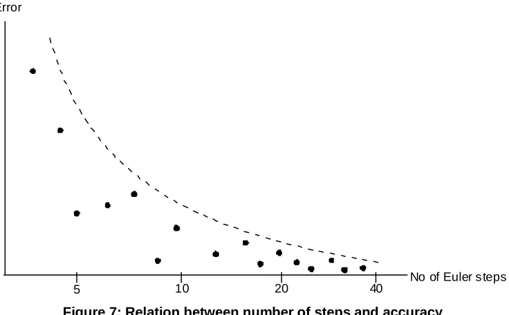
(10) A practical method for explicitly modeling quotas and other complementarities. 7. A 3-step Euler approximation, which divided the demand shock into 3 equal parts, would follow the path ABCD. The second step, BC, still overshoots the quota, but by less than the one-step approximation E. The CD step follows the slope of the vertical (quota-constrained) part of the import supply schedule. The final result, D, is a better approximation to the true result F, than is the onestep approximation E. The Euler procedure requires that we can evaluate derivatives of each equation even for variable values that do not satisfy that equation (eg, in Figure 4 slopes are evaluated at points off the true path). For complementarity equations we must establish a rule to evaluate the slope at points where such equations are not satisfied. The 45-degree dashed line Z indicates this rule. For all points below and left of Z, we assume that the slope of the complementarity is horizontal. For all other points, above and right of Z, we assume that the slope is vertical. Inaccuracy in the Euler solution arises from the overshooting in the BC step. Since the amount of overshooting cannot exceed the length of the entire step, it is clear that by subdividing the shock into very many tiny steps, we can reduce the inaccuracy to any desired level. Figure 7 illustrates the relation between more steps and errors: it is generally, but not uniformly decreasing. The dotted curve indicates the maximum possible error; it is proportional to step length. The accuracy of a particular Euler solution will depend on how close is point C in Figure 6 to the kink—a matter of luck. By contrast, for smooth functions we would find that more steps would always lead to more accuracy—at least for step count >Nmin. Error. No of Euler steps 5. 10. 20. 40. Figure 7: Relation between number of steps and accuracy. 2.5. Why extrapolation does not work with complementarity conditions Figure 7 leads us to a disappointing conclusion. Although Euler can yield accurate solutions in cases like Figure 6, we cannot use extrapolation. The reason is that, however large is the number of steps, N, we cannot be sure that N+M steps will yield a more accurate solution. That is, the number Nmin mentioned above may not exist (as it must when functions are smooth). Without extrapolation, very many tiny Euler steps might be needed to ensure sufficient accuracy—leading to unacceptably lengthy computations. Furthermore, extrapolation is needed to provide the error bounds which reassure us that we have done enough Euler steps to get a solution sufficiently accurate for our purpose. The rest of the paper explains our key innovation: a way to recover the useful extrapolation capability even in the presence of complementarity conditions..

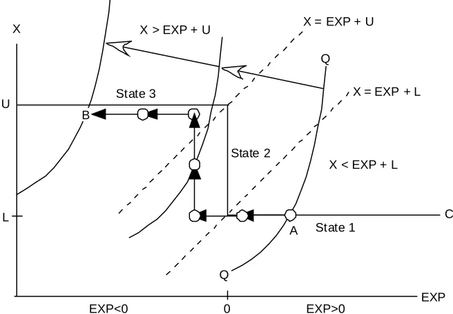
(11) Harrison, Horridge, Pearson and Wittwer. 8. 2.6. Path following a generalized complementarity Figure 8 is akin to Figure 6, but shows how a 6 step Euler could approximately solve a more general complementarity, depicted by the stepped line UC. The initial solution, A, is where UC crosses the curve QQ (representing the rest of the model). A is in state 1: X is at its lower bound L and the complementary expression EXP is positive. As a result of some shock to the system, QQ moves to the left, causing EXP to decrease and eventually become negative. This causes X to increase, eventually reaching point B which is in state 3: X is at its upper bound U and the complementary expression EXP is negative. Along the way the algorithm passes through state 2, where EXP=0 and L<X<U. The dotted diagonal lines divide the plane into 3 zones corresponding to the three states. As in Figure 6, inaccuracies arise when a zonal boundary is crossed, due to overshooting.. X. X = EXP + U. X > EXP + U. Q X = EXP + L. State 3. U. B State 2 X < EXP + L. C. L. State 1. A. Q EXP EXP<0. 0. EXP>0. Figure 8: Tracking a generalized complementarity. X. X > EXP + U Q. U. State 3. Z. B. State 2 X < EXP + L. ∆X. A. L. State 1. Q EXP EXP<0. 0. EXP>0. Figure 9: It’s easier to ignore the complementarity.

(12) A practical method for explicitly modeling quotas and other complementarities. 9. 2.7. If only we knew which constraint would finally bind The complexity of Figure 8 would be greatly reduced if we happened to know in advance in which state the complementarity condition would end up. Figure 9 represents this fortunate situation. Since we know we start in state 1 (X=L) and end in state 3 (X=U) we can drop3 the complementarity condition and instead exogenously shock X by an amount U-L. By dropping the complementarity condition, we can again claim that our equation system consists only of smooth curves, and so restore the desirable extrapolation properties of the Euler procedure: efficiency, accuracy, and known error bounds. Figure 9 still includes the dotted lines which divide the plane into the 3 states of the complementary. Their continued presence emphasizes that, after Euler extrapolation, we can test our assumption about the final state of the complementarity. Point B, the accurate solution, is indeed in State 3 (X=U and EXP<0). If instead we had arrived at point Z (in state 2), our initial assumption (that we end in state 3) would be proved wrong.. 3. A two-pass method for accurately solving models containing complementarity conditions Following the method suggested above, GEMPACK now uses a two-pass method to accurately solve models containing complementarity conditions: (1) The approximate simulation: A single Euler computation, of limited accuracy, is used to discover which constraints will finally bind. This computation follows the pattern of Figure 8. (2) The accurate simulation: Using the results from (1) to predict which constraints will finally bind, we can replace each complementarity condition with one of the equations: X=U, X=L, or EXP =0. The modified system has continuous derivatives and so can be accurately solved using standard GEMPACK methods. The software automatically sets up and runs both simulations as a single job. It is of course conceivable that, after solving the modified system (2) accurately, we discover that not all complementarity conditions are satisfied. That is, the initial simulation (1) might wrongly predict the final state of some complementarities. In that case, (1) must be repeated with increased accuracy (ie, more steps). If we take "enough" steps at stage (1), we can be sure of correctly predicting the final state of all complementarities. And, as stressed earlier, the results of the accurate simulation (2) allow us to test whether the initial prediction is true.. 3.1. Making the initial approximate simulation more efficient Cases can be constructed in which the Euler path-following approach of Figure 8 would require a very large number of equal tiny steps to correctly predict the final state. This is more likely if (a) several complementarity conditions interact and (b) some complementarities change state very close to the end of the solution path. To improve efficiency in such cases, GEMPACK makes two modifications to the basic Euler procedure: Newton corrections to jump back towards the complementarity These are illustrated in Figure 10. After each Euler step, a Newton correction term is used to force the solution path back onto the appropriate branch of the complementarity condition. Suppose the path led us to point H. Here X>EXP+U, so that we are in state 3, where X ought to = U. But in fact X>U, due to overshooting. For the next Euler step, the complementarity is represented in change form by the equation: ∆X = U-X 3. The complementary is "dropped" by endogenizing a switch variable in that equation. See section 3.4 below..

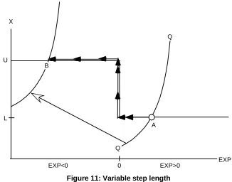
(13) Harrison, Horridge, Pearson and Wittwer. 10. where the RHS is evaluated at H. The effect is that the path jumps back towards X=U, correcting for previously-generated errors.. X H. Q. jump. U. B. jump. L A. Q EXP<0. 0. EXP>0. EXP. Figure 10: Newton corrections. Variable step length to minimize overshooting Normally, each Euler step is of equal length—more precisely, the ordinary change in each exogenous variable is equally apportioned between steps. Before taking such a step it is not hard to compute whether that step will change the state of any complementarity. Indeed, we can modify the length (but not the direction) of the planned step in such a way that at most one complementarity will only just change state. This is illustrated in Figure 11, where, for clarity, Newton correction terms are not shown.. X Q. U. B. L A. Q EXP<0. 0. EXP>0. EXP. Figure 11: Variable step length. The effect of the variable step length is to minimize overshooting. Combining this with the Newton correction described previously, we ensure that that our solution path in the first, approximate,.

(14) A practical method for explicitly modeling quotas and other complementarities. 11. simulation hugs complementarity equations very closely indeed, so enabling our prediction of their final state to be remarkably accurate.. 3.2. Precursors of the latest GEMPACK implementation The approach described in this paper has evolved over a number of years, through several stages: Try-it-and-see closure swapping This approach has been used to simulate import quotas. It is based on Figure 9, but uses the initial state of all complementarities as a first predictor of their final state. We first run a simulation which assumes that all import quotas remain in their current state. Where the quota is binding, we exogenize the import volume and endogenize the corresponding tariff; elsewhere the tariff is exogenous and the import volume adjusts. The results of this first simulation are analysed to see if the post simulation data is consistent with the original assumptions. For example, we would check to see if endogenous import levels were still below quota. If not, the closure (choice of exogenous variables) is adjusted, newly exogenous variables are set to the appropriate levels (eg, import volumes are set to quota values), and the simulation is repeated. The whole process is repeated until the closure and exogenous settings are consistent with the post-simulation data. Past versions of GEMPACK offered no assistance in the necessary processing of simulation results, and consequent adjustment of exogenous settings. All this was laboriously done by hand. In spite of these disadvantages the approach is practical where few complementarities change state, as might be the case in analyzing trade policy with a single-country model. Usually, during simulations of this type, only a small number of quotas either start or stop binding. Where a large number of complementarities both interact and change state, many closure changes will be needed, and the method becomes hopelessly laborious. This might occur, for example in a multi-country model which included many bilateral export and import quotas. In such a case, there is no guarantee that the iterative procedure just described would ever converge. Newton-assisted path following in Euler context Malakellis (2000) constructed a multi-period dynamic CGE model. He used a method akin to Figure 10 to implement non-negativity constraints on investment. A large number of Euler steps had to be used to ensure sufficient accuracy, since there was no second "accurate" simulation. GEMPACK at that time offered no special support for complementarities, so it was necessary to include the complementarity in the model in differential form—leading to model code that was hard to follow. Newton path following in a levels model Horridge et al (1993) constructed a many-period model of water supply and demand which featured many interlocking complementary constraints, derived from constrained optimization problems. The model was specified and solved in the levels, not using GEMPACK, and used a modified Newton approach which incorporated the variable step lengths of Figure 11. Since Newton corrections were applied to every equation, accurate results could be obtained without extrapolation. Using this approach, results could be obtained in minutes or hours which had previously taken days to compute using MINOS (Murtagh and Saunders, 1987). Specialized ancillary programs to automate closure swapping The two-pass method suggested here (approximate simulation to find final state of complementarities, followed by accurate simulation with complementarities omitted) was used by Bach and Pearson (1996) to implement import quotas in the GTAP model. Later Elbehri and Pearson (2000) used similar techniques to treat tariff-rate quotas. Ancillary programs were used to automate the sequence of closure swapping and shock calculation that are needed when quotas change state. Apart from these ancillary programs, no special changes to GEMPACK software were needed. The implementation and explanation were aimed at particular problems (quotas in GTAP) and were not.

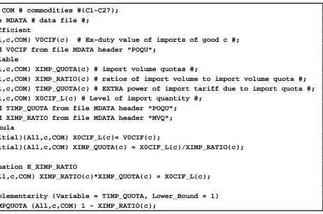
(15) 12. Harrison, Horridge, Pearson and Wittwer. especially transparent to the modeler. Newton corrections (as in Figure 10) were used but not variable step lengths (as in Figure 11). The diagrams used by Elbehri and Pearson to explain tariff rate quotas bore a strong resemblance to Figures 8 and 9. Eventually it was realized that their approach could be generalized to other complementarities. Today: a generalized treatment integral to GEMPACK The approach now implemented in GEMPACK4 refines and extends the Elbehri-Pearson method just described. The new features are: • additions to the TABLO language used by GEMPACK. These allow generalized complementarities to be specified clearly and compactly. • replacement of the Elbehri-Pearson ancillary programs by equivalent routines which are now a standard part of GEMPACK. The new routines require no special setting-up or control by the modeler and issue better diagnostics. • improvement of the Elbehri-Pearson algorithm by using a variable step length to make the initial, approximate simulation more efficient.. 3.3. Specifying a complementarity in GEMPACK Figure 12 contains a fragment of TABLO code5 showing how a complementarity may be set up in GEMPACK. The code implements the import quotas which feature in the simulation described in the next section. The complementarity itself occupies only the last two lines of the excerpt—the preceding lines are background material which we now explain. Set COM # commodities #(C1-C27); File MDATA # data file #; Coefficient (all,c,COM) V0CIF(c) # Ex-duty value of imports of good c #; Read V0CIF from file MDATA header "POQU"; Variable (All,c,COM) XIMP_QUOTA(c) # import volume quotas #; (All,c,COM) XIMP_RATIO(c) # ratios of import volume to import volume quota #; (All,c,COM) TIMP_QUOTA(c) # EXTRA power of import tariff due to import quota #; (All,c,COM) X0CIF_L(c) # Level of import quantity #; Read TIMP_QUOTA from file MDATA header "POQU"; Read XIMP_RATIO from file MDATA header "MVQ"; Formula (Initial)(All,c,COM) X0CIF_L(c)= V0CIF(c); (Initial)(All,c,COM) XIMP_QUOTA(c) = X0CIF_L(c)/XIMP_RATIO(c); Equation E_XIMP_RATIO (All,c,COM) XIMP_RATIO(c)*XIMP_QUOTA(c) = X0CIF_L(c); Complementarity (Variable = TIMP_QUOTA, Lower_Bound = 1) IMPQUOTA (All,c,COM) 1 - XIMP_RATIO(c); Figure 12: A complementarity specified in GEMPACK. 4. GEMPACK Release 8.0, publicly available late 2002, incorporates these features. It is currently in beta test stage.. 5. The example code uses the levels dialect of GEMPACK: the variables and equations are all in the levels..

(16) A practical method for explicitly modeling quotas and other complementarities. 13. The example is of a simple import quota where an implicit tariff, TIMP_QUOTA, is used, if necessary, to restrain import demand to the quota level. In principle, a separate quota may be applied to each commodity—so Figure 12 implements a vector of complementarities indexed over the set COM. V0CIF, the value of imports, is read from file. We take the initial price of imports to be unity (ie, we measure imports in base-period-dollars-worth). This allows us to initially set the volume of imports, X0CIF_L, to equal V0CIF. Two variables are mentioned in the complementarity statement, both of them ratios: • XIMP_RATIO is the actual import volume expressed as a fraction of the quota level; it has an upper bound of 1. • TIMP_QUOTA is the ratio of the user price (inclusive of implicit tariff) to the border (ex-tariff) price; it has a lower bound of 1. Although not required by GEMPACK, the ratio form ensures that both constraint variables have values of the same order of magnitude (around 1). This avoids potential scaling problems—in Figure 8, the 45-degree slope of the dotted lines separating states 1, 2 and 3 presumes that the axis variables are measured on similar scales. The quota complementarity should be in one of two states: (A) quota not binding: XIMP_RATIO<1 and TIMP_QUOTA=1 (B) quota binding: XIMP_RATIO=1 and TIMP_QUOTA>=1 Initial values for both variables are read from file, enabling GEMPACK to check that the complementarity is initially in one of these two states—or post a warning message Since the quota has only two states (binding or not), we can simplify the generalized complementarity: (1) Either X = L and EXP>0 (2) or L<=X<=U and EXP=0 (3) or X=U and EXP < 0. by dropping the upper bound U: (1) Either X = L and EXP>0 (2) or L<=X and EXP=0 To get the GEMPACK statement IMPQUOTA (the name of the complementarity, used to identify it in diagnostic messages): Complementarity (Variable = TIMP_QUOTA, Lower_Bound = 1) IMPQUOTA (All,c,COM) 1 - XIMP_RATIO(c);. we set: X to TIMP_QUOTA L to 1 and EXP to 1 - XIMP_RATIO, so that conditions (1) and (2) above become: (1) Either TIMP_QUOTA = 1 and 1 - XIMP_RATIO>0 (quota not binding) (2) or 1<=TIMP_QUOTA and 1 - XIMP_RATIO=0 (quota binding) which are the same as conditions (A) and (B) above. We could equally set X=XIMP_RATIO (this time with upper bound 1), and so write: Complementarity (Variable = XIMP_RATIO, Upper_Bound = 1) IMPQUOTA (All,c,COM) TIMP_QUOTA(c) - 1;. Indeed we can normally write down two-state complementarities in several different ways. With three-state complementarities we will have less choice, because of an asymmetry: the variable X has two boundary values, L<=X<=U (L and U may be constants or other levels variables) while the expression EXP always has the single "special" value of zero..

(17) 14. Harrison, Horridge, Pearson and Wittwer. Figure 12 omits the code specifying the rest of the model. Amongst much else, the omitted code: • sets the user price of imports to the product of the CIF price and TIMP_QUOTA, • sets demand for imports to be a negative function of the user price, and • assigns the revenues (quota rents) arising from the quota tariff to a model agent (rich households—see below). The first two conditions above ensure that the quota complementarity will have a unique and definite solution (ie, that the R schedule in Figure 3 has positive slope).. 3.4. How GEMPACK treats complementarities during a simulation Apart from adding appropriate statements to the model specification, as shown in Figure 12, the modeler does not need to take any special action to solve models containing complementarities. From the user's viewpoint, simulations are run and results are reported in the normal way. GEMPACK, however, if it detects that a model contains complementarities, sets up and runs the two simulations (first approximate, then accurate) described above. This section provides some details of that process. Each complementarity6 is translated into computer code that evaluates X, L, U, and EXP at the start of every step of a multi-step computation. The evaluations enable the GEMPACK program to determine the state of the complementarity as shown in the first two columns of the table below (see also Figure 8): if X>U+EXP state 3 X=U EXP < 0 else if X<L+EXP state 1 X=L EXP > 0 else state 2 L<X<U EXP = 0 Having established the state of each complementarity, the program then checks if it is true—that is, whether the conditions in the last two columns of the table above do indeed hold. If they do not hold, the solution algorithm must have wandered away from the complementarity—signalling the need for a Newton correction to be applied. For the initial, approximate Euler computation, the program adds to the linearized equation system one of the following three equations for each complementarity, according to its state: if X>U+EXP ∆X + [X-U] = ∆Q state 3 else if X<L+EXP ∆X + [X-L] = ∆Q state 1 else ∆EXP + [EXP] = ∆Q state 2 In the above change equations, the genuine variables are marked by the ∆ symbol. The other terms (in square brackets) are constants evaluated from the values of X, L, U, and EXP at the start of the current step. Notice that if the complementarity was true, the square bracket term for the corresponding state would be zero. Otherwise, the square bracket terms implement the Newton corrections shown in Figure 10. The RHS variable ∆Q is a switch variable created automatically by the system. For each complementarity there is one such variable, which appears only in the associated linear equation. During the initial, approximate computation the ∆Q variables are held exogenously at zero (this switches the equation on). ∆EXP is another "automatic" change variable; one is created by the system for each EXPpression. ∆EXP and ∆X must be endogenous during this first computation. The program's log file will contain a great deal of information about the state and truth of each complementarity at each step of the computation. In particular, it highlights any changes of state. The log also shows when step length has to be shortened to avoid overshooting (see Figure 11).. 6. In the discussion below, we use "complementarity" to refer to individual complementarity conditions. As we saw in Figure 12, a single GEMPACK statement can implement a whole vector (or matrix) of such complementarity conditions..

(18) A practical method for explicitly modeling quotas and other complementarities. 15. At the conclusion of all steps of this first computation a final check is made of the state of every complementarity. This information is used to determine the closure and shocks for the second, accurate, computation, as follows: if X>U+EXP state 3 ∆X will be exogenously shocked so that finally X=U else if X<L+EXP state 1 ∆X will be exogenously shocked so that finally X=L else state 2 ∆EXP will be exogenously shocked so that finally EXP =0 So for each complementarity equation, one previously endogenous variable (∆X or ∆EXP) is made exogenous. To preserve rank, the previously exogenous switch variable ∆Q becomes endogenous, and the equation is switched off. Since each ∆Q appears only in its associated complementarity, endogenizing ∆Q is equivalent to dropping the complementarity condition, leaving only smooth, differentiable equations in the system. With all active equations differentiable we can be sure that a conventional sequence of three Euler (or similar7) computations can be extrapolated to yield an accurate solution. One final check remains. Using results from the extrapolated solution, the software checks that the post-simulation variable values are consistent with the final complementarity states that were predicted by the first, approximate solution, and used to set the closure and shocks for the second, accurate computation. If not, the whole process must be repeated using more, smaller steps in the first, approximate solution, so that it better predicts the final state of all complementarities. Such a repetition of the whole computation is not often needed. By default, GEMPACK chooses a number of steps in the approximate simulation equal to the total number of steps in the second, accurate simulation. If the latter were a 6-8-10 extrapolation, then at least 24 (6+8+10) Euler steps would be used for the first computation. To combat overshooting, some of these 24 steps might have to be divided into two or more parts (as in Figure 11). So perhaps 30 steps would be used. This usually seems to be enough. It adds about 50% to the total solution time that would be needed if the equation system had no complementarities.. 4. Illustration from Indonesia: effects on equity of cutting quota rents The IMF agreed to provide funding to assist in Indonesia’s economic recovery following the 1997 Asian crisis. The IMF required the Indonesian Government to demonstrate a commitment to structural policy reforms. Prior to the crisis, Indonesia’s food imports and exports were regulated by BULOG, a government-sanctioned food trading monopoly. BULOG was restructured as part of the reform process. Its function is now limited to a single commodity, rice, instead of several food types as in the past. An historical objective of BULOG’s operations was to provide cheap rice to the poor. However, the lack of transparency in the past meant that the price of imported rice was much higher for domestic buyers than it would have been under free trade. Considering the administrative burden of such schemes, and the risk, when transfers are involved, of misappropriation, we have reason to fear a poor policy outcome—especially if the administrating body is not publicly accountable. Our assumption is that BULOG’s activities prior to the Asian crisis resulted in restrictions on rice imports. These, at least in earlier years of operation, may not have had a dramatic impact on imports. However, if a quantitative restriction remains in place without an increase in quota as domestic demand grows, then implicit tariffs and the associated quota rents will also rise. That is, policy inertia may result in an ever-growing distortion.. 4.1. The WAYANG model We simulate the effect of lifting rice quotas using WAYANG, a CGE model of Indonesia. WAYANG is a derivative of the Australian ORANI-G model, with some additional features: 7. The Gragg method (a more efficient variant of Euler) would normally be used at this stage..

(19) 16. Harrison, Horridge, Pearson and Wittwer. • •. explicit modeling of import quotas and quota rents, as described in the previous section; an upward-sloping foreign supply schedule for rice imports, reflecting the large size of Indonesia’s potential rice demands compared to the rice surpluses of nearby countries; • a SAM-based mapping of income flows, and • 10 household types, distinguished by income. Each of the 10 households owns factors of production that, together with net transfers from government and foreigners, account for income and income distribution for each household. This feature allows us to turn the new treatment of quota rents into a story of household income distribution. Rather than assume that quota rents are part of government revenue, as we assume for tariff revenues, the model specifies that the wealthiest urban household appropriates quota rents. This means that in addition to the sectoral redistribution effects, we may have a redistribution of income arising from changes in import quotas. In particular, import quotas yield large rents to some richer households. We would expect that removing the quotas should improve income distribution.. 4.2. The simulation We start with a database developed from a 1995 input-output table of Indonesia. In it, imports at basic prices are equivalent to only five per cent of rice sales. We have adapted this database simply by adding the two data vectors required for the new treatment of import quotas. By ascribing (for rice) a value of 1.0 to XIMP_RATIO and 1.7 to TIMP_QUOTA, we assume that implicit in this database, there is a substantial quota rent on rice imports. The value assigned to TIMP_QUOTA is illustrative only, rather than reflecting known estimates of the magnitude of distortion induced by a quantitative restriction on rice imports. The model calculates the value of the rent and distributes it to the wealthiest household in the model. Summary of closure • Aggregate primary factor endowments are fixed. Both types of labour, skilled and unskilled, are perfectly mobile between sectors. However, agricultural industries use no skilled labour. • Agricultural industries use land that is specific to each industry, and capital, which is mobile only within agricultural industries. In non-agricultural industries, fixed capital is specific to each sector. • The balance of trade, aggregate investment and aggregate government expenditure are exogenous. The government’s budget balance is also exogenous.. 4.3. Results Our scenario is to increase the import quota on rice by 10-fold—by shocking XIMP_QUOTA. This alters that state of the quota from binding to non-binding and consequently eliminates the large power of the tax arising from the quota rent. Clearly, removing such a large tax on users is going to induce a sharp decrease in the imported price of rice. Via the assumption of imperfect substitutability, this will induce a smaller decrease in the price of domestically produced rice. The basic price of rice falls by 24.7 per cent for the domestic product, and 50.8 per cent for the imported good. The main reason why the basic import price fall is not larger is because the c.i.f. price rises. The variable pf0cif (i.e., the landed ex-duty import price) increases by 64.0 per cent. This is due to the assumption of a non-zero supply elasticity for rice. TIMP_QUOTA decreases by 70 per cent (from 1.7 down to 1.0), implying that the quota is no longer binding. Prior to the quota increase, rice imports totalled 1514 billion rupiah (of which 1060 billion rupiah was the quota rent) compared with 5389 billion rupiah post-simulation. The volume of rice imports increases by 623 per cent. Given the income distribution feature of this model, we also examine the impact of removing the binding quota on each household. The direct effect is the elimination of the quota rent that the wealthiest urban household received. Yet, in terms of real consumption, this household gains proportionally more than any other from the.

(20) A practical method for explicitly modeling quotas and other complementarities. 17. reform. To explain this, Table 1 contains a decomposition of the contributions to the percentage change in nominal household income (w0hhinc) arising from removing the binding quota. The wealthiest household (“Urban3” in Table 1) loses only 0.77 per cent of initial nominal income through the quota rent being removed. Since “Urban3” owns substantial agricultural land within the database, its returns to land contribute –0.56 per cent to the overall change in nominal income of – 1.59 per cent. For “Urban3”, the fall in CPI of 3.0 per cent more than compensates for the loss in nominal income. Unskilled labour loses from the reform, through the impact of the fall in the price of domestically produced rice on factors used in rice paddy production. Nominal unskilled wages fall by 5.27 per cent, compared with a 0.36 per cent fall for skilled wages. The main reason why “Urban3” does better than other households is because unskilled labour accounts for a smaller proportion of its total income than for any other household (1.3 per cent compared with 47.7 per cent for landless labourers (“Rural1”)). For landless labourers, the contribution of unskilled labour to the overall fall in income is –2.85 per cent, almost equal to its CPI fall of 2.98 per cent. “Rural5”, ostensibly a nonagricultural-based rural household, also loses from the reform because 40 per cent of its income is derived from unskilled labour, which is perfectly mobile between sectors. “Rural3”, “Rural4” and “Rural7” derive more than 7 per cent each of total income from returns to land. Consequently, they suffer significant proportional land income losses due to the reform (-1.41, -1.39 and -1.90 per cent respectively). Only in the case of “Rural4”, among these three households, does the CPI decrease more than compensate for the overall loss in nominal income. Contrary to our a priori reasoning, that removing the quota would improve income distribution, it worsens through the negative effect of the reform on factors that account for a large proportion of the income base of poor households. If we assume that the import supply of rice is infinitely elastic, the losses to “Rural1” and “Rural5” are even larger than before, but all other households gain. This is because the nominal wage of unskilled labour declines even further with removal of the quota, and therefore worsens the outcome for households with a high proportion of unskilled labour in their income base. But other households gain because the further decline in the price of rice also increases the CPI decline, thereby more than compensating for losses in nominal income. Table 1: Real aggregate household consumption. (% change relative to the base case) Rural1 Rural2 Rural3 Rural4 Rural5 Rural6 x3tot_hh -1.042 0.401 -0.237 0.140 -1.425 0.553 w3tot_hh -3.994 -2.592 -3.223 -2.876 -4.350 -2.429 p3tot_hh -2.982 -2.980 -2.992 -3.011 -2.967 -2.966 w0hhinc -3.229 -1.816 -2.452 -2.103 -3.588 -1.653 Decomposition of w0hhinc: rows below add up to row above Land -0.104 -0.222 -1.410 -1.392 -1.001 -0.323 Labour -2.850 -1.587 -0.855 -0.479 -2.412 -0.833 Variable -0.109 -0.209 -0.212 -0.227 -0.105 -0.135 capital Fixed -0.043 -0.001 -0.127 -0.124 -0.095 -0.020 capital Taxes & -0.123 0.203 0.152 0.119 0.025 -0.341 transfers Quota 0 0 0 0 0 0 rents. Rural7 Urban1 -0.137 0.142 -3.156 -2.871 -3.023 -3.009 -2.385 -2.098. Urban2 -0.705 -3.683 -2.999 -2.916. Urban3 0.690 -2.366 -3.035 -1.588. -1.905 -0.370. -0.584 -1.485. -0.376 -2.120. -0.565 -0.171. -0.171. -0.178. -0.079. -0.214. -0.184. -0.043. -0.031. -0.037. 0.245. 0.193. -0.310. 0.168. 0. 0. 0. -0.769.

(21) 18. Harrison, Horridge, Pearson and Wittwer. 5. Conclusion Other algorithms exist for solving problems involving complementarities in economic models, including PATH [see, for example, Dirkse and Ferris (1995)] and MILES (see Rutherford (1993)]. However, those algorithms are designed to solve models which are formulated in the levels. The algorithm presented in this paper does not need explicit levels equations (except for the complementarity itself)—and so can be used in conjunction with initial value solving techniques, such as the Euler method. Furthermore, our approach retains the capacity to extrapolate from several Euler solutions to get a more accurate solution. Extrapolation is needed to make Euler and related methods efficient, and to establish error bounds for results. The new method has been incorporated into the latest version of GEMPACK. All the modeler has to do is add a concise description of each complementarity to the file containing model equations. The software then handles all intricacies of the solution process. The methods described here have been used to model reforms of the European dairy industry - see the report by Berkhout et al (2002). An unavoidable difficulty is that the modeler must formulate each non-negativity constraint or non-differentiable function as a complementarity. This takes a little practice—it would be easy to get a sign wrong, for instance. Such a mistake (or indeed any of the other irritating mistakes which are routinely made during model development) will cause the simulation to go awry. Then begins a painful debugging process. At this too-familiar stage the simplicity of our procedure becomes an advantage. Since the algorithm is easy to understand, and the changing states of each complementarity may be traced through the computations, we may well detect the misplaced sign (say) before too many hours have passed. We hope that this article provides sufficient insight into our algorithm to facilitate such error chasing.. REFERENCES Atkinson, K.E. (1989), An Introduction to Numerical Analysis, 2nd edition, Wiley, New York. Bach, C. and K.R. Pearson (1996), 'Implementing Quotas in GTAP Using GEMPACK or How to Linearize an Inequality', GTAP Technical Paper No. 04, September 1996, pp 37 + 4 Berkhout P., C. van Bruchem, J. Helming and F. van Tongeren (2002), Hervorming EUzuivelbeleid, Den Haag, LEI. Dirkse, S.P. and M.C. Ferris (1995), The PATH Solver: A Non-Monotone Stabilization Scheme for Mixed Complementarity Problems, Optimization Methods and Software, vol. 5, pp. 123-156. Elbehri, A. and K.R.Pearson (2000), 'Implementing Bilateral Tariff Rate Quotas in GTAP using GEMPACK', GTAP Technical Paper No. 18, December 2000, pp. 47+4. Ferris, M.C. and C. Kanzow (2000), Complementarity and Related Problems: A Survey, in P.M. Pardalos and M.G.C. Resende (ed), Handbook of Applied Optimization, (forthcoming), Oxford University Press. Harrison, W.J. and K.R. Pearson (1996), 'Computing Solutions for Large General Equilibrium Models Using GEMPACK', Computational Economics, vol. 9, pp.83-127. [A preliminary version was Impact Preliminary Working Paper No. IP-64, Monash University, Clayton (June 1994), pp.55.] Horridge, M., P. Dixon and M. Rimmer (1993), Water Pricing and Investment in Melbourne: General Equilibrium Analysis with Uncertain Stream Flow, IMPACT Preliminary Working Paper No. IP-63, December 1993, downloadable from http://www.monash.edu.au/policy/elecpapr/ip63.htm Malakellis, M. (2000), Integrated Macro-Micro Modelling under Rational Expectations, PhysicaVerlag, Heidelberg, ISBN 3-7908-1274-9.

(22) A practical method for explicitly modeling quotas and other complementarities. 19. Murtagh, B.A. and M.A. Saunders (1987), ’MINOS 5.1 User’s Guide’, Technical Report SOL 8320R, Dept. of Operations Research, Stanford University, December 1983, rev. Jan. 87. Pearson K.R. (1991), ’Solving Nonlinear Economic Models Accurately via a Linear Representation’, Impact Preliminary Working Paper No. IP-55, Melbourne (July), pp.39. Press, W.H., B.P. Flannery, S.A. Teukolsky and W.T. Vetterling (1986), Numerical Recipes: The Art of Scientific Computing, Cambridge University Press, Cambridge. Rutherford, T. (1993), ’MILES: A Mixed Inequality and Nonlinear Equation Solver’, Working Paper 93-20, Department of Economics, University of Colorado..

(23)

No results found