*
Corresponding author: [email protected]
Validation of numerical methods for flow patterns modeling
based on comparison with the results of laboratory experiments
using visualization methods
Daniil Sergeev1,2*, Alexander Kandaurov1,2, Olga Ermakova1 and Anatoly Suvorov 1
1
Institute of applied physics RAS, Geophysical Research Division, 603950 Ulyanova st. 46, Nizhny Novgorod, Russia
2
Nizhny Novgorod State Technical University n.a. R.E. Alekseev, 603950 Minina st. 24, Nizhny Novgorod, Russia
Abstract. A series of laboratory and numerical experiments were carried out to study the structure of the turbulent flow over a rectangular obstacle for high Reynolds number. The results of numerical simulation performed within ANSYS CFX were verified on data obtained in the wind tunnel of IAP RAS by visualization methods including Particle Image Velocimetry. It was found that the airflow over the obstacle can be conditionally divided into main several regions: the region of the initiation of the detachment and formation shielding zone, the region of the maximum vertical separation and vortex development and the region of flow reattachment. Comparison of numerical calculations with the results of experiments showed that the physical processes of the airflow around model objects can be optimally modeled in a three-dimensional setting using the Detached Eddy turbulence model (DES) with central numerical differentiation scheme and allowed to select optimal parameters of calculation grid.
1 Introduction
Numerical simulation methods are widely used in modern studies of hydrodynamics including turbulent flows. There are two main approaches to the simulation of turbulent pulsations - the direct modeling of spatial and temporal fluctuations of the flows on the base of numerical methods (SRS - Scale Resolve Simulation) [1] and approximate simulation of these fluctuations on the basis of correlation theories and solutions of the Reynolds-averaged Navier-Stokes equations (RANS - Reynolds-Averaged Navier-Stokes) [2]. In the first approach various models of turbulence within DNS (Direct Numerical Simulation), LES (Large Eddy Simulation), ZLES (Zonal Large Eddy Simulation), WMLES (Wall-modeled Large Eddy Simulation), DES (Detached Eddy Simulation), SAS (Scale Adaptive Simulation) [3] may be used. Hybrid methods are often used to overcome the difficulties of using SRS methods related to the problems of robust calculating near solid surface. For example methods based on combining RANS and LES approaches. A classic example of such hybridization is the DES turbulence model [4] - [6].
Calculations made within various numerical schemes demonstrate that the leading role in the formation of the hydrodynamic flow is played by the processes of interaction of turbulent vortices and the boundary layer over solid surface. Numerical models are claimed to accurately reproduce the non-stationary processes of detachment and reattachment of the boundary layer. Flows with a similar behavior (containing separation regions, vortex structures of different scales, and
boundary layers) are often formed behind bodies with poorly streamlined shapes (obstacles, recesses with sharp angles). As a classic example, here we can give a rectangular obstacle. It should be noted that investigations of this type of flow are characterized difficulties in the choice of a numerical scheme that correctly simulates a given flow, as well as in the choice of the parameters of calculating grid. At the same time within the procedure of selecting the number of grid cells, it is often necessary to seek a compromise between the quality of the flow picture reproduction and the adequate time of calculate processing. Thus for the most cases a satisfactory description of flow characteristics requires preliminary Validation of the numerical approaches basing on a comparison with specially performed laboratory experiments.
The most representative method is the validation basing on comparison with flow field picture which could demonstrate qualitative (images) and quantitative (velocity fields) information. The use of laser-optical methods for visualization of the flows made it possible to solve the problem of obtaining a spatial-temporal evolution of the flow. The most modern in this area is Particle Image Velocimetry (PIV). The PIV method is based on the use of laser illumination to visualize particle tracers (seeded in a liquid or gas) and to capture the resulting images on digital video cameras [7], [8]. The advantage of the PIV method over usual contact measurement approaches is that it provides sufficient spatial resolution for large areas of viewing and does not induce perturbations in the flow.
There are many papers devoted to purely experimental investigations of flow around obstacles of various shapes (including poorly streamlined): flows in cavities and near sharp angle surfaces, performed over a wide range of Reynolds numbers [9] - [13]. They mainly use various modifications of PIV-methods. In addition to experimental studies of the features of turbulent flow around bodies of various geometries, numerical simulation of such flows were performed using DNS, LES and DES models [5], [14-20]. It should be noted that the parameters of the coordinate grids (step, overall) often differ greatly between experimental and numerical studies. So it becomes difficult to compare correctly the results obtained in different investigations. Now there is a very small number of works with simultaneous numerical calculations and experiment specially performed to verify them [21-23]. In [21] numerical modeling of the flow around a rectangular obstacle was carried out together with subsequent validation using the PIV method but these results were obtained for low values of Reynolds numbers 269 – 475 corresponding laminar flows. In [22], [23], the Reynolds numbers had values of about 104 but experiments were performed for the flow around the cylinders.
Also it should be mentioned a practical aspect of development methods of validation numerical simulations on the experimental data. Experimental validation of the flows widely used in different applied applications including such important as hydrodynamic processes in power facilities including nuclear plants (see. [24, 25]). To optimize resources for investigations preliminary tests on benchmarks (which could be flows over model objects) are necessary.
This work is purposed to fill the gaps mentioned above. It offers a step-by-step complex approach to validation of numerical calculations on the basis of comparison with the results of a laboratory experiment. The first part of the article is devoted to the description of the methodology of experiments and features of the PIV-methods using for qualitative estimations (mean velocity field). The second part describes the numerical modeling methods and some features of their use for modeling. Then results of validation are presented. The work is summarized in conclusion.
2. Experiment and measurements
The experiments were carried out on a closed wind tunnel of the IAP RAS. The working area represents a rectangular section with a square cross-section 320 × 320 mm and length of 1100 mm. A special feature of the experimental setup is the low level of turbulence intensity at the input of the working section less 0.5 %.
A rectangular obstacle with the dimensions of 497 × 315 × 47 mm was chosen for experiment. The transverse dimension is almost equal to the width of the working area, which ensures a two-dimensional flow in the tunnel.
All experiments were carried for constant air velocity of 8 m/s in the inlet of the tunnel, so corresponding
Reynolds number calculated for the height of obstacle was about ~ 5×10⁴.
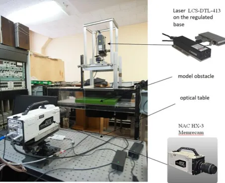
General scheme of experiment is shown on Fig. 1. To obtain a parallel non disturbed flow in front of the obstacle it was placed on a special surface with a well streamlined front edge (thin wing edge).
Fig. 1. The scheme of the obstacle position on the underlying surface with smooth wing edge in the working section of wind tunnel (lighting scheme corresponding the measurements of the overall flow picture).
2.1. Measurements of the flow by visualisation: overall view (qualitative) and velocity fields (quantitative).
The principal scheme for carrying out the PIV measurements was analogous to [26]. The positions of components of PIV in the working section are shown on the photo on Fig. 2. To visualize the flow, solid particles of polyamide (10 μm) were used. Particles were seeded with special injection device installed in expanding-narrowing section before working area. Special test experiments with precise measurements by hotwire demonstrated that injection did not affect on the flow characteristics in the working section. The air flow seeded with particles in the plane along the tunnel was illuminated using a vertical laser sheet (a source was the visible continuous laser with the wavelength of 532 nm, and the power of 1.5 W). The width of the laser sheet was adjusted by a system of cylindrical lenses. The side view was captured by a high-speed camera NAC Memrecam HX-3.
Separate frames of a qualitative picture of all flow structure were analyzed at first. It was necessary to realize the maximum size of the area to be taken by camera for capturing the entire object in the frame. The general scheme of the location laser sheet for this case is shown in Fig. 1. The result of the visualization is shown on Fig. 3 (a).
Instantaneous frames (see Fig. 3) demonstrated: retaining vortex before obstacle (see Fig 3.b), shielding zone (up to 1/3 the length of the obstacle), and the complex dynamics of the vortices of different scales behind it (see Fig 3.a). The vortex sheet is torn from the front ledge of the obstacle. It is carried downstream by the main flow forming a stagnant zone and breaks up into large vortices due to instability and further these vortices decay into chaotic small-scale structures under the action of inertial forces. Then flow again presses to the surface of the obstacle and close the shielding zone.
(a) (b)
Fig. 3 (a) an example of an instantaneous picture of a qualitative flow visualization (size 2560 × 472 pixels, resolution 0.25 pixel /mm, frame rate 2000 frames/second, exposure time 500 μs); (b) an example of a high-resolution visualization of the retaining vortex formed before the obstacle's front ledge (size: 384 × 944 pixels, resolution: 0.166 pixels/mm exposure time 1.25 ms).
We applied the classical cross-correlation image processing for the PIV method in purpose to obtain a quantitative picture of the flow. However the spatial resolution of the obtained overall view (see Fig. 3 a) was clearly not enough to determine the velocity fields at small scales, comparable to the sizes of the observed vortices. Therefore the size camera view and respectively the illumination area were reduced. It was decided to perform measurements in several subsequent cross-sections. In order to obtain a complete average velocity field, nine sections with step 62.5 mm were chosen: the first one above the front ledge, the last - above the back ledge (see Fig. 4). They completely overlap the overall field of observation for the previous case. The overlapping between the sectors in the horizontal direction at the upper surface of the object was 30 mm. The frame rate was increased up to 10000
frames per second. The exposure time of one frame was 20 μs. Successively in each of the sections, the average velocity field was measured. A background was subtracted for each frame before the cross-correlation processing. This allowed to remove the overexposure from the area where the sheet hit the surface which is especially important for capturing image close to the ledge of the obstacle where an intense glare from the wing surface appeared (see Fig 3 b, 5). Two-step adaptive displacement search algorithm was used for cross-correlation analysis when the initial interrogation window 64 × 64 pixel decreased to 32 × 32 pixels (similar to the study [27]). Overlapping of windows was 50%. Thus, the final step of the grid in determining the velocity field was about 2.5 mm.
Fig.4. Scheme of illumination by sectors for obtaining the general velocity field. Distance of 318 and 520 mm indicated vertical sections where velocity profiles were calculated.
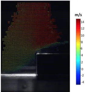
An example of the average velocity field obtained in one section (the first) at the front ledge of the obstacle is shown in Fig. 5. Obtained velocity fields in each sector were linked together (averaged over overlapping regions) to obtain the total average velocity field.
Fig. 5. The image of the front ledge of the body with the airflow velocity field measured by the PIV method (size - 384 × 944 pixels, resolution - 0.166 pixels / mm) exposure time of one frame was 20 μs.
The result of combining average velocity field is shown in Fig. 6. Despite the presence of some empty areas on the average velocity field (low seeding density led to errors), unlike for the instant images (see Fig.3), here it is possible to clearly distinguish the boundaries of the shielding zone of the flow. The maximum error in the PIV measurements at the point was 15 cm/s, and the mean errors was about 2 cm/s.
3 Numerical simulations
The objectives of the studies described in this section were the development of an optimal numerical model for reproducing the flow velocity field observed in the experiment.
Correct modeling of locally unsteady flows of the investigated type in modern computational fluid dynamics is achieved by using special hybrid models of turbulence one of which is the DES model. Its purpose is to combine vortex-resolving models and methods for averaging pulsations in such a way that the flow is modeled by the LES model at a distance from the surface of obstacle and the RANS model is activated in the boundary layer (including the region with strong grid anisotropy).
Within the framework of this model, the Navier-Stokes equations are combined with the equation of incompressibility and equations of transport of the kinetic energy of turbulence k and its dissipation ε with respect to six unknown quantities: the three components of velocity, pressure, and also the quantities k and ε.
Based on the fact that the DES model can only be used to solve the problem in a three-dimensional setting in ANSYS CFX software a three-dimensional model of the flow region was constructed with geometry obtained by redrawing a two-dimensional grid along the transverse axis.
Fig. 7. Side view of the geometry of the simulation area.
For the initial model shown in Fig. 7 the following boundary conditions were first formulated as follows: at the inlet section - a normal flow velocity of 8 m/s was given, at the outlet section - zero pressure; the upper and lower solid surface walls of the wind tunnel - inviscid nonsleep boundary condition , on the surface of the obstacle - viscous sleep condition.
The calculations were performed using a central-difference spatial scheme and an implicit second-order temporal discreet algorithm. The time step of integration was chosen equal to 0.1 ms (equal to time between consequent frames for PIV). This allowed to ensure good
convergence of calculations and correspond (no more than three iterations a time step).
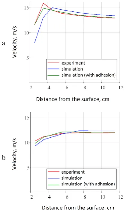
Initially the original three-dimensional model did not take into account viscous boundary and sleep conditions on the lower solid surface above the wing before the ledge. This was done to simplify the construction of an automatic grid and to save computing resources. However the results of calculations showed that the calculated quantitative characteristics of the vortex formation with such simplification differ significantly from the experimental ones near the region of formation of the vortex sheet and separation (the boundary of the shielding zone). An analysis of the results showed that the reason for the differences lies in the incorrect formation of the position of the vortex sheet (the boundary of the shielding zone). This conclusion can be drawn analyzing the figures of the averaged velocity profile in the first section (Fig. 8a). The red curve characterizes the experimental velocity distribution and the blue curve corresponds to the calculation of the initial model in Fig. 8. The reason for this behavior of the average flow was the incorrect flow simulation just before the ledge due to neglect of viscous sleep conditions to the lower surface.
Fig. 8 Time-averaged velocity profiles, calculated from the velocity fields on the first control line in the shielding zone (a) and the second control line in the reattachment zone (b). Positions of control lines are indicated on the Fig. 3.
a
It is seen from Fig. 8 that accepting and applying sleep conditions before the obstacle leads to a significant better agreement with experimental results (the green curve).
Thus, it can be concluded that modeling the dynamics of the boundary layer, not only in the area of intense vortex formation, but also upstream, is an important part of the overall process of high-frequency vortex processes modeling.
Fig. 9. Cell structure of the final three-dimensional numerical model (at the leading edge).
A schematic representation of a grid of the final numerical model (near the front ledge), taking into account the separation of the boundary layer before the ledge is shown in Fig. 9. This model consists of 6 million cells, condensed near the upper leading edge.
The use of more frequent grid near the upper front ledge is performed in order to ensure the correct modeling of high velocity gradients in a vortex sheet coming off the edge and correctly describe the processes of loss the stability of the shear flow. Calculations showed the evolution of the vortex formation in this case is as follows. Near the streamlined front ledge (Figures 10, 11) the vortex sheet is a thin quasi-two-dimensional structure that rapidly loses stability ("collapses" into individual turbulent vortices) which removed downstream. Then, these discrete vortices, due to the inhomogeneous velocity field, lose stability in the direction across the flow and are folded into typical “horseshoe” structures. These initially highly ordered horseshoe vortices are carried downstream, evolving into chaotic structures of different scale. The general picture of the flow, obtained in a numerical experiment, is very close to that observed in the experiment.
Fig. 10. The turbulent flow structure around a model obstacle (velocity contour lines).
The dimensions of the prismatic cells in the shredded region in this case were 0.7 mm, beyond the region of 2.5 mm (similar to the step of the grid in PIV - measurements in the experiment for subsequent comparison). The calculation time on the server of 0.3 TFPS for the final numerical model with the grid shown in Fig. 9, was about a month, taking into account the need to accumulate sufficient statistical information (the length of the simulation realization - 4 s) at a time step of 0.1. Some attempts were made to reduce this time, by reducing the number of cells. However as additional calculations have shown the rejection of a smaller cell near the front ledge results in an increase in the distance from the edge to the point of destruction of the vortex sheet (Fig. 12a) followed by the enlargement of the vortex structures. If the cell size is increased beyond the region up to 3 mm, the structure of the flow becomes quasi-stationary (Fig. 12b).
(a)
(b)
Fig.11. Distribution of the velocity magnitude (a) and vorticity intensity (b) in the central cross-section of the obstacle (instantaneous pictures).
4. Conclusion
in the formation of the hydrodynamic flow. The validation results obtained in the present work showed that the physical processes of flow around model objects can be simulated in a three-dimensional formulation in the best possible way using the DES turbulence model using the central numerical differentiation scheme and optimal parameters of the calculation grid were selected.
This work was partial supported by the Russian Foundation of Basic Research No. 18-48-520023 (providing numerical simulations) and Russian Science Foundation No. 18-19-00473 (providing measurements).
References
1. F.R. Menter, Best Practice: Scale-Resolving Simulations in ANSYS CFD, ANSYS Germany GmbH, 2012. 70 p.
2. C. Fletcher, Computational Techniques for Fluid Dynamics Springer-Verlag Berlin Heidelberg, 1991, 494.
3. I. B. Celik, J. Fluids Eng. 127, 5, 829 (2003). 4. P. R. Spalart, International Journal of Heat and
Fluid Flow. 21, 3, 252 (2000)
5. P. R. Spalart, S. Deck, M. L. Shur, K. D. Squires, M. Kh. Strelets, A. Travin, Theoretical Computational Fluid Dynamics. 20, 181 (2006) 6. A. Travin, M. Shur, M. Strelets, P. Spalart,
Flow, Turbulence and Combustion. 63, 4, 293 (1999)
7. R.J. Adrian Annu. Rev. FluidMech. 23, 261 (1991)
8. R.J. Adrian Experiments in Fluids. 39, 159 (2005)
9. M. K. Shah and M. F. Tachie, Journal of Turbulence. 10, 1( 2009)
10. Y. Z. Liu, F. Ke., H. J. Sung, Journal of Fluids and Structures. 24, 3, 366 (2008)
11. Sherry M., Jacono D. L., Sheridan J. Journal of Wind Engineering & Industrial Aerodynamics. V. 98(12), 888(2010)
12. S.Chun, Y. Z.Liu, H. J. Sung, Experiments in Fluids. 37, 531 (2004)
13. P. K. Panigrahi, A. Schroeder, J. Kompenhans, Experimental Thermal and Fluid Science.
32(4), 1011(2008)
14. M.L. Shur, P.R. Spalart, M.K. Strelets and A.K. Travin, International Journal of Heat and Fluid Flow. 29. P. 1638(2008)
15. Y Egorov, F.R. Menter and D. Cokljat, Journal Flow Turbulence and Combustion. 85(1), 139 (2010)
16. I. I. Vogiatzis, A. C. Denizopoulou, G. K. Ntinas, V. P. Fragos, The Scientific World Journal. 2014, 1 (2014)
17. R. R. Hwang, Y. C Chow, Y. F. Peng, International Journal for Numerical Methods in Fluids. 31 (4), 767(1991)
18. P. K. Panigrahi, S. Acharya, Journal of Fluids and Structures. 20, 2, 235 (2005)
19. M. Breuer, N. Jovicic, M. Kazev, International Journal for Numerical Methods in Fluids. 41, 357(2003)
20. J. Franke, Frank W. J. Wind. Eng. Ind. Aerod.
90, 1191(2002).
21. J.G. Barbosa-Saldaña, O.A. Morales-Contreras, J.A. Jiménez-Bernal, C.C. Gutiérrez-Torres, L.A. Moreno Pacheco, IJRRAS. 15(2), 177(2013)
22. B.S. Dong, G. E. Karniadakis, A. Ekmekci, D. J. Rockwell, Fluid Mech. 569, 185 (2006) 23. P. Parnaudeau, J. Carlier, D. Heitz, E.
Lamballais, Physics of Fluids. 20, 085101, 1(2008)
24. S.M. Dmitriev, D.V. Doronkov, M.A. Legchanov, A.N. Pronin, Solncev, D.N. V.D. Sorokin, A.E. Hrobostov, Thermophysics and Aeromechanics. 23(3), 369(2016)
25. S.M. Dmitriev, A.A. Dobrov, M.A. Legchanov, A.E. Hrobostov, Journal of Engineering Physics and Thermophysics, 88(5), 1297(2015)
26. D.A Sergeev. Instruments and Experimental Techniques. 3, 438 (2009)
27. A.A. Kandaurov, Y.I. Troitskaya, D.A. Sergeev, M.I. Vdovin, G.A. Baidakov. Izvestiya, Atmospheric and Oceanic Physics.