Novel Supervisory Control Algorithm to Improve the Performance of a Real-Time PV Power-Hardware-In-Loop Simulator with Non-RTDS

Article 1

Novel supervisory control algorithm to improve the

performance of a Real-time PV

Loop simulator with non-RTDS

Dae-Jin Kim, Byungki Kim, Hee-Sang Ko, Moon-Seok Jang and Kyung-Sang Ryu* 5

System Convergence Laboratory, Korea Institute of Energy Research, Jeju, South Korea

6

[email protected], [email protected], [email protected], [email protected]

7

* Correspondence: [email protected]; Tel.: +82-64-800-2225

8 9 10

Abstract: A programmable DC power supply with Real-time Digital Simulator (RTDS)-based 11

photovoltaic (PV) Power Hardware-In-the-Loop (PHIL) simulators have been used to improve the 12

control algorithm and reliability of PV Inverter. This paper proposes a supervisory control 13

algorithm for PV PHIL simulator with non-RTDS device that is an alternative solution of high cost 14

PHIL simulator. However, when such a simulator with conventional algorithm which is used in 15

RTDS is connected to a PV inverter, the output is in the transient state and it makes it impossible to 16

evaluate the performance of the PV Inverter. Therefore proposed algorithm controls the voltage and 17

current target values according to the constant voltage (CV) and constant current (CC) modes to 18

overcome the limitation of the Computing Unit, DC power supply and also uses a multi-rate system 19

to account for the characteristics of each component of simulator. A mathematical models of a PV 20

system, programmable DC power supply, isolated DC measurement device and Computing Unit 21

are integrated to form a real-time processing simulator. Performance tests using a PV PHIL 22

simulator which is applied proposed algorithm connected a PV inverter are carried out and proved 23

superiority and utility of this method against conventional methods. 24

Keywords: Photovoltaic; Power-Hardware-In-Loop-Simulator; Supervisory control algorithm; 25

Real-time processing; 26

1. Introduction 27

Photovoltaic (PV) power generation is a technique of converting solar light into electricity. Since 28

the French scientist Edmond Becquerel first discovered the photovoltaic effect in 1839, many 29

advances have been realized for PV power generation, such as the reduced cost and improved 30

efficiency and lifespan of solar cells. This is due to active research and development on the 31

commercialization of solar cells after the oil shock in the 1970s. Because of recent environmental 32

issues and the threat of climate change to the survival of mankind, PV power generation is playing a 33

leading role to meeting the increasing demand for renewable energy. Not only is the distribution of 34

utility-grade PV power plants to replace existing power plants increasing, but small-scale distributed 35

power-grade PV power generators are also gaining prominence. Recently, advances have been made 36

in electric vehicles (EVs) (various related studies have focused on EV charging stations connected to 37

PV power generation), and the percentage of homes combining small PV and EVs that use it as an 38

energy source has been increasing [1–8]. 39

Research is being actively conducted not only on improving the performance of solar power 40

itself (i.e., PV cells, modules, and arrays) but also on peripheral systems to use the generated power. 41

In particular, various studies have been conducted on Maximum Power Point Tracking (MPPT) 42

algorithms to control inverters, which are devices that convert the power generated from a PV, and 43

maximize the output power of a PV system [9-13]. Tests can be performed to apply inverter control 44

algorithm to an actual PV system, but reproducibility is difficult because of changing environmental 45

factors such as the temperature and irradiation. The high cost of implementing actual PV systems to 46

study the improvement of the grid-tied or off-grid PV inverter performance is required in research 47

and development efforts. In order to solve this problem, PV Power Hardware-In-the-Loop (PHIL) 48

simulators, which can simulate and test PV arrays in Real-time, are being used to develop PV 49

inverters [14-17]. PV PHIL simulators are generally composed of universal real-time digital simulator 50

(RTDS) devices, but these are expensive owing to extra features, difficult to use owing to the expertise 51

required to run the program, therefore generally, there is barrier to be widely used. 52

In this paper, a supervisory control algorithm for PV PHIL simulator with non-RTDS is proposed 53

which can improve the output performance developed with a general Computing Unit connected to 54

programmable DC power supply. A multi-rate system is applied to proposed algorithm considering 55

the characteristics of each peripheral devices. A plant consisting of a mathematical model of PV 56

system, control algorithm, calibrations is simulated using the MATLAB/SIMULINK and 57

implemented a form of Real-time processing S/W by means of application program interface API to 58

peripheral components, Real-time Work Shop (RTW), and MEX function. To validate the proposed 59

control algorithm of PV PHIL simulator, an evaluation test is carried out. This included isolated 60

measurement devices for the monitoring output of the DC power supply and digital signal 61

processing of measured signals to interface with peripheral devices. 62

The paper is organized as follows: the next section explains the mathematical modeling of the 63

PV system. Later, in Section 3, presents the proposed control algorithm of PV PHIL simulator against 64

conventional control algorithm and Implementation works such as Real-time S/W, centralized control 65

logic are presented in Section 4. Section 5 presents the simulation and test results validating the 66

performance of the proposed algorithm. Finally, the conclusions close the paper. 67

2. Mathematical Properties of a PV System for the PHIL Simulator 68

2.1. Characteristics of PV Cells for the PHIL Simulator 69

PV cells are the basic components of PV systems. They can be classified by their manufacturing 70

materials as silicon semiconductors or compound semiconductors. In most of the PV industry, PV 71

cells are made of silicon semiconductors with p–n junctions. The mathematical models to predict the 72

electrical properties of PV cells regarding irradiation and temperature are classified as ideal single-73

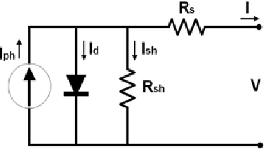
diode, practical single-diode, and two-diode. In this research, the practical single-diode model was 74

used for the PV cell considering the simulator’s real-time computing processing and dynamic model’s 75

accuracy. Figure 1 shows the equivalent circuit [18–20]. 76

77

Figure 1. Equivalent circuit model of PV cell.

78

The output current of a PV cell can be generalized as shown in Equation (1) according to 79

Kirchhoff’s current law (KCL). Electrons and holes appear because of the photoelectric effect caused 80

by light in the depletion layer of p–n semiconductors. The output current appears when a load is 81

connected to both ends and follows the flow of electrons: 82

83

84

where is the photocurrent [A], is the diode current [A], and is the current flowing in the 85

shunt resistance [A]. 86

The output current of this PV cell excludes the current flowing in the diode , and current 87

flowing in the shunt resistance . The output current passes through , and current I is finally 88

output in from the PV cell. If arranged in order, and are as shown in Equation (2): 89

90

= − − 1 − + (2)

91

where is the PV cell output current [A], is the PV cell output voltage [V], is the diode 92

saturation current [A], is the diode abnormal coefficient, is the PV cell series resistance [Ω], and 93

is the PV cell shunt resistance [Ω]. 94

The diode thermal voltage, which is used to find the output current of Equation (2), is 95

determined by the abnormal coefficient value of the non-ideal diode model. This is considered in 96

the following thermal voltage determination formula: 97

98

= (3)

99

where is the diode thermal voltage [V], is the electrical charge of the electron [C], is the 100

Boltzmann constant [J/K], and is the operational temperature [K]. 101

For a PHIL simulator to simulate a voltage-based output current model, Equation (4) is obtained 102

when the PV cell current of Equation (2) is converted into the output voltage. and are 103

dependent on the temperature and are necessary to solve Equation (4); they are determined according 104

to the standard test conditions (STC), as shown in Equations (5) and (6). The bandgap energy E0 varies

105

depending on the type of semiconductor material and temperature. In this research, however, a 106

constant value was used under the assumption of STC. 107

108

= ln 1 + − − (1 + ) −

(4)

= ∙ + ( − ) (5)

= ∙ ( )

[ ( )] (6)

109

Here, is the irradiation under STC, is the temperature under STC, is the temperature 110

coefficient of the photon-induced current [%/C], and is the bandgap energy of the semiconductor 111

[eV]. 112

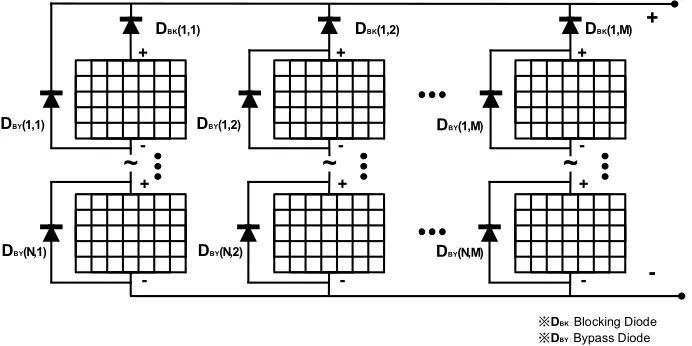
2.2. Characteristics of PV Modules for the PHIL Simulator 113

PV modules are mostly composed of PV cells. The whole PV array is composed of a combination 114

of serial and parallel PV modules depending on the design purpose. The operational voltage is 115

determined by the numbers of serial and parallel PV modules ( , ). Shadows may appear 116

intensity on PV modules may not be the same, which can cause output mismatch inside the modules 118

and lead to problems of deterioration and abrupt power generation decrease. To solve these 119

problems, bypass diodes are used in serially connected PV modules, and blocking diodes are used in 120

parallel PV modules, as shown in Figure 2. 121

DBK(1,1) DBK(1,2)

DBY(N,2)

DBY(1,2)

DBK(1,M)

DBY(N,M)

DBY(1,M)

DBY(N,1)

DBY(1,1)

~

~

~

※DBK : Blocking Diode ※DBY : Bypass Diode

~

+

-+

-+

-+

-+

-+

-+

-122

Figure 2. PV Array integrated with bypass and blocking diode.

123

The bypass diode is connected to the PV module in parallel. In the steady state where the light 124

reaches the PV module homogeneously, the forward bias causes a reverse bias to the bypass diode, 125

and no current flows. However, if an output mismatch between PV modules occurs due to shading, 126

it becomes a reverse bias, which causes a forward bias to the bypass diode. This prevents damage 127

caused by the hotspot phenomenon. The operating formula for the PHIL simulator can be expressed 128

as follows: 129

= − [ − + 1] (7)

where is the voltage drop caused by the bypass diode, is the bypass diode abnormal 130

coefficient, and is the bypass diode reverse saturation current. 131

The PV operating voltage in strings is defined by the number of serial and parallel modules 132

( , ) from Equation (4) and is expressed by the following voltage determination equation: 133

= ln 1 +

− − (1 + )

− (8)

where is the number of PV modules connected in series and is the number of PV modules 134

connected in parallel. 135

Regarding the parallel connection of PV modules, when a voltage imbalance occurs between 136

modules in terms of strings, the output current can flow backwards into the low-voltage module with 137

the shadow due to the voltage mismatch. To prevent this, a blocking diode is installed between 138

modules, and a circuit is composed to prevent current from flowing into the PV module under normal 139

conditions. The module voltage regarding the blocking diode operation can be generalized as follows: 140

= [ + 1] (9)

141

where is the voltage drop caused by the blocking diode and is the bypass diode abnormal 142

The final output of the PV array is the subtraction of the voltage drop used in the 144

parallel connection from the maximum value between and , which refer to the PV module 145

output: 146

= max( , ) − (10)

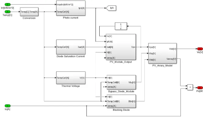
Based on the mathematical model of the PV array including the PV cell, MATLAB/Simulink is 147

used to develop for simulation, as shown in Figure 3. The irradiation and temperature, which are 148

external environment data, and the current value of the PV array are input to output the voltage and 149

current [20]. 150

151

Figure 3. PV System array simulation model.

152

3. Advanced Operation Algorithm of a PV System for the PHIL Simulator 153

3.1. Conventional PV Simulator Operation Algorithm used in RTDS 154

In general, PV simulators that simulate the PV characteristics of invertors or load devices 155

substitute the measured voltage and current values into PV mathematical models and transmit the 156

obtained results to the DC power supply. Figure 4 shows the process of transmitting the generated 157

voltage and current target values to the DC power supply after the input of the initial PV cell 158

parameters PVParams, irradiation Ir(k), temperature Te(k), measured voltage Vm(k), and measured

159

current Im_{(k)into the PV array model [14].}

160

PVParams

Ir(k), Te(k)

Programmable DC Power supply

Block PV Array model

Measurement Block Initial conditions

Vcmd(k), Icmd(k)

Vm_{(k), I}m_(k)

Environment Data

Communication Block

Operation Logic For PV System

161

Figure 4. Conventional PV operation algorithm with RTDS.

However, the combination of general computing unit and typical programmable DC power 163

supply has constraints such as sampling time to peripheral device, computing performance, and 164

rectangular voltage and current output range which are divide into the constant voltage (CV) mode 165

and constant current (CC) mode. One of these modes is activated depending on the load conditions. 166

When a load is connected to the initial DC power supply, the CV mode is started; when the restricted 167

current output range is exceeded, it changes to the CC mode to control the current. The CV mode is 168

then no longer valid, and the output voltage cannot be controlled. Thus, when MPPT control is 169

performed from an inverter, the constant voltage (CV) and constant current (CC) modes cross-170

operate, and the I–V curve of the actual PV system cannot be followed precisely owing to a transient 171

output. 172

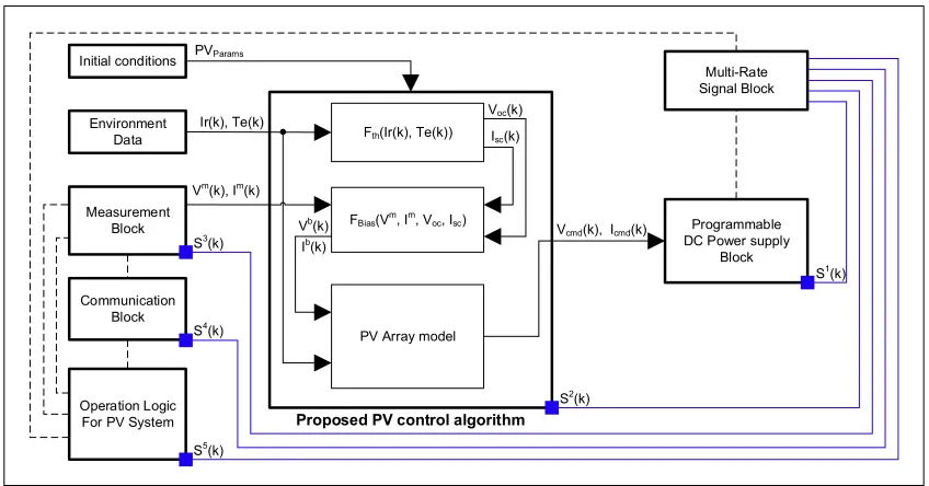
3.2. Proposed Supervisory Control Algorithm for the PV PHIL Simulator with non-RTDS 173

To improve the performance of PV PHIL simulator with non-RTDS connected to grid-tied PV 174

inverter, a supervisory control algorithm and multi-rate system are proposed in this study to 175

optimize the each component responsible for the main functions in Computing Unit, DC power 176

supply, and isolated measurement device. 177

By external environment data to Computing Unit, the PV system characteristic values Voc(k) and

178

Isc(k) are calculated from Fth(Ir(k) and Te(k)), as shown in Equations (11) and (12).

179

= ln 1 + for I = 0 (11)

= ( − − 1 for V = 0 (12)

Vb(k) and Ib(k) are calculated from the function of FBias(Ir, Te, Voc, Isc). Finally, the PV array model

180

results are considered along with Vmod(k), and the reference value (Vcmd(k), Icmd(k)) that will be

181

transmitted to the DC power supply is determined, as shown in Figure 5. The main blocks responsible 182

for the DC power supply control, PV model, measurement devices, communication, and operation 183

control are operated based on the multi-rate system as S1_{(k), S}2_{(k), S}3_{(k), S}4_{(k), and S}5_{(k), respectively.}

184

185

Figure 5. Proposed PV supervisory control algorithm with the multi-rate system.

186

Typical DC power supply start in CV mode, which controls the initial output voltage, and then 187

change to CC mode, which controls the output current when the current limit is exceeded. In CC 188

mode at DC power supply, the output voltage is not controllable due to activation only one mode at 189

a time. 190

Fth(Ir(k), Te(k))

PVParams

Voc(k)

Isc(k)

Ir(k), Te(k)

Programmable DC Power supply

Block FBias(Vm, Im, Voc, Isc)

PV Array model Measurement

Block

Operation Logic For PV System Communication

Block Initial conditions

Vcmd(k), Icmd(k)

Vb_(k)

Vm_{(k), I}m_(k)

Environment Data

Multi-Rate Signal Block

Ib_(k)

S1_(k)

S2_(k)

S3_(k)

S4_(k)

S5_(k)

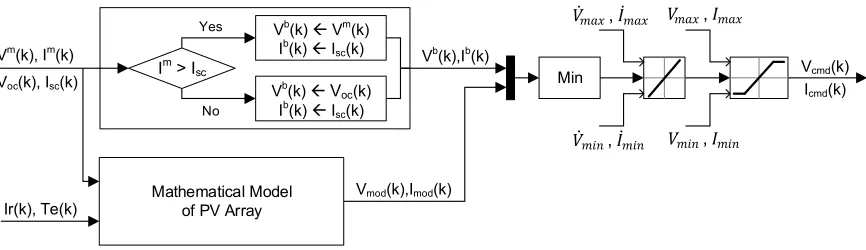
To overcome the limitations of such devices, the proposed control algorithm prevents transient 191

states by comparing the voltage and current outputs in the DC power supply after calculating the I– 192

V value with the maximum voltage Voc and maximum current Isc values according to the current input

193

values of the environment variables. The environmental data Ir(k) and Te(k) for the current step k and

194

the PV system parameters are input, and Equations (11) and (12) are used to calculate the values of 195

Voc(k) and Isc(k). After the DC power supply state are verified, the measurement voltage Vm(k) and

196

current Im_{(k) values being currently output are acquired from the isolated measurement device. The}

197

data are used to calculate Vmod(k) and Imod(k) using the mathematical model of the PV module. The

198

measured output current value and reference current value are compared, and the DC power supply 199

mode is verified. Depending on the mode (CV or CC), the values and ( , ) functions calculated 200

in the above step are used to output Vout(k) and Iout(k). Vcmd(k) and Icmd(k) values can be found through

201

rate limitation and saturation by considering the electrical properties of the PV system and peripheral 202

devices and Figure 6 explains the algorithm in detail. 203

204

205

Figure 6. Proposed control algorithm with limitation values.

206

Because this PV PHIL simulator operates with multiple peripheral devices, it requires efficient 207

control of the characteristics and states of each device. Thus, a multi-rate system that works in 208

accordance with the current state of each device while considering the main control device load was 209

developed. Table 1 presents the function blocks that operate each device and the load weight of each 210

current state. Equation (13) is applied to the standard sample rate ts, and the results of the operating

211

cycle of each device (tDC, tMC, tMU, and tCU) are obtained. Finally, the above results are used to generate

212

the operating signs of S1–5 _{through the pulse generator function PulGen(), as shown in Equation (14).}

213

The cycle of the main block that works in connection with the peripheral devices operates at multiple 214

rates of S1_{(k), S}2_{(k), S}3_{(k), S}4_{(k), and S}5_{(k). The DC power supply transmits and performs the final}

215

reference values of voltage Vcmd(k) and current Icmd(k).

216

Table 1. Load weight of each major function block.

217

Function block Initial stage (IS) System test (ST) Normal operation (NP) Normal stop (NS)

DC power supply (DC)

Main computing unit (MC) Measurement unit (MU) Communication unit (CU) 218 Min Mathematical Model of PV Array Ir(k), Te(k)

Vb_(k),Ib_(k)

Im _{> I} sc

Vmod(k),Imod(k)

Vb_{(k)  V}m_(k)

Ib_{(k)  I} sc(k)

Vb_{(k)  V} oc(k)

Ib_{(k)  I} sc(k)

Yes

No

Vm_{(k), I}m_(k)

Voc(k), Isc(k)

Vcmd(k)

Icmd(k)

,

,

,

= ×

4 × ( ≥ 1) (13)

[ ] = ( [ ] ) (14)

4. Implementation of PV PHIL Simulator 219

4.1. Architecture of the Proposed PV PHIL Simulator 220

A proposed PV PHIL simulator with non-RTDS is composed of DC measurement that can verify 221

the voltage and current values in connection with loads, programmable DC power supply, and 222

Computing Unit which has core functions such as calculation of mathematical model of PV system, 223

communication to peripheral devices, operation, and visualization, as shown in Figure 7. In this 224

system, the Computing Unit and DC power supply interface transmit and receive data through USB 225

communication, and the V–I output value calculated according to the irradiation and temperature 226

data is sent depending on the DC power supply’s current mode. In other words, the voltage and 227

current values measured through serial communication with the analog circuit connected to the load 228

are calibrated and utilized. EtherNET-based TCP/IP communication is performed with peripheral 229

devices for real-time visualization and external environment data. 230

231

232

Figure 7. Architecture and data interface of the proposed PV PHIL.

233

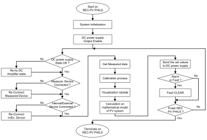
4.2. Integration and conversion to Real-time processing 234

Due to the inputs and outputs are determined from current state of each component, it is 235

necessary to operate PV PHIL simulator systematically. Therefore the centralized control logic is 236

developed to perform the test with certain scenario and is shown in Figure 8, which is described in 237

detail below. 238

Step 1. PV PHILS Initialization procedure: Check the system parameters, UART and TCP/IP communication check, Initialization to the Input and Output

Step 2. Pre-start up procedure: Initial stage to DC power supply and Enable the output power

Step 4. Data processing: Acquisition of the measurement data, calibration process and visualization to the GUI

Step 5. Supervisory control algorithm: Computing the mathematical model of PV system with environmental variables and measured data

Step 6. Execution process: Send the set values to DC power supply and check the fault

Step 7. Repeat the Step 3. ~ Step. 6 until the end of test

239

240

Figure 8. Centralized control logic of the proposed PV PHIL simulator.

241

On the other hand, the software elements including the mathematical model of the PV system 242

mentioned in section 2 should be connected with the hardware and synchronous in Real-time using 243

a general Computing Unit, rather than a special device equipped with an expensive RTDS. An 244

application program interface (API) of programmable DC power supply, MATLAB, Real-time 245

Workshop (RTW), and MEX function are used for code conversion and deployment to Real-time S/W, 246

as shown in Figure 9. 247

248

System Initialization Start on REC-PV PHILS

Measure. Device Connected ?

DC power supply Output Enable

Fault CLEAR Re-try DC

Amplifier state

DC power supply State OK ?

Terminate on REC-PV PHILS

Alarm or Fault ?

Internal/External Device Connected ?

Get Measured data

Calibration process

Calculation on mathematical model

of PV system

Send the set values to DC power supply

Re-Connect Measured Device

Re-Connect In/Ex. Device

Visualization Update Yes

Yes

Yes

No No

No

No

No Finish REC

249

Figure 9. Real-time based PV PHIL Simulator S/W.

250

5. Performance Evaluation of the PV System for the PHIL Simulator 251

To validate the effectiveness of the proposed advanced PV control algorithm and the proposed 252

simulator, an experiment was performed. The proposed method and a conventional method were 253

compared using simulator equipment. The test results were used to compare and analyze the 254

performance characteristics of both methods. 255

5.1. PV Array Simulation and Test Conditions 256

The performance of the proposed algorithm was evaluated with a commercial PV array [21] and 257

Table 2 presents its parameters. The current–voltage characteristics graph of the PV array was 258

calculated with the mathematical model under variable irradiation and temperature conditions and 259

verified. A simulation was performed under two sets of conditions: the irradiation was fixed to 1000 260

W/m2 _{while the temperature varied from 0 °C to 100 °C in 25 °C increments, and the temperature was}

261

fixed to 25 °C while the irradiation was increased from 200 W/m2 _{to 1000 W/m}2 _{in 200 W/m}2

262

increments. 263

Table 2. Specifications of the PV array.

264

Category Value Unit

Model MSX - 60 -

Cell type Polycrystalline silicon -

Maximum power (Pmax) 60 W

Voltage at Pmax (Vmp) 17.1 V

Current at Pmax (Imp) 3.5 A

Open-circuit voltage (Voc) 21.1 V

Short-circuit current (Isc) 3.8 A

Diode quality factor 1.2 -

PV diode band-gap energy 1.124 eV

Number of series cells 36 -

Number of parallel cells 1 -

Number of parallel modules 12 -

Number of parallel modules 1 -

To compare and analyze the performances of the proposed algorithm and the conventional 265

method for a PV PHIL simulator using a DC power supply, a 3 kW PV inverter connected to the 266

system was used. The test was performed at 1000 W/m2 _{and 25 °C. For the current–voltage graph}

considering the PV array’s irradiation and temperature, the operating point was defined with the 268

MPPT control algorithm for the connected inverter. The PV PHILS operating characteristics and 269

performance were compared and analyzed. Tables 3 and 4 present the detailed specifications of the 270

DC power supply and inverter, respectively. 271

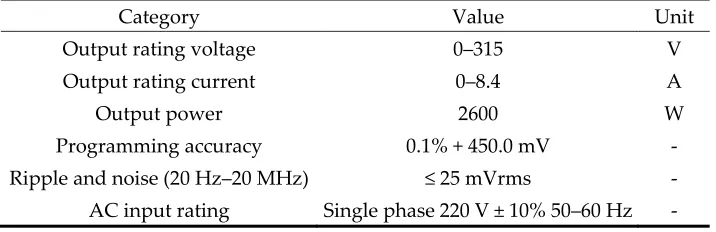
Table 3. Specifications of the programmable DC power supply.

272

Category Value Unit

Output rating voltage 0–315 V

Output rating current 0–8.4 A

Output power 2600 W

Programming accuracy 0.1% + 450.0 mV -

Ripple and noise (20 Hz–20 MHz) ≤ 25 mVrms -

AC input rating Single phase 220 V ± 10% 50–60 Hz -

Table 4. Specifications of the PV inverter.

273

Category Value Unit

Manufacturer DASSTECH -

Model DSP-123K2 -

Max. DC power 3300 W

PV voltage range MPPT 110–450 V

Max. input current 15 A

Nominal AC output 3000 W

AC voltage output 220–240 V

AC connection Single phase -

Max. efficiency 96.7 %

5.2. Simulation Analysis of Performance Characteristics 274

To exactly implement the PV array characteristics according to the irradiation and temperature 275

changes in the PV PHIL simulator, the current–voltage characteristics of the PV array were analyzed 276

in MATLAB with variable external factor conditions. The PV array’s mathematical model and real-277

time operable single-diode PV cell proposed in Section 2 were used. The current–voltage 278

characteristics of the PV array were analyzed while the irradiation and temperature conditions were 279

changed, and the typical current–voltage characteristics proposed by the manufacturer were 280

compared to verify the degree of concordance and accuracy of the results. Figure 10 shows that the 281

voltage–current characteristics of the PV array according to the mathematical model and the voltage 282

and current levels at the maximum current follow-up point proposed by the manufacturer agreed 283

when the temperature was set at 25 °C and the irradiation was incrementally increased from 200 284

W/m2 _{to 1,000 W/m}2_.

286

Figure 10. PV Array I-V Curve with various irradiation.

287

Figure 11 verifies that the voltage–current characteristics of the PV array according to the 288

mathematical model and the voltage and current levels at the maximum current follow-up point 289

proposed by the manufacturer matched when the irradiation was fixed at 1000 W/m2 _{and the}

290

temperature was incrementally increased from 0 °C to 100 °C . Therefore, applying the proposed 291

mathematical model to the PV-PHIL simulator was proven to provide the same characteristics as the 292

operation of an actual PV system. 293

294

Figure 11. PV Array I-V Curve with various temperature.

295

5.3. Experiment Analysis of Performance Characteristics 296

To validate the accuracy of the proposed simulator, Real-time S/W which is included in the 297

mathematical model described in Section 2, the PV control algorithm of the conventional method 298

described in Section 3, and the centralized control logic described in Section 4 is applied to the PV-299

301

Figure 12. Experiment of PV PHIL Simulator with Grid-tied PV Inverter.

302

The initial environment conditions are an irradiation of 1000W/m2 _{and temperature of 25 °C.}

303

No shadow is assumed to appear on any PV module. As shown in Figure 13, with the conventional 304

algorithm of the PV PHIL simulator, the PV array maintained the maximum output voltage Voc state

305

before being connected to the inverter system. However, after connection of the PV inverter to the 306

grid, the voltage and current at the maximum power follow-up point varied continuously and 307

irregularly. 308

309

(a)

311

(b)

312

313

(c)

314

Figure 13. Experiment result with conventional operation algorithm of PV PHILS. (a) I-V Curve characteristic graph of PV System (b) DC power supply voltage output with time series (c) DC power supply current output with time series.

As the PV array output current approached Isc, the I–V curve of the simulation was not followed,

315

and the current–voltage output of the DC power supply was in the transient state. Therefore, in the 316

inverter, the input power varied greatly over time, the MPPT control became unavailable, and the 317

efficiency and performance decreased. In conclusion, when the performance of the PV inverter and 318

MPPT algorithm was evaluated with the PV PHIL simulator using the conventional algorithm, the 319

same characteristics as the actual PV could not be simulated, so a precise evaluation could not be 320

performed. 321

When the proposed advanced operation algorithm was applied to the PV PHIL simulator under 322

the same conditions described above, the initial output characteristics before connection to the PV 323

inverter system revealed the same Voc state as in the case of the conventional algorithm. After

324

connection to the system, the maximum power point tracking was followed. The DC power supply’s 325

output current for the simulated PV array increased with the same pattern as the simulation 326

described in the previous section, as shown in Figure 14. Therefore, with the proposed algorithm, the 327

same characteristics as the actual PV were precisely simulated. Thus, the performance could be 328

330

(a)

331

332

(b)

333

334

(c)

335

To verify the performance of the PHILS algorithm, the Error Current is calculated by the results 336

of each algorithm against the reference values performed through simulation as shown in Equation 337

(15). Reference value of PV output current generated from PHILS is created by () function which 338

has the Look-Up table of PV I-V Characteristic. Figure 15 shows the result of both algorithm and it is 339

clear that the proposed algorithm has much better performance compared to conventional algorithm 340

for PHIL simulator. 341

Error Current(t) = ( ( )) − ( ) (15)

342

Figure 15. Error compared to reference value to each algorithm.

343

6. Conclusions 344

In this research, a supervisory control algorithm for PV PHIL simulators that use programmable 345

DC power supply is proposed as a substitute for existing high-priced RTDS equipment. The 346

effectiveness of this control algorithm was proven by comparison with conventional methods. The 347

main results are summarized as follows. 348

349

(1) The conventional PV algorithm which is used in RTDS equipment was applied to the PV 350

PHIL simulator proposed in this study, but the output is in transient state. However the 351

proposed algorithm confirmed the stable output state with grid-tied PV inverter. In 352

addition, grid-tied PV Inverter was able to perform MPPT control in PV PHIL simulator 353

with the proposed algorithm. 354

(2) A Real-time operating program which is applied to the proposed algorithm, operating 355

control logic, and API functions of peripheral devices was developed and verified the 356

improved performance of the PV PHILS by means of general Computing Unit, DC power 357

supply, and peripherals. 358

(3) With the spreading use of distributed PV power such as household PVs and modular PV 359

containers for isolated areas, the PV PHIL simulator can be used to increase the performance, 360

efficiency, and safety of PV inverters and thus increase competitiveness. 361

362

Acknowledgments:

363

This research was performed in 2017, funded by the Ministry of Trade, Industry and Energy, and supported

364

by the Korean Energy Technology Evaluation and Planning (KETEP) (No. 20172410100030).

365

This work was conducted under the framework of Research and Development Program of the Korea

366

Institute of Energy Research (KIER) (No. B7-2442).

367

Author Contributions: All of the authors contributed to publishing this paper. Dae-Jin Kim carried out

368

modeling, simulations and compiled the manuscript. The literature review and experiments were performed by

Kung-Sang Ryu and Byungki Kim. Hee-Sang Ko and Moon-Seok Jang collected the data and investigated early

370

works.

371

Conflicts of Interest: The authors declare no conflict of interest.

372

References 373

1. Hung, D.Q.; Dong, Z.Y.; Trinh, H. Determining the size of PHEV charging stations powered by commercial

374

grid-integrated PV systems considering reactive power support. Appl. Energy 2016, 183, 160–169.

375

2. Ul-Haq, A.; Cecati, C.; Al-Ammar, E.A. Modeling of a Photovoltaic-Powered Electric Vehicle Charging

376

Station with Vehicle-to-Grid Implementation. Energies2017, 10, 4.

377

3. Khana, O.; Xiaob, W.; Review and qualitative analysis of submodule-level distributed power electronic

378

solutions in PV power systems. Renewable and Sustainable Energy Reviews 2017, 76,516–528

379

4. Zhang, Q.; Tezuka, T.; N. Ishihara, K.; C. Mclellan, B. Integration of PV power into future low-carbon smart

380

electricity systems with EV and HP in Kansai Area, Japan. Renewable Energy 2012, 44, 99–108

381

5. Fathabadi,, H. Novel solar powered electric vehicle charging station with the capability of vehicle-to-grid.

382

Sol. Energy 2017, 142, 136–143.

383

6. Locment, F.; Sechilariu, M.; Forgez, C. Electric Vehicle Charging System with PV Grid-connected

384

Configuration. In Proceedings of the IEEE Vehicle Power and Propulsion Conference (VPPC), Lille, France,

385

1–3 September 2010.

386

7. Birnie, D.P., III. Solar-to-Vehicle (S2V) Systems for Powering Commuters of the Future. J. Power Sources

387

2009,186, 539–542.

388

8. Erickson, L.E.; Robinson, J.; Brase, G.; Cutsor, J. Solar Powered Charging Infrastructure for Electric

389

Vehicles: A Sustainable Development; CRC Press: Boca Raton, FL, USA,2016. 390

9. Xiao, B.; Hang L.;Mei J.,Modular Cascaded H-Bridge Multilevel PV Inverter With Distributed MPPT for

391

Grid-Connected Applications, IEEE Transactions on Industry Applications 2015, 51(2), 1722-1731.

392

10. Moon, S.; Yoon, S.G.; Park, J.H., A New Low-Cost Centralized MPPT Controller System for Multiply

393

Distributed Photovoltaic Power Conditioning Modules, IEEE Transactions on Smart Grid 2015, 6(6) 2649 –

394

2658.

395

11. Karbakhsh, F.; Amiri, M.; Zarchi, H.A., Two-switch flyback inverter employing a current sensorless MPPT

396

and scalar control for low cost solar powered pumps, IET Renewable Power Generation 2017, 11(5), 669-677

397

12. Wang, Y.; Yu, X., Comparison study of MPPT control strategies for double-stage PV

grid-398

connected inverter, Industrial Electronics Society, IECON 2013 - 39th Annual Conference of the IEEE,

399

Vienna, Austria, Nov. 10-13 2013, 1561 - 1565.

400

13. Rout, A.; Samantara, S.; Dash, G. K., Modeling and simulation of hybrid MPPT based standalone PV system

401

with upgraded multilevel inverter, India Conference (INDICON), 2014 Annual IEEE, Pune, India, Dec.

11-402

13 2014, 1-6.

403

14. Nzimako, O.; Wierckx, R., Modeling and Simulation of a Grid-Integrated Photovoltaic System Using a

Real-404

Time Digital Simulator. IEEE Trans. Ind. Applications. 2016, 53(2), 1326–1336.

405

15. Khazaei, J.; Piyasinghe, L.; Miao, Z., Real-time digital simulation modeling of single-phase PV in RT-LAB,

406

PES General Meeting | Conference & Exposition, National Harbor, MD, USA 2014 IEEE, 27-31 July 2014,

407

1-5.

408

16. Mai, X. H.; Kwak, S.K.; Jung, J.H., Comprehensive Electric-Thermal Photovoltaic Modeling for

Power-409

Hardware-in-the-Loop Simulation (PHILS) Applications. IEEE Trans. Ind. Electronics. 2017, 64(8), 6255–

410

6264.

411

17. Mather, B.A.; Kromer, M.A.; Casey, L. Advanced photovoltaic inverter functionality verification using

412

500kw power hardware-in-loop (PHIL) complete system laboratory testing. In Proceedings of the IEEE PES

413

Innovative Smart Grid Technologies (ISGT), Washington DC, USA, February 24–27, 2013.

414

18. Faranda, R.; Leva, S.; Maugeri, V. MPPT techniques for PV systems: Energetic and cost comparison. In

415

Proceedings of the 2008 IEEE Power and Energy Society General Meeting – Conversion and Delivery of

416

Electrical Energy in the 21st Century, Pittsburgh, PA, USA, July 20–24, 2008.

417

19. Desoto, W.; Klein, S.; Beckman, W. Improvement and validation of a model for photovoltaic array

418

performance. Sol. Energy 2006, 80(1), 78–88.

20. Kim,D.J.; Kim, B.K.; Ryu, K.S.; Lee, G.S.; Jang, M.S.; Ko, H.S. Development of PV-power-hardware-in-loop

420

simulator with realtime to improve the performance of the distributed PV inverter. J. Korean Sol. Energy

421

Soc. 2017, 37(3), 47–59.

422

21. SOLAREX MSX-60 and MSX-64 solar panel datasheet. https://www.solarelectricsu pply.com/media/

423

custom/upload/Solarex-MS X64.pdf