Mathematical Model for the Electrokinetic Instability of Electrolyte Flow

(1)

*

Mathematical Model for the Electrokinetic Instability of

Electrolyte Flow

Andrey Shobukhov1,*

1

Lomonosov Moscow State University, F-ty of Computational Mathematics and Cybernetics, Lab for Mathem. Modeling in Physics, RU-119991 Moscow, Russia

Abstract. We study a one-dimensional model of the dilute aqueous solution of KCl in the electric field. Our model is based on a set of Nernst-Planck-Poisson equations and includes the incompressible fluid velocity as a parameter. We demonstrate instability of the linear electric potential variation for the uniform ion distribution and compare analytical results with numerical solutions. The developed model successfully des¬cribes the stability loss of the steady state solution and demon¬strates the emerging of spatially non-uniform distribution of the electric potential. However, this model should be generalized by accounting for the convective movement via the addition of the Navier-Stokes equations in order to substantially extend its application field.

1 Introduction

Electrically induced and controlled electrolyte flows are widely used in various microfluidic systems: pumps, mixers and analyzers. The phenomenon of electrokinetic flow instability, which is often observed in these devices, may limit their performance. But at the same time it can be used in them for mixing the solution components and providing the flow control. Thus understanding of the basic physical processes behind electrokinetic instability becomes very important for further development of microfluidics. But understanding is impossible without proper mathematical modeling. As a result, various boundary problems describing turbulence growth in the laminar electrolyte flow inside the external electric field have been proposed and studied by several research groups worldwide during the last fifteen years.

Zholkovskij, Vorotyntsev et al. consider the problem of modeling the flow in a plane-parallel cell [1] formed by two ion-selective membranes and binary electrolyte solution between them. They propose a system of two continuity equations with respect to the electrochemical potentials of cations and anions coupled with the equa-tions for the stationary creeping incompressible flow. They seek for instability conditions to a certain steady state solution of their model and come to the conclusion that there is a possibility to observe hydrodynamic insta-bility of electrokinetic origin.

Rubinstein, Zaltzman et al. [2-4] study equilibrium electoconvective instability near the charge-selective surfaces. They show that the conclusions from [1] are not quite correct because they imply infinite conductivity of the membranes, which is not the same as perfect charge selection. In [4] they study a 2D system of two Nernst-Planck equations with respect to concentrations of cations and anions, the Poisson equation for the

elec-tric field potential and the Stokes continuity equations for the velocity of the incompressible fluid. Numerical simulations take equilibrium as the initial condition, and static boundary conditions are applied, but the model's response is nonmonotonic both in voltage and in current.

Santiago, Chen et al., unlike previous authors, in a series of papers including [5-7], consider a very long flat channel and demonstrate that high electric field and conductivity gradients may lead to instability. For this setup they develop the Ohmic model of electrolyte solutions which includes the Navier-Stokes equations for incompressible flow. However, they use the Laplace equation for the electric potential, de-facto assuming not only the global electroneutrality of electrolyte, but the local one as well. Basing on it, the authors derive a single conductivity equation instead of the two Nernst-Planck equations for cation and anion concentrations. The authors solve this 2D non-stationary system numeri-cally with various boundary conditions and observe the outbreak and development of oscillations. They study the steady state stability and compare the results of computa-tions and physical experiments.

Demekhin, Shelestov et al. [8] also consider the 2D binary electrolyte flow inside a channel with the electric potential applied to its ends, but they do not assume electroneutrality. They use the Stokes equation for the creeping flow, the Poisson equation for the electric field potential and apply directly the Nernst-Planck equations for the cation and anion concentrations. The equations of the model from [8] practically coincide with those from [4], but the region is different and is much like in [5-7]. The onset of oscillations and the transfer to the chaotic regime is studied both numerically and analytically.

(2)

charged particles distribution. The convection is practically ignored. But the proposed model successfully describes the stability loss of the steady state solution and demonstrates the emerging of spatially non-uniform distribution of the electric potential.

2 Mathematical model

Consider the incompressible viscous flow of electrolyte, which has the density ρ, the velocity U and includes N

types of ions with charges Z1,...,ZN and concentrations

C1,...,CN. Suppose that the flow is driven by the gradient

of pressure P and by the gradient of the electric field potential Φ. Then the flow is described by the Navier-Stokes system of equations combined with N transport equations for densities and the Poisson equation for the electric potential. This general model in whole looks as follows:

(1)

Here F is the Faraday constant, R is the universal gas constant, ε is the dielectric constant, Dj are the diffusion

coefficients of ions and T is the absolute temperature of electrolyte.

In this paper we regard a particular case of (1), which describes the dilute aqueous solution of KCl in the external electric field as a viscous binary electrolyte flow in a long channel with the electric voltage applied to its ends. We suppose that the velocity U and the pressure P are constant. Then the model (1) becomes the Nernst-Planck-Poisson system of equations, which contains the liquid velocity as a parameter:

(2)

In case of the stationary one-dimensional flow in the narrow pipe with the length L0, from (2) we obtain the

equations:

(3)

and supplement them with the boundary conditions:

(4)

We consider only the primary phase of instability right after applying the voltage, when the flow velocity may be still constant. But due to the small initial violation of electroneutrality the instability develops in form of the rapid growth of the electric potential gradient. This is the process we are going to study here.

Following [5], we denote the constants:

(5)

and introduce non-dimensional variables and parameters:

(6)

Here the constant l is the ratio of the longitudinal region size to the transversal one; in the considered one-dimen-sional problem it is just the scaling parameter taken equal to 80. The other values: L0=4·10-2m, Φ0=1·103V,

ε

R=78.3, D1=1·10-9m2/s and D2=2·10-9m2/s, C0=3·10

-2

mol/m3 are taken from [5-7]. The problem (3)-(4) in the dimensionless variables (5)-(6) looks as follows:

(7)

(3)

3 Stability analysis

The problem (7) has the following steady state solution:

(8)

To carry out its stability analysis, we linearize (7) in the vicinity of (8):

(9)

After discarding nonlinear terms we obtain the linear system with respect to small perturbations of c1,c2 and

φ:

(10)

The first two equations of (10) may be solved separately. We search for the concentration perturbations in form of the traveling wave:

(11)

where ω is the complex frequency with the real part ξ and the imaginary part η:

(12)

and k is the real wave number. Having found

c

ˆ

₁and

c

ˆ

₂, we put (11) into the third equation of (10):

(13)

and solve it with respect to

ϕ

~

.

In order to find

c

ˆ

₁and

c

ˆ

₂we substitute (11) into the first two equations of (10) and yield the system of linear algebraic equations with respect to the wave amplitudes:

(14)

Nontrivial solution

(

c

ˆ

₁

,

c

ˆ

₂

)

to this system exists if and only if its determinant equals zero. From this existence condition for the nontrivial solution we get the equations

for the real and imaginary parts of ω. We treat them as the functions of the wave number: ξ=ξ(k) and η=η(k). From (11) it is easy to see: if η(k) >0 then the amplitude of the k-th spatial harmonic exp(ikx) of perturbation grows in time, and thus the solution (8) becomes unstable.

The equations for ξ=ξ(k) and η=η(k), obtained from the solvability condition to (14), look as follows:

(15)

With k=0 the system (15) becomes:

(16)

and its solutions are:

(17)

The values of ξ(0) and η(0) from (17) imply that the spatially uniform perturbation with k=0 is neutrally stable: its amplitude remains constant both over t and over x, and the corresponding solution to (14) satisfies:

(18)

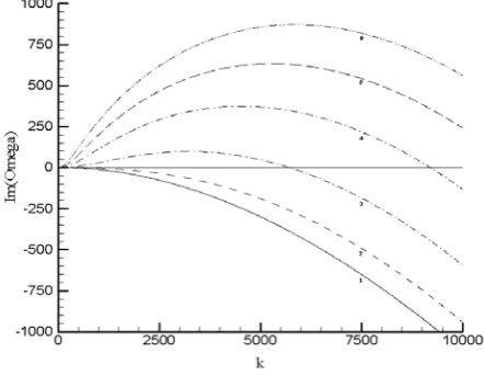
For other values of k we use the parameter continuation method [9]. We suppose that k is continuous and start numerically construct two branches of the curves ξ=ξ(k) and η=η(k) from points A and B. The results obtained for the velocity values 0 ≤ u ≤ 1 are shown in Fig.1.

Fig. 1. Unstable branch A of the curve η=η(k) for different flow velocities: 1: u=0.0; 2: u=0.1; 3: u=0.25; 4: u=0.50; 5: u=0.75; 6: u=1.0.

;

2 ,

1 )),

(

exp(

ˆ

)

,

(

x

t

=

c

⋅

i

kx

−

t

j

=

c

_j _j

ω







=

⋅

+

⋅

=

⋅

+

−

,

0 )

0 (

)

(

)

0 (

)

0 (

2 ,

0 )

0 (

)

(

)

0 (

)

0 (

2 1 2 1 2 2

ξ

α

η

ξ

η

α

ξ

η

(

)

.

)

,

(

;

/

)

(

;

)

,

(

)

,

(

0 2 1

const

u

t

x

u

l

x

l

x

const

c

t

x

c

t

x

c

=

≡

−

⋅

=

≡

=

ϕ

;

Im

Re

ω

ξ

η

ω

=

+

i

⋅

=

+

i

⋅

);

(

~

/

)

(

)

(

);

,

(

~

)

,

(

);

,

(

~

)

,

(

0 2 2 1 1

x

l

x

l

x

t

x

c

t

x

c

t

x

c

t

x

c

ϕ

=

⋅

−

+

=

+

=

.

0 )

(

~

)

0 (

~

);

,

(

~

)

,

0 (

~

);

,

(

~

)

,

0 (

~

).

~

(

~

)

~

(

~

)

(

~

)

~

(

~

)

(

~

2 2 1 1 2 1 0 2 2 2 1 0 2 2 0 2 2 1 1 2 1 0 1 1 0 1 1

=

−

⋅

−

=

−

+

=

−

+

l

t

l

c

t

c

t

l

c

t

c

S

c

S

c

S

Q

c

l

Q

u

c

S

c

S

Q

c

l

Q

u

c

xx xx x t xx x t

ϕ

.

;

2 2 0 2 2 1 1 0 1 1

Q

u

c

S

Q

u

c

S

Q

+

=

+

=

β

α

β

α

(

)

(

)

(

)

ˆ

0 ;

ˆ

;

0 ˆ

ˆ

)

(

)

(

2 2 2 2 2 1 2 2 1 1 1 1 2 1

=

⋅

−

+

⋅

−

=

⋅

−

⋅

−

+

c

k

i

S

k

c

k

i

S

k

ξ

β

η

α

ξ

β

η

α

(

)

(

)

.

0 )

(

)

(

)

(

)

(

2 ;

0 )

(

)

(

)

(

)

(

1 2 2 1 3 2 1 2 1 2 2 1 2 1 4 2 1 1 2 2 1 2 2 1 2 2 1 2 1 2 2

=

+

−

+

−

+

=

+

−

+

−

S

k

S

k

S

k

S

k

S

k

β

η

β

ξ

α

ξη

β

α

η

α

ξ

β

ξ

η

.

0 )

(

)

0 (

Im

)

0 (

,

0 )

0 (

Re

)

0 (

)

;

0 )

0 (

Im

)

0 (

,

0 )

0 (

Re

)

0 (

)

2 1

+

<

−

=

≡

=

≡

=

≡

=

≡

α

ω

η

ω

ξ

ω

η

ω

ξ

B

A

).

0 (

ˆ

)

0 (

ˆ

₂

c

₁

c

=

))

(

exp(

)

ˆ

(

~

2 1

0

c

i

kx

t

S

xx

ω

(4)

In Fig. 1 we show only the branch A of (17), because the branch B produces only negative values of η(k) for all

k>0 with no regard to u, thus it cannot cause instability. Meanwhile the branch A always starts from η(0)=0, and then η(k) either goes directly to negative values (with

u<u*≈0.2, see curves 1-2 in Fig.1) or η(k) first reaches a positive value and only then goes down (with u>u*, see curves 3-6 in Fig.1).

In the former case the solution (7) is neutrally stable, because its perturbation c~1(t,x),c~2(t,x),

ϕ

~(x)has the

spatially uniformal harmonic with k=0, which neither increases nor decreases with time, while all other such harmonics with k>0 decrease. In the latter case the solution (7) is unstable, because its perturbation now contains the growing with time spatial harmonics for those values of k that yield η(k)>0.

4 Numerical results

We apply the results of the stability analysis to further computational investigation of our model. For solving (7) numerically we use the implicit 2-nd order approxi-mation finite difference scheme and solve the resulting equations with the Thomas algorithm. We try different initial distributions of the ion densities and demonstrate that their most important feature is the local electroneutrality:

(19)

Small violation of (19) in the initial density distribution causes the development of the steady state instability.

The initial conditions for c1,c2,

ϕ

are taken from

(8) and are modified by adding small perturbation terms

ϕ

~ , ~ , ~

2 1 c

c . Whatever c~1,~c2,

ϕ

~ we take, the numerical

solution remains constantly equal to (8) if the resulting initial distributions meet the demand (19). But if it is even slightly violated, then the numerical solution leaves the vicinity of (8): see the resulting final distributions of ion concentration and electric potential in Fig. 2 and 3.

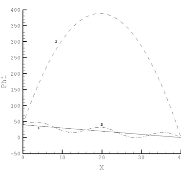
Fig. 2. The final distribution of the cation K+ concentration for different types of perturbations with the flow velocity u=0.25. 1: Electroneutral perturbation; 2: Non-electroneutral constant perturbation; 3: Non-electroneutral sinusoidal perturbation.

Fig. 3. The final distribution of the electric potential for different types of perturbations with the flow velocity u=0.25. 1: Electroneutral perturbation; 2: Non-electroneutral constant perturbation; 3: Non-electroneutral sinusoidal perturbation.

There we demonstrate the final states of solutions to (7) for the following three initial conditions:

(20)

In all these cases the initial electric potential satisfies:

(21)

The curves 1 in Fig.2-3 show that constant and electro-neutral perturbations leave the steady state solution (8) without changes, both for the concentrations and for the potential. The curves 2 in Fig.2-3 show that constant, but not electroneutral perturbation of ion concentrations neither grows nor fades, and may cause increasing of the electric potential inside the flow. Finally, the curves 3 in Fig.2-3 show that the non-electroneutral perturbation of the unstable harmonic (see Fig.1 for k=5, u=0.25) causes the growth of this harmonic both for the concentrations and the potential.

The process demonstrated in Fig.2-3 is not the only way of losing stability in the considered model. Let us study another prototypical transition: evolution in time of a rectangular concentration step. Let the initial data consist of three regions: the left and the right ones – with high ion concentration and the middle – with low ion concentration:

(22)

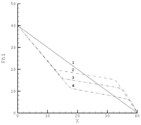
It should be mentioned that the local electroneutrality (19) is strictly observed in (22). Let the electric potential initially satisfy (21). The initial distribution (21)-(22) is shown as curve 1 in Fig.4 and 5.

.

0 ]

,

0 [

)

,

(

)

,

(

₂

1

t

x

=

c

t

x

for

all

x

∈

l

and

t

>

c

.

5 sin

10

0 .

1 )

0 ,

(

,

5 sin

10

0 .

1 )

0 ,

(

:

3 ;

00001

.

1 )

0 ,

(

,

99999

.

0 )

0 ,

(

:

2 ;

99999

.

0 )

0 ,

(

)

0 ,

(

:

1

5 2

5 1

2 1

x

l

x

c

x

l

x

c

x

c

x

c

x

c

x

c

π

⋅

−

=

⋅

+

=

− −

).

/

1 (

)

(

x

=

ϕ

0

⋅

−

x

l

ϕ

.

]

,

4 /

3 [

0 .

1 )

0 ,

(

)

0 ,

(

,

)

4 /

3 ,

4 /

(

5 .

0 )

0 ,

(

)

0 ,

(

,

]

4 /

,

0 [

0 .

1 )

0 ,

(

)

0 ,

(

2 1

l

x

for

x

c

x

c

l

x

for

x

c

x

c

l

x

for

x

c

x

c

∈

=

∈

=

∈

=

(5)

Fig. 3. Unstable branch A of the curve η=η(k) for different flow velocities: 1: u=0.0; 2: u=0.1; 3: u=0.25; 4: u=0.50; 5: u=0.75; 6: u=1.0.

At the same time φ does not keep the initial monotone dependence on x, it quickly forms the regions of rapid increasing and decreasing in the vicinity of electrodes. The formation of these regions with big values of |∂φ/∂x| causes the development of the velocity turbulence at the next stage of the electrokinetic instability.

Fig. 4. The concentrational traveling wave solution of (7) with the initial distribution from (21)-(22); flow velocity u=0.25. 1: t=0, 2: t=5, 3: t=10, 4: t=15.

Fig. 5. The potential traveling wave solution of (7) with the initial distribution from (21)-(22); flow velocity u=0.25. 1: t=0, 2: t=5, 3: t=10, 4: t=15.

Numerical solution for (7) with the initial data (21)-(22) is also shown in Fig.4-5 as curves 2-4. We see that they look like a traveling wave moving right. Such phenomenon for a similar model has been studied back in 1988 [10]. Constant ion concentrations and linear electric potential in the left, right and middle regions, when considered separately, are the steady state solutions to (7), but due to discontinuities of derivatives at x=l/4 and x=3l/4 the initial distribution in whole is not a solution to (7). Never the less, such initial data is smooth enough to produce a classical solution to (7) and is interesting to investigate, because it is a good model of the two-dimensional data sets from [5-7]. We suppose that the observed traveling wave is the first stage of the transition to instability.

The flow velocity u determines the speed of the moving front, and the diffusion slowly blurs the shape of the initial concentration distribution. This is a stable process, which is successfully observed in numerical

experiments. Small perturbations of ion concentrations make approximately the same effect on this traveling wave as they do on the steady state solution: concentra-tion variaconcentra-tions neither fade nor grow, while the electric potential looses monotony. But the model (7)-(8) doesn't take into account the effect of the electric potential on the flow velocity, which is supposed to be constant. For this reason the further development of instability doesn't occur.

5 Conclusion

We have studied a simple one-dimensional model of electrolyte ion movement in the external electric field. The model demonstrates the importance of the local electroneutrality violation for the steady state stability loss and its dependence on the flow velocity.

However, being basically a Nernst-Planck-Poisson system, this model is capable of describing only the first stage of electrokinetic instability: the loss of monotony of the electric potential. Thus for further investigations the model should be enhanced to include convective movement by adding the Navier-Stokes equations.

References

1. E.K. Zholkovskij, M.A. Vorotyntsev, E. Staude, J. Colloid & Interface Science, 181, 28-33 (1996) 2. I.Rubinstein, B. Zaltzman, Physical Review Letters,

114, 114502 (2015)

3. B. Zaltzman, I.Rubinstein, Physical Review Fluids,

2, 093702 (2017)

4. R. Abu-Rjal, N. Leibowitz, S. Park, B. Zaltzman, I. Rubinstein, G. Yossifon, Physical Review Fluids,

4, 084203 (2019)

5. C.-H. Chen, H. Lin, S.K. Lele, J.G. Santiago, J. Fluid Mech., 524, 263-303 (2005)

6. J.D. Posner, J.G. Santiago, J. Fluid Mech., 555, 1-42 (2006)

7. A. Persat, J.G. Santiago, Current Opinion in Colloid & Interface Science, 24, 52-63 (2016)

8. E.A. Demekhin, N.V. Nikitin, V.S. Shelistov, Phys. Fluids, 25, 122001 (2013)

9. M. Kubíček, ACM Transactions on Mathematical Software, 2, 1, 98–107 (1976).