Block Cipher Invariants as Eigenvectors of
Correlation Matrices (Full Version)
?Tim Beyne imec-COSIC, KU Leuven [email protected]
Abstract. A new approach to invariant subspaces and nonlinear invari-ants is developed. This results in both theoretical insights and practical attacks on block ciphers. It is shown that, with minor modifications to some of the round constants, Midori-64 has a nonlinear invariant with 296corresponding weak keys. Furthermore, this invariant corresponds to a linear hull with maximal correlation. By combining the new invariant with integral cryptanalysis, a practical key-recovery attack on 10 rounds of unmodified Midori-64 is obtained. The attack works for 296weak keys
and irrespective of the choice of round constants. The data complexity is 1.25·221 chosen plaintexts and the computational cost is dominated by
256block cipher calls. Finally, it is shown that similar techniques lead to a practical key-recovery attack on MANTIS-4. The full key is recovered using roughly 350 chosen plaintexts and the attack requires about 256
block cipher calls. Furthermore, given less than 350 additional chosen ci-phertexts under a related tweak, 218block cipher calls suffice to recover
the full key.
Keywords: Invariant subspace attack·Nonlinear invariant attack· Lin-ear cryptanalysis·Integral cryptanalysis·Correlation matrices· Midori-64·MANTIS
1
Introduction
Block ciphers are an essential primitive for the construction of many cryptosys-tems. This leads to a natural desire to optimize them with respect to vari-ous application-dependent criteria. Examples include low-latency block ciphers such as PRINCE [7] and MANTIS [5], and the low-power design Midori-64 [3]. Biryukov and Perrin [6] give a broad overview of suchlightweight primitives.
One requirement is shared by all applications: the block cipher must be secure – at the very least it must approximate a pseudorandom permutation. A com-mon design decision that often helps to reduce latency, energy consumption and other cost measures is the simplification of the key-schedule. This, along with other aspects of lightweight designs, has led to the development of new cryptan-alytic tools such asinvariant subspaces[18] andnonlinear invariants [23]. These attacks are the subject of this paper.
?
At CRYPTO 2017, it was shown by Beierle, Canteaut, Leander and Rotella that invariant attacks can often be averted by a careful choice of the round constants [4]. Their work, as well as the earlier work by Todo, Leander and Sasaki on nonlinear invariants [23], invites several questions. This paper will be concerned with three related problems that arise in this context.
1. In their future work sections, Todo et al. [23] and Beierle et al. [4] both express the desire to generalize the nonlinear invariant attack. One can argue that a deeper theoretical understanding of block cipher invariants is helpful, if not essential, to achieve this goal.
2. One potential generalization is the existence of block cipher invariants which are not invariants under all of the round transformations. It is important to investigate this possibility, because such cases are not covered by the techniques introduced by Beierleet al.for choosing the round constants. 3. The previous problem leads to a third question: do such (generalized)
invari-antsonly impact the security of the cipher for a specific choice of the round constants? The results in this paper suggest otherwise.
Contribution. The first of the problems listed above is addressed in Section 4, where the main contribution is Definition 2 and the discussion following it. It is shown that block cipher invariants have an effective description in terms of eigenvectors of correlation matrices. These matrices were first introduced by Daemen, Govaerts and Vandewalle [9] in the context of linear cryptanalysis [21]. As a side result, more insight into the relation between invariants and linear cryptanalysis is obtained.
Section 5 takes a closer look at the invariants of Midori-64, leading up to an example of an invariant of the type described in the second problem above. It will be shown in Section 5.3 that, with minor changes to the round constants, Midori-64 has an invariant which is not invariant under the round function. It applies to 296+ 264 weak keys. Note that this is a significantly larger class of weak keys compared to previous work,i.e.232 for the invariant subspace attack of Guoet al.and 264for the nonlinear invariant attack of Todoet al.[23]. In fact, it will be demonstrated that the invariant discussed in Section 5.3 corresponds to a linear hull with maximal correlation. This observation is of independent interest and will be briefly discussed in Section 5.4.
Section 7 shows that the full key of MANTIS-4 [5] can be recovered given 342 chosen plaintexts. This attack works for all keys provided that a weak tweak is used. The number of weak tweaks is 232(out of 264). The computational cost of this attack is dominated by 256 block cipher calls. If 342 chosen ciphertexts under a related tweak are additionally available, the key can be recovered with a computational cost of 218block cipher calls.
2
Preliminaries and Related Work
Most of the notation used in this paper is standard, for instance (F2,+,·) denotes the field with two elements. Random variables are denoted in boldface.
Many of the results in this work can be compactly described by means of tensor products of real vector spaces. Let V1, . . . , Vn be vector spaces over R. Their tensor product is a real vector spaceV1⊗· · ·⊗Vn. Elements ofV1⊗· · ·⊗Vn
will be called tensors. ForV =V1=· · ·=Vn, the tensor productV1⊗· · ·⊗Vnwill
be denoted byV⊗n. Knowledge of tensor products is not essential to understand
this work.
The invariant subspace attack was introduced by Leander, Abdelraheem, AlKhzaimi and Zenner in the context of thePRINTcipher[18]. LetEk:Fn2 → Fn2 be a block cipher. An affine subspacea+V ofFn2 such that
Ek(a+V) =a+V, (1)
is called an invariant subspace for Ek. The keys k for which (1) holds, will be
called weak keys. At ASIACRYPT 2016, Todo et al. introduced the nonlinear invariant attack as an extension of this attack [23]. A Boolean functionf :Fn
2 → F2 is called a nonlinear invariant for Ek iff there exists a constantc ∈F2 such that for allx∈Fn2,
f(x) +f(Ek(x)) =c.
Importantly, the constantcmay depend on the keyk, but not onx.
The description of block cipher invariants in this paper is based oncorrelation matrices, which were first introduced by Daemenet al.[9]. The definition of these matrices is postponed to Section 3, as they will be introduced from a novel point of view.
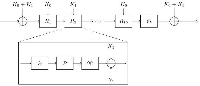
Finally, a brief description of Midori-64 is given here. This information will be used extensively in Sections 5 and 6. Midori-64 is an iterated block cipher with a block size of 64 bits and a key length of 128 bits [3]. It operates on a 64-bit state, which can be represented as a 4×4 array of 4-bitcells. The round function consists of the operations SubCell(S),ShuffleCell (P),MixColumn
(M) and a key addition layer. This structure is shown in Figure 1.
K0+K1
R1
K0
R2
K1
. . . R15 K0
S
K0+K1
S P M
K1
γ2
Fig. 1.The overall structure and round function of Midori-64.
calculations in Sections 6 and 7.
S1(x1, x2, x3, x4) =x1x2x3+x1x3x4+x1x2+x1x3+x3x4+ 1 S2(x1, x2, x3, x4) =x1x2x3+x1x3x4+x2x3x4+x1x4+x1+x4+ 1 S3(x1, x2, x3, x4) =x1x2+x1x4+x2x4+x2+x4
S4(x1, x2, x3, x4) =x1x2x3+x1x3x4+x2x3x4+x1x4+x2x4+x3. The permutationShuffleCell(P) interchanges the cells of the state. It operates on the state as follows:
s1 s5 s9 s13
s2 s6 s10 s14
s3 s7 s11 s15
s4 s8 s12 s16
s1 s15 s10 s8
s11 s5 s4 s14
s6 s12 s13 s3
s16 s2 s7 s9
P
−→
TheMixColumn(M) transformation acts on each state column independently by the following matrix over F24:
M =
0 1 1 1 1 0 1 1 1 1 0 1 1 1 1 0
.
Importantly, round constants are only added to the least significant (rightmost) bit of each cell,i.e.γi∈ {0,1}16.
The tweakable block cipher MANTIS [5] is quite similar to Midori-64, having nearly the same round function. Details will be given in Section 7.
3
Correlation Matrices
The cryptanalysis of symmetric-key primitives is generally based on properties of the plaintext that are reflected by the corresponding ciphertext. To every such property, one could associate a set of values satisfying it. A convenient way to work with sets of plaintexts, or more generally multisets, is to associate a probability space with the set of block cipher inputs. Let x be a random variable on Fn
2 with probability mass function px. The Fourier transformpbx of
pxis defined by
b
px(χu) =
X
x∈Fn2
px(x)χu(x),
whereχu:x7→(−1)u
>x
is a character ofFn2. That is, the functionpxis expressed
in the character basis of the algebra C[Fn2] of functions Fn2 → C. Since the character group ofFn2 is isomorphic toFn2, we may consider pbx to be a function
onFn2 instead. That is,
b
px(u) =E
h
(−1)u>xi,
where E[·] denotes the expected value. Additional information regarding the use of characters and, more generally, representations in the context of proba-bility theory can be found in the references [8, 11].
Example 1. The Fourier transform of the uniform distribution on Fn
2 is zero everywhere except at u= 0, i.e.it has coordinates (1,0, . . . ,0)>. Let p(x) = 0 for allx6=c andp(c) = 1, then bp(u) = (−1)u>c. To stress that
b
pis a vector, we
will regularly use the notationpbu=p(u).b .
The following result is essential to the discussion of the invariants of Midori-64 in Section 5. Note that here, and further on, the vector spaces Fmn
2 and (Fn
2)m are treated as essentially the same. Recall that the symbol “⊗” denotes the tensor product, which in this case coincides with the Kronecker product. Theorem 1 (Independence) Letx1, . . . ,xmbe independent random variables
onFn
2. The Fourier transform of the joint probability mass function ofx1, . . . ,xm
is given by
b
px1,...,xm= m
O
i=1
b
pxi,
Proof. By the independence ofx1, . . . ,xm, we have
b
px1,...,xm(u1, . . . , um) =E
h
(−1)Pmi=1u
> ixii=
m
Y
i=1
Eh(−1)u>ixii.
u t
In fact, Theorem 1 generalizes to arbitrary functions f : (Fn2)m→Csuch that f(x1, . . . xm) =Q
m
i=1fi(xi) withfi∈C[Fn2].
The reader who is familiar with tensors may find it intuitive to consider
b
px1,...,xm in Theorem 1 to be a simple (i.e.rank one) tensor in [R
2n]⊗m. This
fact is not essential to the remainder of the paper.
The discussion so far has been limited to probability distributions. The re-mainder of this section deals with transformations of these distributions. The relation between the probability distribution ofxand F(x) is in general given by a transition matrix. When represented in the basis of characters, such a ma-trix may be called a correlation mama-trix (not to be confused with a mama-trix of second moments).
Definition 1 (Correlation matrix over Fn
2) LetF :Fn2 →Fm2 be a vectorial Boolean function. The correlation matrixCF ∈
R2
m×2n
of F is the representa-tion of the transirepresenta-tion matrix of F with respect to the character basis of C[Fn2] andC[Fm2 ].
Theorem 2 Let F :Fn2 →Fm2 be a vectorial Boolean function with correlation matrixCF. Letxbe a random variable on
Fn2 with probability mass functionpx,
then
b
pF(x)=CFbpx.
Proof. This result is essentially a restatement of Definition 1. ut
It is instructive to consider the coordinates of CF. By the Fourier inversion
formula, we have
px(x) =
1 2n
X
u∈Fn
2
(−1)u>xpbx(u).
By substituting the above into the definition ofpbF(x), and from Theorem 2, one obtains
b
pF(x)(u) =
X
v∈Fn2
1 2n
X
x∈Fn2
(−1)u>F(x)+v>x
bpx(v) =
X
v∈Fn2
Cu,vF pbx(v).
Since this holds for all functionspbx, the coordinates of CF are
Cu,vF = 1 2n
X
x∈Fn2
This establishes the equivalence of Definition 1 and the definition due to Dae-men et al. [9], which originates in the notion of correlation between Boolean functions. Note that (2) coincides with the Walsh-Hadamard transform of F, but since the result of this transformation is not typically interpreted as a linear operator, we will avoid this term.
To conclude this section, a few useful properties of correlation matrices will be listed. These results can also be found (some in a slightly different form) in [9]. In Theorem 5,δdenotes the Kronecker delta function.
Theorem 3 (Composition) Let F : Fl2 → F
m
2 and G : F
m
2 → F
n
2, then CG◦F =CGCF.
Theorem 4 (Orthogonality) Let F : Fn2 → Fn2. If F is a bijection, then its correlation matrix CF is orthogonal.
Theorem 5 (Linear maps) Let L : Fn
2 → Fm2 be a linear map, then Cu,vL =
δ(v+L>u). Furthermore, ifL is bijective,CL is a permutation matrix.
Theorem 6 (Boxed maps) Let F :Fsn
2 →Fsm2 be a vectorial Boolean func-tion such that there exist funcfunc-tions Fi:Fn2 →Fm2 ,i= 1, . . . , s with the property that F = (F1, . . . , Fs). Then
CF =
s
O
i=1 CFi.
In light of Theorem 1, the property expressed by Theorem 6 is intuitively clear: a function satisfying the conditions of Theorem 6 preserves the indepen-dence of its inputs.
Example 2. LetCK denote the correlation matrix corresponding to the function
x7→x+K withx, K ∈F2
2. LetK= (κ1, κ2). By Theorem 6,CK =Cκ1⊗Cκ2. It follows thatCK is given by
CK=
1 0
0 (−1)κ1
⊗
1 0
0 (−1)κ2
=
1 0 0 0
0 (−1)κ2 0 0 0 0 (−1)κ1 0 0 0 0 (−1)κ1+κ2
.
The fact that the correlation matrix of a constant addition is diagonal will be essential to motivate our definition of block cipher invariants in Section 4. .
4
Block Cipher Invariants
cipher, and then to show that this definition includes the nonlinear invariant and invariant subspace attacks as special cases.
Let F : Fn
2 → Fn2 be an arbitrary function – in particular, F need not be bijective. With invariant subspace attacks in mind, it is reasonable to ask which probability distributions are invariant underF. This is equivalent to determining all multisets which are mapped to themselves byF. The solutions to this prob-lem are precisely the eigenvectors of the transition matrix ofF which are also probability distributions. The main issue with this formulation is that, even for a simple function such as the addition of a constant, computing the eigenvectors of the transition matrix is not as trivial as one might hope.
To simplify matters, we will make a change of basis to the character basis of C[Fn2], which was introduced in Section 3. That is, we consider the eigenvectors of correlation matrices instead of transition matrices. This has the important advantage that the correlation matrix of a constant addition is a diagonal matrix. This is helpful, because the columns of a diagonal matrix also form a basis of eigenvectors.
One final simplification can be made before stating Definition 2: there is no good reason to consider only probability distributions – one can simply allow all eigenvectors. It will be shown in Section 4.1 that nonlinear invariants are examples of eigenvectors that are not Fourier transformations of probability distributions.
Definition 2 (Block cipher invariant.) A vectorv∈C2
n
is an invariant for a block cipherEk :Fn2 →Fn2 if it is an eigenvector of the correlation matrixCEk. If v is a multiple of(1,0, . . . ,0)>, it will be called a trivial invariant.
This paper is only concerned with eigenvectors which correspond to real eigenvalues, i.e. ±1 due to Theorem 4. More generally, one could also have eigenvalues which are complex roots of unity. This will be discussed briefly in Section 8, which covers future work.
Not all vectors satisfying Definition 2 can be used in cryptanalysis. A suf-ficient condition for an invariant to be useful is that it depends only on part of the key, and that it comes with an efficient way of testing whether it holds for a given set of plaintext/ciphertext pairs. Section 4.1 shows that the latter requirement is usually not a problem.
Finally, note that some work related to Definition 2 can be found in the liter-ature. Abdelraheemet al.[1] have observed that invariant subspaces correspond to eigenvectors of a submatrix of CEk. This can be seen to be a special case
of Definition 2. Dravieet al. [13] give several results related to the spectrum of correlation matrices (not in the context of invariant attacks).
4.1 Nonlinear Invariants
Theorem 7 (Nonlinear invariant) Let Ek :Fn2 →Fn2 be a block cipher with correlation matrix CEk and f :
Fn2 → F2 a Boolean function with correlation matrix(e0 v)>. If v is an eigenvector of CEk with eigenvalue λ=±1, then for any random variablexon Fn
2, it holds that
Pr [f(Ek(x)) = 0]−
1 2 =λ
Pr [f(x) = 0]−1
2
. (3)
Conversely, suppose(3)holds for a set of random variablesx1, . . . ,xmwith
prob-ability distributions px1, . . . , pxm such thatSpan{px1, . . . , pxm}=R
2n. Then v
is an eigenvector of CEk with eigenvalue λ.
Proof. By the orthogonality of CEk, it holds that CEkv>CEkw = v>w.
Since CEkv =λv withλ =±1, it follows that λv>CEkw =v>wand hence
v>
CEkw=λv>w.
For anyx, choosewas the Fourier transform of the probability mass function of x. The equality v>
CEkw =λv>w is then equivalent to (3). To show the
converse, extract a basis {w1, . . . , w2n} for R2 n
from the vectors pbx1, . . . ,pbxm.
From v>[CEkw
i] = λv>wi, i = 1, . . . ,2n it follows that v>CEk = λv>. The
result follows from the orthogonality ofCEk. ut
Theorem 7 has the following corollary, which gives the precise relation between the eigenvectors ofCEk and the nonlinear invariants ofE
k as defined by Todo,
Leander and Sasaki [23]. Corollary 1 Let Ek :Fn2 →F
n
2 be a block cipher with correlation matrix C
Ek
andf :Fn2 →F2 a Boolean function with correlation matrix(e0 v)>. Thenv is an eigenvector ofCEkwith eigenvalue(−1)c,c∈
F2if and only if for allx∈Fn2, it holds that
f(x) +f(Ek(x)) =c.
Proof. For any x, apply Theorem 7 to a random variable x with probability distribution concentrated on x. For the converse, it suffices to note that the Fourier transforms of these probability distributions form a basis forR2
n
. ut
Finally, the following is a simple result that is useful to obtain the nonlinear invariant corresponding to an eigenvectorv. Note that1S denotes the indicator
function of a setS.
Theorem 8 Let S be any subset of Fn2 and let p1, p2 be functions1 defined by p1(x) = 2−n1S andp2(x) = 2−n1Fn
2\S respectively. Ifv∈F
n
2 is the difference of the Fourier transforms of p1 and p2, i.e., v =pb2−pb1 then 1S has correlation
matrix(e0 v)>.
1
Proof. Clearly, the first row of the correlation matrix of S is given by e>0. For the second row, remark that
vu=
1 2n
X
x∈Fn
2
(−1)1S(x)+u>x= 1
2n
X
x6∈S
(−1)u>x−X
x∈S
(−1)u>x
=bp2(u)−pb1(u).
u t
Example 3. Consider the function F : (x1, x2) 7→ (x2, x1). It has correlation matrix
CF =
1 0 0 0 0 0 1 0 0 1 0 0 0 0 0 1.
.
The vector 2−1(1,1,1,−1)> = 2−2[(3,1,1,−1)>−(1,−1,−1,1)>] is an eigen-vector ofCF. The corresponding nonlinear invariant isf(x1, x2) =x1x2. .
4.2 Computing Invariants
In general, it is nontrivial to compute the invariants of a block cipher. This is in part due to large block sizes, and in part due to the key-dependence of the invariants. To avoid dependencies on the key, one could attempt to find invariants for parts of the block cipher that do not involve the key. The influence of the key addition can easily be checked afterwards. In fact, when working in the character basis, it only depends on the nonzero pattern of the invariant.
The problem is then reduced to computing the invariants of an unkeyed permutationF:Fn2 →Fn2. With Definition 2 in mind, one might consider using a standard numerical procedure to compute the eigenvectors of CF. This is not
a particularly efficient approach: the computational cost is O(23n), which is of
the same order as the ANF-based algorithm proposed by Todoet al.[23] to find nonlinear invariants.
In fact, due to the structure of the matrixCF, its eigendecomposition can
be computed using at most O(n22n) operations. The following algorithm
gen-eralizes the cycle structure approach which is mentioned by Todo et al.[23] as “potentially applicable”. One computes the cycle-decomposition ofF. Then, for each cycle (x0, . . . , xl−1) and for each 0≤j < l, letv(j)be the Fourier transform of the uniform distribution on the singleton {xj}. Letζ =e2π
√
−1/l. For every
0≤k < l, one obtains an eigenvector2 w=Pl−1
j=0ζ
−kjv(j) corresponding to the eigenvalue ζk:
CFw=
l−1
X
j=0
ζ−kjCFv(j)=
l−1
X
j=0
ζ−k(j−1)v(j)=ζkw.
2
This method obtains a complete eigenvector basis, since the sum of all cycle lengths is 2n.
Unfortunately, even the algorithm above is impractical forn = 64. To ob-tain invariants, it is thus necessary to exploit structural properties of the block cipher. Here, Definition 2 will be of use by facilitating a convenient description of invariants. Theorem 9 in Section 5 provides an example in the context of Midori-64.
The main structural property that has been exploited in previous work such as [16, 18, 23] is the existence of non-trivialsimultaneousinvariants for the linear layer and the nonlinear layer of a block cipher. In the first part of Section 5, this approach is briefly revisited from the point of view of Definition 2. Then, more general (i.e. not requiring simultaneous eigenvectors) invariants will be discussed. Note that the discussion in Section 5 will be tailored to the block cipher Midori-64.
5
Invariants for Midori-64
In this section, the invariants of Midori-64 are discussed in the correlation matrix framework. As an example, in Section 5.2 we revisit the invariant subspace attack of Guo et al. [16] and the nonlinear invariant from Todo et al. [23]. Then, in Section 5.3, a more general invariant will be obtained. This invariant will be used in Sections 6 and 7 to obtain practical attacks on (round reduced) Midori-64 and MANTIS.
Before proceeding with the computation of the invariants, it is necessary to analyze the structure of Midori-64 in more detail. Section 5.1 provides the necessary preliminaries.
5.1 State Representation and Round Transformations
In its most general form, the Fourier-domain representation of the Midori-64 state is a vectorv∈C264. Recall from Section 2 that it is convenient to represent the Midori-64 state as a 4×4 array of 4-bit cells. For this reason, we will denote coordinateu= (u1, . . . , u16) with ui ∈F24 ofv byvu =vu1,...,u16. This notation reflects the fact that we can think ofvas a tensor of order 16,i.e.v∈[C24
]⊗16. From Figure 1, and by using Theorem 3, the correlation matrix of the Midori-64 round function is given by
CRi =Cκi+γiCMCPCS,
where κi = K0 when i is odd and K1 when i is even. Recall that Cκi+γi is a diagonal matrix. It follows from Theorem 6 that CS = [CS]⊗16 and CM = [CM]⊗4. The matrixCS ∈R16×16 is a symmetric orthogonal matrix andCM ∈ R2
16×216
is a symmetric permutation matrix. Specifically, we haveCu,vM =δ(u+
M v) by Theorem 5. Finally,CPis a permutation matrix such thatCPv
u1,...,u16 = vuπ−1 (1),...,uπ−1 (16) withπtheShuffleCellpermutation.
3
3
It is convenient to look only for invariants withindependent cellsin the sense of Theorem 1 – but the reader should be reminded that the invariants need not be Fourier transforms of probability distributions. That is, we will assume that there exist vectors v(1), . . . , v(16) such that
vu1,...,u16 = 16
Y
i=1 v(ui)
i. (4)
Equivalently, v = ⊗16
i=1v
(i). Of course, this assumption imposes a serious re-striction. However, assuming (4) greatly simplifies the theory and is sufficiently general to recover the invariant attacks of Guoet al. [16] and Todoet al.[23]. Furthermore, more general assumptions are not necessary to obtain the invariant that will be presented in Section 5.3.
The invariants considered in Section 5.2 will be required to be invariant under S,MandP. Consider the last requirement,i.e.vis an eigenvector ofCP. Recall that CP is a permutation matrix such that
CP 16
O
i=1 v(i)=
16
O
i=1
v(π−1(i)).
Ifv is symmetric, that is,v(1)=· · ·=v(16)=
e
v, then⊗16
i=1v(i)=ve
⊗16is clearly invariant underCP. It turns out that for the purpose of this paper, it suffices to
consider only invariantsv such that there exists someev∈C16 such that
vu1,...,u16 = 16
Y
i=1
e
vui. (5)
That is, v=ev⊗16 and v will be called symmetric, in line with standard termi-nology for such tensors. Note that assumption (5), is less restrictive than (4). Indeed, for any realistic choice of round constants, an asymmetric invariant tends to lead to conflicting requirements on the key after a sufficient number of rounds. Slightly more general invariants can be obtained by requiring thatv(i)is constant on the cycles ofπ.
Computing an eigenvector basis for CS is not difficult. In the remainder
of this section, the eigenvectors of CM satisfying (4) and (5) will be listed. In particular, it is not necessary to compute these eigenvectors numerically. We begin with the straightforward result in Lemma 1. The main result is stated in Theorem 9.
Lemma 1 If v⊗4is a real eigenvector of CM, then there exists a scalarα∈
R0 such that all coordinates ofv in the standard basis are equal to 0or ±α. Proof. The condition thatv⊗4is an eigenvector of CM is equivalent to
v⊗4u
1,u2,u3,u4 =λv ⊗4
Hence, we have for allu1, . . . , u4∈F42 that 4
Y
i=1
vui=λ
4
Y
i=1
vΣj6=iuj. (6)
Note that no vector of the form v⊗4 can correspond toλ=−1, since it follows from (6) that v4u =λvu4. Suppose that at least one coordinate of v is nonzero,
i.e. vu = α for some u. By (6), this implies αv3u0 = α3vu0 for any u0 ∈ F42.
Consequently,vu0 ∈ {0,±α}. ut
Theorem 9 If v⊗4 is a real eigenvector of CM, then A={u | v
u 6= 0} is an
affine subspace of F42 and there exists a scalar α∈R0 such that vu=±αfor all
u∈ A. The converse is also true in the following cases:
– FordimA= 0,dimA= 1anddimA= 2.
– FordimA= 3, provided that the number of negative coordinates ofvis even. The condition for dimA= 3 is also necessary.
Proof. Suppose v⊗4 is a real eigenvector of CM. Let a, u, u0 ∈ F42 such that va 6= 0,va+u6= 0 andva+u0 6= 0. By (6), we have
v2a+u+u0va+u0va+u=v2ava+uva+u0 6= 0.
Hence,va+u+u0 6= 0. It follows thatAis an affine space. Lemma 1 completes the
argument.
To show the converse, first consider the case dimA ∈ {0,1,2}. It suffices to demonstrate that if u1, . . . , u4 ∈ A, then Q
4
i=1vui =
Q4
i=1vΣj6=iuj. Note that {u1, . . . , u4}and{Σi6=1ui, . . . , Σi6=4ui}generate the same affine space. Since the
dimension of this space is at most two, it contains at most four elements. Hence, both products contain the same factors.
For dimA= 3, the previous argument no longer applies whenu1, . . . , u4 are linearly independent. In this case the left and right hand side of Q4
i=1vui =
Q4
i=1vΣj6=iuj involve different variables. Hence, sinceAcontains eight elements,
the products of these elements must be positive. ut
The only symmetric rank one invariants which are not covered by Theorem 9 are those containing only nonzero entries. It would be possible to extend the result to cover this case as well, but this would have little practical value since such eigenvectors can never lead to a significant class of weak keys. This will become clear in Section 5.2.
5.2 Simultaneous Eigenvectors
As discussed in Section 4.2, it is not possible to find the eigenvectors of CEk
of the transformations in the round function. This corresponds to the strategy that is commonly used, and it is the strategy that will be applied in this section. The problem considered in this section is thus to find vectorsv∈R264 such that [CS]⊗16v = λv and [CM]⊗4v = µv with λ, µ ∈ {−1,1}. Furthermore, v must be an eigenvector of CP, but if v is symmetric, we need not separately
consider this requirement. For each of these vectors v, we additionally require that they are eigenvectors of CK+γi for i = 1, . . . ,16. In general, this is not
possible without making some assumptions on the key K.
If {v1, . . . , v16} is a basis of eigenvectors of CS, then the set of all vectors of the form ⊗16
i=1v`i with `i ∈ {1, . . . ,16} is a basis of eigenvectors of [C S]⊗16. Suppose that E+1S is the eigenspace of CS corresponding to eigenvalue 1, and E−1S likewise for eigenvalue−1. Any useful invariant must be an eigenvector of the diagonal matricesCκi+γias well. That is, the invariants must be an element
of one of the vector spaces listed in Table 1.
Table 1.Bases for the intersection of the eigenspaces ofCS andCγi.
∩ Span{e1, e3, . . . , e15} Span{e0, e2, . . . , e16}
ES+1
(1,0,0,0,0,0,0,0,0,0,0,0,0,0,0,0)> (1,0,0,0,0,0,0,0,0,0,0,0,0,0,0,0)> (0,0,1,0,1,0,1,0,−1,0,−1,0,−1,0,−1,0)>
E−S1
(0,1,0,0,0,1,0,0,0,−1,0,0,0,−1,0,−2)> (0,0,0,0,0,0,0,0,0,0,0,0,0,0,0,0)> (0,0,0,1,0,0,0,1,0,0,0,−1,0,0,0,1)>
The vectorsv⊗4should additionally be eigenvectors ofCM. A necessary
con-dition to this end is given by Theorem 9 (in fact, Lemma 1 is sufficient here). Using this result, only four nontrivial invariants of the formv⊗16remain. These are listed in Table 2. The first of these invariants satisfies the conditions of The-orem 8. It corresponds to the nonlinear invariant discovered by Todo, Leander and Sasaki [23]. The eigenvector in the second row of Table 2 corresponds to the invariant subspace obtained by Guoet al.[16].
Table 2.Invariants for Midori-64. Note that the last invariant is simply the nonlinear invariant corresponding to the second invariant (which is an invariant subspace).
Eigenvector (vforv⊗16) Weak-key class Number of weak-keys
(0,0,0,1,0,0,0,1,0,0,0,−1,0,0,0,1)> κ1=κ2= 0 264
(1,0,1,0,1,0,1,0,−1,0,−1,0,−1,0,−1,0)>κ1=κ2=κ3= 0 232
(1,0,−1,0,−1,0,−1,0,1,0,1,0,1,0,1,0)> κ1=κ2=κ3= 0 232
Note that the weak-key class corresponding to a given invariant (the second column in Table 2), is readily determined from the vector v. For instance, con-sider the vector Cκv, with κ= (κ
1, . . . , κ4)> ∈F42 a single nibble of the round key:
v= (0,0,0,1,0,0,0,1,0,0,0,−1,0,0,0,1)>,
Cκv= (−1)κ3+κ4(0,0,0,1,0,0,0,(−1)κ2,0,0,0,(−1)1+κ1,0,0,0,(−1)κ1+κ2)>. Hence,v is invariant underCκ provided that κ
1 =κ2 = 0. Note thatv is also invariant under the addition of the round constants – which has the same effect as modifyingκ4.
An alternative approach to finding invariants starts from the eigenvectors of CM. Theorem 9 makes this method efficient. This will be the starting point to obtain more general invariants in Section 5.3.
5.3 Nonlinear Invariant for “Almost Midori-64”
In the previous section, a few eigenvectors ofCRi were obtained by intersecting
the eigenspaces ofCM, CS andCK+γi. In general the eigenvectors ofCRi are
not eigenvectors of CM or CS. Furthermore, the eigenvectors of CEk need not
be eigenvectors of the round functionsCRi. In order to find all invariants, then,
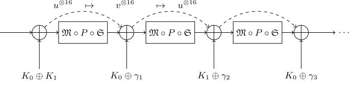
it would be necessary to solve the eigenvalue problem of Definition 2 directly. As discussed before, tackling this problem is out of the scope of this paper, but a slightly more general type of invariant for Midori-64 is presented in this section. Figure 2 shows the general idea: it may be possible to find a vector u⊗16 which is mapped to a vectorv⊗16 byCRi, such thatCRi+1v⊗16=u⊗16. Such a vectoru⊗16 would be an eigenvector ofCRi+1CRi, but not ofCRi.
M◦P◦S M◦P◦S M◦P◦S . . .
K0⊕K1 K0⊕γ1 K1⊕γ2 K0⊕γ3
u⊗16 7→ v⊗16 7→ u⊗16
Fig. 2.Ifu6=v, this figure depicts an invariant for two rounds which is not invariant under one round.
To find such an invariant, it suffices to obtain vectorsu andv =CSusuch that CMu⊗4 =u⊗4 andCMv⊗4 =v⊗4. Theorem 9 provides a complete list of possible choices foruandv. This approach is formalized in Algorithm 14. This
4
algorithm requires a negligible amount of time, as the inner loop is only executed 5216 times – once for each symmetric rank one invariant of CM. Note that it
also returns invariants of the conventional type.
Algorithm 1Finding symmetric rank-one invariants for two rounds of Midori-64.
1: foreach affine subspaceA ⊆F42 withd:= dimA ∈ {0,1,2,3}do
2: S← {1} × {1,−1}2d−2
3: if d= 3then
4: S← {(s1, . . . , s2d−1,
Q
isi)|(s1, . . . , s2d−1)∈S}
5: else
6: S←S× {1,−1}
7: end if
8: for(vu)u∈A∈S do 9: w←CSv 10: A0← {
u∈F42 |wu6= 0}
11: if A0is affineand(dimA06= 3or|{u∈ A0|wu<0}|is even)then
12: yieldv . v⊗16 is invariant for some choice of round constants 13: end if
14: end for 15: end for
A list of invariants produced by Algorithm 1 is given in Appendix A. The most interesting pair of vectorsu, vis given by
u= (0,0,0,0,0,1,0,0,0,0,0,0,0,0,0,0)>
v= (0,0,0,0,0,0,0,0,0,0,−1/2,−1/2,0,0,1/2,−1/2)>.
Clearly,uis invariant under the addition of any constant. Forv, it holds that Cκv= (−1)κ1+κ3/2·(0,0,0,0,0,0,0,0,0,0,−1,(−1)1+κ4,0,0,(−1)κ2,(−1)1+κ2+κ4)>, which is a multiple ofvprovided thatκ2=κ4= 0. For the usual choice of round constants of Midori-64, v is not invariant under the addition of the constants. However, had the round constants been chosen asγi∈ {0,2,8,A}16rather than
γi ∈ {0,1}16, the attack would apply. Moreover, such a restriction only applies
to half of the rounds – the round constants of other rounds may be chosen arbitrarily.
The restriction κ2 = κ4 = 0 (which applies to K0 or K1, but not both) corresponds to a class of 296 weak keys. By Theorem 8,v corresponds to the following nonlinear invariant:
f(x1, . . . , x64) = 16
X
i=1
That is, there exists a constantc∈F2such thatf(Ek(x))+f(x) =cfor allxand
for any even number of rounds. By Theorem 8, ucorresponds to the following “nonlinear” invariant:
g(x1, . . . , x64) = 16
X
i=1
[x4i+x4i−2]. (8)
Hence, for an even number of rounds, g(Ek(x)) +g(x) is constant. Note that
if the number of rounds is odd, the value f(Ek(x)) +g(x) is constant instead.
Appendix B provides test code for this property.
5.4 Trail Clustering in Midori-64
It is worthwhile to take a closer look at the invariantggiven by (8) in Section 5.3. Since g is a linear function, it corresponds to a linear hull with correlation ±1 (where the sign depends on the key). Considering the fact that Midori-64 has been designed with resistance to linear cryptanalysis in mind, this is remarkable. Remark 1 The correlation of any trail in “almost Midori-64” is (much) smaller than2−32, yet there is a linear hull with correlation±1 for296 keys.
The correlation of a linear hull is equal to the sum of the correlations of all trails within the hull. It is well-established that, in theory, this sum could become large even if all terms are small. Such ideas go back to Nyberg [22]. Daemen and Rijmen [10] refer to this effect astrail clustering.
Remark 1 demonstrates an extreme case of trail clustering: the absolute cor-relation of the hull is not just large, it is maximal. This appears to be the first real-world observation of such behavior.
5.5 Additional Weak Keys for the Invariant from Section 5.3
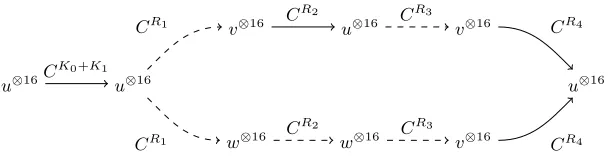
This section shows that the invariantufrom Section 5.3 is invariant under 264 additional weak keys, under the same modifications of the round constants. Al-though 264is small compared to 296, the result is interesting because it provides an example of an invariant over four rounds which is not necessarily invariant over two rounds.
Letu and v be as defined at the end of Section 5.3. For any κ ∈ F4 2 with κ2=κ4= 1, we have
Cκv= (−1)κ1+κ3/2·(0,0,0,0,0,0,0,0,0,0,−1,1,0,0,−1,−1)>. Letw= (−1)κ1+κ3Cκv. By Theorem 9,w⊗4is an invariant ofCM. Furthermore, one can check that wis an eigenvector ofCS.
this. The top branch in Figure 3 corresponds to the discussion in Section 5.3 and holds assuming that K0,4i−2=K0,4i = 1 fori= 1, . . . ,16. The bottom branch
corresponds to a different set of weak keys for whichK0,4i−2 =K0,4i = 1 and
K1,4i−2=K1,4i = 0 fori= 1, . . . ,16. Hence, the 4-round invariant in Figure 3
and its full-round extension hold for 296+ 264 weak keys.
u⊗16 u⊗16
v⊗16 u⊗16 v⊗16
w⊗16 w⊗16 v⊗16
u⊗16 CK0+K1
CR2 CR3
CR2 CR3
CR4
CR4 CR1
CR1
6
Practical Attack on 10 Rounds of Midori-64
The purpose of this section is to demonstrate that the invariant for “almost Midori-64” can be used even when the round constants are not modified. In fact, the attack in this section is valid for any choice of round constants.
Specifically, it will be shown that 10 rounds of Midori-64 are subject to a key-recovery attack that requires 1.25·221chosen plaintexts and has a computational cost of 256 block cipher calls. The downside of this attack is that it is limited to 296 out of 2128 keys. Note that Midori-64 has been analyzed in several prior works. Lin and Wu [19] demonstrate meet-in-the-middle attacks on 10, 11 and 12 rounds of Midori-64. Chen and Wang [24] give a 10 round impossible differential cryptanalysis. The downside of those attacks is that they can not be executed in practice. Table 3 provides an overview of attacks on Midori-64.
Table 3. Overview of key-recovery attacks on Midori-64. Time is measured by the number of encryption operations. Memory is expressed in number of bytes.
Attack Rounds Time Memory Data Weak keys Reference
Meet-in-the-middle 10 299.5 295.7 259.5 N/A Lin and Wu [19] Meet-in-the-middle 11 2122 292.2 253 N/A Lin and Wu [19]
Meet-in-the-middle 12 2125.5 2109 255.5 N/A Lin and Wu [19] Impossible differential 10 280.8 268.1 262.4 N/A Chen and Wang [24]
Invariant subspace 16 216 – 2 232 Guoet al.[16] Nonlinear invariant∗ 16 215h – 33h 264 Todoet al.[23] Integral/invariant 10 256 – 221.3 296 Section 6
∗
This is an attack on a mode of operation. It recovers 32hbits ofhencrypted blocks.
The attack presented below is based on the observation that integral proper-ties [17] and invariants can often be combined. However, since we allow arbitrary round constants in this section, the invariant can only be used once. In this re-gard the nonlinear invariant that was introduced in Section 5.3 has an important advantage: with one assumption on the key, it covers two rounds.
6.1 Nonlinear Property for 6 Rounds of Midori-64
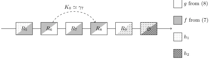
R5 R6 R7 R8 R9 S
K0'γ7
gfrom (8)
f from (7)
h1
h2
Fig. 4.Nonlinear property over six rounds of Midori-64. The notation “'” is used to indicate equality in the second and fourth bits of every nibble of each of its arguments.
The functions h1 and h2 in Figure 4 depend on the choice of the round constants. Specifically,h1depends onP−1(M(γ5+γ7)) andh2depends onγ7+γ9. For the purposes of this paper, a detailed description ofh1is not necessary. For h2, it holds that
h2(x1, . . . , x64) = 16
X
i=1
f(S(x4i−3, x4i−2, x4i−1, x4i) +γ7,i+γ9,i).
In general,hj can be written in the form
hj(x1, . . . , x64) = 16
X
i=1
h(βj,2i,βj,2i+1)(x
4i, x4i+1, x4i+2, x4i+3), (9)
whereβj∈F322 is a constant depending on the round constants. In particular,β2 consists of the second and fourth bits of every nibble ofγ7+γ9. For the default choice of round constants of Midori-64, βj,2i = 0. Hence, only two different
Boolean functions can occur as terms in (9): h(00)(x1, x2, x3, x4) =x2+x4
h(01)(x1, x2, x3, x4) =x2x3x4+x1x3x4+x1x2x3+x1x4+x1+x2. Since the functionsh1andh2are balancedon every cellof the state, it holds that P
x∈Shi(x) = 0 withS a set of state values such that every cell takes all
values exactly once. This makes it possible to combine integral cryptanalysis with the 6-round nonlinear property described above.
6.2 Integral Property for 4 Rounds of Midori-64
“C”. Subscripts are used to denote groups of values which jointly satisfy the “A” property. Note that cells can be part of several groups,e.g.a cell marked “Ai,j”
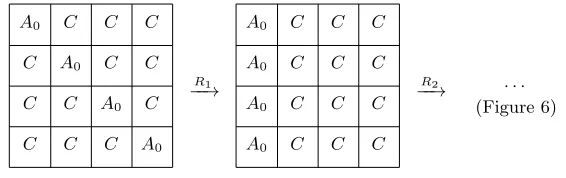
is contained in groups iandj. The Midori-64 designers discuss the existence of a 3.5 round integral distinguisher. In fact, one can see that a 4-round integral property5 exists. Note that the property is nearly identical to the Rijndael dis-tinguisher discussed by Knudsen and Wagner [17], the difference being that the property works better than expected for Midori-64.
A0 C C C
C A0 C C
C C A0 C
C C C A0
A0 C C C
A0 C C C
A0 C C C
A0 C C C
R1
−−→ R2
−−→ · · ·
(Figure 6)
Fig. 5.First two rounds of the integral property for four rounds of Midori-64.
The integral property is based on a set of chosen plaintexts such that the diagonal cells take all possible values exactly once and all other cells are constant. After one round, the same property then holds for the first column whereas all other cells are constant. This is shown in Figure 5.
The effect of the remaining rounds is shown in Figure 6. Figure 6 shows that, before the last application ofM, any four distinct cells in a column jointly satisfy the “A” property. This implies that all cells can be labeled “A” after four rounds.
The derivation in Figure 6 starts by forming appropriate groups of cells which are independent before the third round. Four (sometimes overlapping) groups of such cells are indicated using “Ai”,i = 0, . . . ,3 in Figure 6. The maps S and
P preserve the groups. Furthermore, one can see that four new groups can be obtained after the application ofM. These groups can be chosen in such a way that they are aligned in different columns of the state afterP has been applied. The four round property then follows.
6.3 Combination of the Nonlinear and Integral Properties
The final attack can now be described. Figure 7 provides an overview. Let I
denote a set of plaintext/ciphertext pairs with the structure required by the integral property from Figure 5. Then, due to the nonlinear property from Fig-ure 4, the following holds:
X
(P,C)∈I
h2(C+K0+K1) =
X
(P,C)∈I
h1((R4◦ · · · ◦R1)(P+K0+K1)) = 0. (10)
5
C A1 A A2,3
A0 A2 C A1
A2,3 A0 A3 C
A1 C A A0
C A1 A1 A2
A2 A0 C A0
A3 A3 A2 C
A0 C A3 A1
C A2 A1 A2
A0 A1 C A0
A2 A3 A0 C
A1 C A3 A3
C A2 A3 A1
A0 A1 C A0
A2 A0 A2 C
A3 C A1 A3
C C C C
A3 A1 A1 A1
A2 A A2,3 A2,3
A0 A0 A0 A
C C C C
A2 A1 A0 A0
A0 A3 A2 A3
A1 A2 A3 A1
C C C C
A0 A2 A1 A0
A1 A3 A2 A2
A3 A0 A3 A1
C C C C
A2 A2 A3 A0
A1 A1 A1 A2
A3 A0 A0 A3 ↓P◦S
A0 A1 A A2
A A0 A2 A3
A3 A A0 A1
A2 A3 A1 A
A0 A1 A3 A
A1 A A2 A3
A A2 A0 A1
A2 A3 A A0
A0 A A3 A2
A1 A0 A2 A
A3 A2 A A1
A A3 A1 A0
A A1 A3 A2
A1 A0 A A3
A3 A2 A0 A
A2 A A1 A0 ↓M
A0 A1 A2 A3
A0 A1 A2 A3
A0 A1 A2 A3
A A A A
A0 A1 A2 A3
A0 A1 A2 A3
A A A A
A0 A1 A2 A3
A0 A1 A2 A3
A A A A
A0 A1 A2 A3
A0 A1 A2 A3
A A A A
A0 A1 A2 A3
A0 A1 A2 A3
A0 A1 A2 A3 ↓P◦S
↓M
A A A A
A A A A
A A A A
A A A A
↓M
Hence, every setI defines a low-degree nonlinear polynomial equation in (part of) K0+K1. Given enough such equations, one observes that a Gr¨obner basis for the ideal generated by these polynomials can be efficiently (within a second on a regular computer) computed. Although computing Gr¨obner bases is hard in general, it is easy in this case due to the fact that key bits from different cells are never multiplied together.
Note that only those key bits which are involved inh2in a nonconstant way can be recovered by solving the system of polynomial equations. That is, the number of key bits recovered is four times the number of nonlinear terms in (9). For the default Midori-64 round constants, 40 key bits can be recovered. It was observed that these bits are often uniquely determined given 40 equations. This requires 40·216 = 1.25·221 chosen plaintexts. A more detailed analysis of the data requirements is provided in Section 6.4.
The remaining 24 bits ofK0+K1can be guessed, along with the 32 unknown bits inK0. This requires 256block cipher calls. Note that this additional work is only necessary after it has been established that a weak key is used. Hence, an attacker in the multi-key setting has a very efficient method to identify potential targets.
R1 R2 R3 R4 R5 R6 R7 R8 R9 S
K0'γ7
K0+K1 K0+K1
Integral property
Fig. 7.Overview of the attack on 10 rounds of Midori-64.
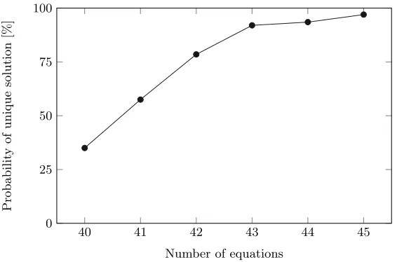
6.4 Detailed Analysis of the Data Requirements
The data requirements of the attack are determined by the number of equations that are necessary to recover the 40 bits of K0+K1 that can occur as indeter-minates in (10). If the constant cells of each integral plaintext set are selected independently and uniformly at random, then the probability that the system of equations has a unique solution may be computed. Figure 8 provides an estimate of this probability based on a sample of 200 key-recovery experiments.
For 40 equations – i.e. 1.25·221 chosen plaintexts – Figure 8 shows that the probability of recovering all 40 bits of the key is roughly 35%. With one additional equation, a probability of nearly 60% is obtained.
40 41 42 43 44 45 0
25 50 75 100
Number of equations
Probabilit
y
of
unique
solution
[%]
Fig. 8.Probability that the system of equations for key-recovery has a unique solution. The equations are constructed from (10) by selecting the constant cells in the integral plaintext sets independently and uniformly at random.
7
Practical Attack on MANTIS-4
This section presents an attack on the block cipher MANTIS [5], which is closely related to Midori-64. Dobraunig, Eichlseder, Kales and Mendel give a practical attack against MANTIS-5 in the chosen tweak setting [12]. This attack has been extended to six rounds by Eichlseder and Kales [14]. The attack presented in this section is limited to MANTIS-4, but the assumptions about the capabilities of the attacker are different. The attacker is not allowed to choose the tweak, but it is assumed that a weak tweak is used. It will be shown that for every choice of the key, there are 232 (out of 264) weak tweaks. When a weak tweak is used, the full key can be recovered from (on average) 346 chosen plaintexts and with a computational cost of approximately 256block cipher calls. If, in addition, 346 chosen plaintexts for a single related tweak are available, the computational cost reduces to roughly 218block cipher calls. Table 4 contains an overview of attacks on MANTIS.
Table 4. Overview of key-recovery attacks on MANTIS–r. Time is measured by the number of encryption operations.
Attack r Time Memory Data Weak tweaks Reference
Truncated differential∗ 5 228 – 238 N/A Dobrauniget al.[12]
Truncated differential∗ 6 253.5 – 253.5 N/A Eichlsederet al.[14] Zero-correlation/integral∗†3/7 266.2 248.4 253.7 N/A Ankeleet al.[2] Integral/invariant 4 256 – 346 296 Section 7.1 Integral/invariant∗ 4 218 – 692 296 Section 7.4
∗These attacks rely on related tweaks. †
This attack applies to a version of MANTIS with an asymmetric number of rounds in the inbound (3) and outbound (7) direction. Such attacks are not considered in this paper, but the techniques from this section could be used to obtain key-recovery attacks for MANTIS-6/4.
Figure 9 illustrates the overall structure of MANTIS-4. Unlike in Midori-64, the round key K1 is the same in all rounds. Additional whitening keysK0 and K00 = (K0 ≫ 1) + (K0 63) are added before the first round and after the last round. The round function is nearly identical to the Midori-64 round function, the difference being that the round keys and constants are added before rather than after the application ofM. Hence, the 2-round nonlinear invariant for Midori-64 also applies to MANTIS-4. Note that the values of the round constants RC1, . . . ,RC4 are not essential to the attack described here.
enables extending the 6-round nonlinear property of Midori-64 to eight rounds. The presence of a tweak allows mounting a weak tweak rather than a weak key attack, which corresponds to a significantly weaker adversarial model.
R1 R2 R3 R4 S
M
S R−41
R−31 R−21
R−11
σ σ σ
σ T
K1 K1 K1 K1
α+K1
α+K1
α+K1
α+K1
K00+K1+T+α
K0+K1+T
Fig. 9.Overview of MANTIS-4.
7.1 Description of the Attack
An overview of the attack is shown in Figure 10. As in the attack on Midori-64 from Section 6, a few initial rounds are covered by an integral property. Since the nonlinear property extends over eight rounds for MANTIS, it suffices to use a weaker integral property. Figure 11 shows the property that will be used. It requires 16 chosen plaintexts.
The nonlinear property is similar to the property that was discussed in Sec-tion 6, but slightly more complicated. Specifically, due to the tweak-key schedule, the functions h1 and h2 can depend on the tweak. As for Midori-64, h1 and h2 can be written in the form
hj(x1, . . . , x64) = 16
X
i=1
h(βj,2i,βj,2i+1)(x
4i, x4i+1, x4i+2, x4i+3), (11) where βj = (βj,1, . . . , βj,32) ∈ F322 is a constant that possibly depends on the tweak and the functionsh(βj,2i,βj,2i+1) are given by
h(00)(x1, x2, x3, x4) =x2+x4
h(11)(x1, x2, x3, x4) =x2x4+x1+x2+x3
h(01)(x1, x2, x3, x4) =x2x3x4+x1x3x4+x1x2x3+x1x4+x1+x2
R1 R2 R3 R4 S
M
S R−41
R−31 R−21
R−11
σ σ σ
σ
gfrom (8)
f from (7)
h1
h2
T
K1 K1 K1 K1
α+K1
α+K1
α+K1
α+K1
K00 +K1+T+α
K0+K1+T
α+K1+σ3(T)'RC3
Integral property
Fig. 10. Nonlinear property over eight rounds of MANTIS-4. The notation “'” is used to indicate equality in the second and fourth bits of every nibble of each of its arguments.
Note that all of these functions are balanced. The constant β1 consists of the second and fourth bits of every nibble ofα. For convenience, this will be denoted byβ1'α. Forβ2, we haveβ2'RC1+α+K1+σ(T). This implies that
β2'RC1+ RC3+σ(T) +σ3(T).
LetIdenote a set of plaintext/ciphertext pairs such that the plaintexts have the structure required by the integral property, then
X
(P,C)∈I
h2(C+K00 +K1+T+α) =
X
(P,C)∈I
h1(R1(R2(P+K0+K1+T))) = 0.
A C C C
C C C C
C C C C
C C C C
C C C C
A C C C
A C C C
A C C C
R1
−−→
C A A A
C A C A
C A A C
C C A A
R2
−−→
Hence, each set I corresponds to a low-degree polynomial equation in (part of) the key. As in Section 6, a Gr¨obner basis for the ideal generated by these polynomials can be efficiently computed.
As in the attack on Midori-64, only those key bits which are involved in h2 in a nonconstant way can be recovered by solving the system of polynomial equations. For simplicity, assume that the functionsh(00), h(01),h(10) andh(11) all occur as terms in (11) in the same proportion. Then the expected number of key bits that can be recovered by solving the system of polynomial equations is equal to 40.6 For obtaining 40 key bits, it was observed that 40 equations are sufficient. This requires 24·40 = 640 chosen plaintexts.
The remaining bits of the whitening keyK00 +K1 (24 bits on average) can then be guessed, along with the 32 unknown bits of K1. For each such guess, it is possible to compute K00 (since K00 +K1 is already known) and hence K0. No additional plaintext/ciphertext pairs are necessary to carry out this process. Hence, the work required for the entire key-recovery attack is then roughly 256 block cipher calls.
7.2 Reducing the Data Requirements by Overlapping Integral Sets
Figure 11 shows one possible integral property for two rounds of MANTIS, but many alternatives exist. One example is shown in Figure 12. Since the input sets for the integral properties in Figures 11 and 12 overlap for an equal choice of the constant cells, the data requirements can be reduced.
For example, to obtain 40 distinct integral sets from only 316 chosen plain-texts, one proceeds as follows. First, choose 28plaintexts such that the first byte of the state takes all possible values. This yields a total of 32 overlapping integral sets of size 16: half of these correspond to the integral property in Figure 11, the other half to that in Figure 12. For the eight remaining integral sets, choose one of the already queried plaintexts and build the integral set by letting the third cell take all possible values – this corresponds to yet another integral property similar to that in Figures 11 and 12. Overall, this requires 28+ 8·15 = 316 chosen plaintexts.
Note that the same technique can be applied to the attack on Midori-64 from Section 6, but it only reduces the data requirements by 40 chosen plaintexts.
7.3 Detailed Analysis of the Data Requirements
As remarked in Section 7.1, the number of whitening key bits that may be recovered depends on the value of the tweak. Specifically, it depends on the value ofβ2 in (11). Recall thatβ2 consists of the second and forth bits of each nibble of RC1+ RC3+σ(T) +σ3(T). Indeed, every term of the form h(01) or h(10) may contribute four unknowns to the system of equations in the key. A
6
C A C C
C C C C
C C C C
C C C C
C A C C
C C C C
C A C C
C A C C
R1
−−→
C A A C
C C A A
C A A A
C A C A
R2
−−→
Fig. 12.Alternative integral property for two rounds of MANTIS.
term of the formh(11)contributes at most two unknown key bits, whereash(00) is linear and hence does not supply any key bits.
In Section 7.1, it was estimated that 40 bits of the key may be recovered. This corresponds to the average value for a uniform random choice of round constants. For a fixed choice of RC1 and RC3, the average number of recoverable key bits may be computed as follows. Clearly, σ(T) +σ3(T) and x+σ2(x) have the same probability distribution whenT and xare uniformly distributed random variables. Figure 13 illustrates the values of the nibbles ofx+σ2(x). The value of two cells, corresponding to fixed points ofσ2, is fixed whereas the other cells are individually – but not jointly – uniformly distributed.
x1 x2 x3 x4
x5 x6 x7 x8
x9 x10 x11 x12
x13 x14 x15 x16
x3 x2 x11 x12
x7 x6 x15 x13
x4 x9 x10 x1
x8 x13 x14 x5
+ ∼
0
0
x
σ
2(
x
)
x
+
σ
2(
x
)
Fig. 13.Illustration of the distribution ofx+σ2(x) withxuniformly distributed. The hatched cells are individually uniformly distributed, but their joint distribution is not uniform.
particular, while the mean number of recovered bits is 39, the median is in fact 40. The probability that at least 40 key bits can be recovered was estimated as 50.4%.
12 14 16 18 20 22 24 26 28 30 32 34 36 38 40 42 44 46 48 50 52 54 56 0
5 10
Number of key bits
Probabilit
y
[%]
Fig. 14. Estimated probability distribution of the number of key bits that can be recovered given a sufficiently large number of equations, for a randomly chosen tweak.
As for the attack on Midori-64, the data requirements of the attack depend on the number of equations that are needed to uniquely recover the relevant key bits. The analysis is similar to that in Section 6.4. Figure 15 shows an estimate of the probability that the system of equations, when constructed from uniform random (overlapping) integral sets, has a unique solution. It was observed that if the integral sets overlap, the probability of recovering all key bits is lower so that an additional equation is typically necessary.
To recover all 40 bits of the key with a success probability greater than 50%, 42 equations suffice. This corresponds to 28+ 6·15 = 346 chosen plaintexts.
7.4 Improved Attack using Related-Tweak Chosen Ciphertexts
If a small number of additional chosen ciphertexts under a single related tweak are available, the computational cost of the attack can be significantly reduced. Specifically, given 346 chosen ciphertexts, the key-recovery cost can be reduced to 218block cipher calls. The basic idea is to perform the attack from Section 7.1 (without the brute-force phase) on the inverse cipher. An overview of the inverse attack is shown in Figure 16. Remark that the condition on the round key differs from that in Figure 10. Hence, in order to ensure that the property works for the same keyK1, a related tweakT0 must be used. The only requirement onT0 is that
40 41 42 43 44 45 0
25 50 75 100
Number of equations
Probabilit
y
of
unique
solution
[%]
Without overlap With overlap
Fig. 15.Probability that the system of equations for key-recovery on MANTIS-4 has a unique solution, estimated based on a sample of 200 key-recovery experiments.
where the symbol “'” indicates equality in the second and fourth bits of every nibble. Hence, there are 232 valid choices for the related tweakT0.
As in Section 7.1, an eight round nonlinear approximation is combined with a two round integral property. Each integral setI defines an equation
X
(P,C)∈I
h02(P+K0+K1+T0) = 0,
whereh02is defined as in (11) but with a different constantβ20 'β2+α+σ−2(α). Since the bits ofβ20 corresponding to the unhatched cells in Figure 13 are zero, the expected number of bits ofK0+K1that can be recovered is the same as for the forward attack. Remark that, in the forward attack, one recovers bits of K00+K1withK00 = (K0≫1)+(K063) instead. One thus obtains a system of linear equations inK0 andK1. By linearity of expectation, the average number of equations is equal to 2·39 = 78. An estimate of the actual distribution of the number of equations is given in Figure 17. SinceK0 andK00 are related by an invertible linear transformation, the equations in the system will be linearly independent.
R1 R2 R3 R4 S
M
S R−41
R−31
R−21
R−11
σ σ σ
σ
gfrom (8)
f from (7)
h01
h02
T0
K1 K1 K1 K1
α+K1
α+K1
α+K1
α+K1
K00 +K1+T0+α
K0+K1+T0
K1+σ3(T0)'RC3
Integral property
Fig. 16.Attack on MANTIS-4 in the reverse direction. The notation “'” is used to indicate equality in the second and fourth bits of every nibble of each of its arguments.
46 48 50 52 54 56 58 60 62 64 66 68 70 72 74 76 78 80 82 84 86 88 90 92 94 96 98 100102104106 0
2 4 6 8
Number of key bits
Probabilit
y
[%]
8
Future Work
Returning to Definition 2, one potentially interesting direction for future work is the use of complex eigenvalues. The corresponding eigenvectors are related to real invariants of [CEk]l withl the order of the corresponding eigenvalue. Ifl is
not too large, then such invariants might lead to additional attacks.
Another topic that deserves more attention is the development of practical methods to compute an eigenvector basis for the correlation matrix of the entire round function. Even if this does not lead to new attacks, it could be a tool for designers to demonstrate security with respect to attacks based on invariants.
Yet another direction for future work is to improve and extend the attack on 10 rounds of Midori-64 from Section 6 and the attack on MANTIS-4 from Section 7.
9
Conclusion
The three problems mentioned in the introduction have been addressed. In Sec-tion 4, a new theory of block cipher invariants was developed. Beside providing the foundation for the remainder of the paper, Definition 2 provides insight and uncovers several directions for future research. Section 5 provides a detailed analysis of invariants in Midori-64, leading to a new class of 296weak keys when minor modifications to the round constants are made. It was shown that this invariant is equivalent to a linear hull with maximal correlation. Finally, Sec-tions 6 and 7 illustrate the importance of invariants, even when round constants initially seem to limit their applicability. Two practical attacks were described: (1) a key-recovery attack on 10-round Midori-64 for 296 weak keys, requiring 1.25·221 chosen plaintexts (2) a key-recovery attack on MANTIS-4 with an average data complexity of 346 chosen plaintexts.
Acknowledgments. I acknowledge the anonymous referees for their comments and corrections. In addition, I thank Tomer Ashur and Yunwen Liu for discussions related to this work. Finally, I am especially grateful to Vincent Rijmen for his comments on a draft version of this paper, and for his support.
References
1. Abdelraheem, M.A., ˚Agren, M., Beelen, P., Leander, G.: On the distribution of linear biases: Three instructive examples. In: Safavi-Naini, R., Canetti, R. (eds.) CRYPTO 2012. LNCS, vol. 7417, pp. 50–67. Springer, Heidelberg, Germany, Santa Barbara, CA, USA (Aug 19–23, 2012)
3. Banik, S., Bogdanov, A., Isobe, T., Shibutani, K., Hiwatari, H., Akishita, T., Regazzoni, F.: Midori: A block cipher for low energy. In: Iwata, T., Cheon, J.H. (eds.) ASIACRYPT 2015, Part II. LNCS, vol. 9453, pp. 411–436. Springer, Heidelberg, Germany, Auckland, New Zealand (Nov 30 – Dec 3, 2015). https://doi.org/10.1007/978-3-662-48800-3 17
4. Beierle, C., Canteaut, A., Leander, G., Rotella, Y.: Proving resistance against in-variant attacks: How to choose the round constants. In: Katz, J., Shacham, H. (eds.) CRYPTO 2017, Part II. LNCS, vol. 10402, pp. 647–678. Springer, Heidel-berg, Germany, Santa Barbara, CA, USA (Aug 20–24, 2017)
5. Beierle, C., Jean, J., K¨olbl, S., Leander, G., Moradi, A., Peyrin, T., Sasaki, Y., Sasdrich, P., Sim, S.M.: The SKINNY family of block ciphers and its low-latency variant MANTIS. In: Robshaw, M., Katz, J. (eds.) CRYPTO 2016, Part II. LNCS, vol. 9815, pp. 123–153. Springer, Heidelberg, Germany, Santa Barbara, CA, USA (Aug 14–18, 2016). https://doi.org/10.1007/978-3-662-53008-5 5
6. Biryukov, A., Perrin, L.: State of the art in lightweight symmetric cryptography. Cryptology ePrint Archive, Report 2017/511 (2017), http://eprint.iacr.org/ 2017/511
7. Borghoff, J., Canteaut, A., G¨uneysu, T., Kavun, E.B., Kneˇzevi´c, M., Knudsen, L.R., Leander, G., Nikov, V., Paar, C., Rechberger, C., Rombouts, P., Thomsen, S.S., Yal¸cin, T.: PRINCE - A low-latency block cipher for pervasive computing applications - extended abstract. In: Wang, X., Sako, K. (eds.) ASIACRYPT 2012. LNCS, vol. 7658, pp. 208–225. Springer, Heidelberg, Germany, Beijing, China (Dec 2–6, 2012). https://doi.org/10.1007/978-3-642-34961-4 14
8. Ceccherini-Silberstein, T., Scarabotti, F., Tolli, F.: Harmonic Analysis on Finite Groups. Cambridge University Press (2008)
9. Daemen, J., Govaerts, R., Vandewalle, J.: Correlation matrices. In: Preneel, B. (ed.) FSE’94. LNCS, vol. 1008, pp. 275–285. Springer, Heidelberg, Germany, Leuven, Belgium (Dec 14–16, 1995)
10. Daemen, J., Rijmen, V.: The wide trail design strategy. In: Honary, B. (ed.) 8th IMA International Conference on Cryptography and Coding. LNCS, vol. 2260, pp. 222–238. Springer, Heidelberg, Germany, Cirencester, UK (Dec 17–19, 2001) 11. Diaconis, P.: Group representations in probability and statistics, Lecture Notes–
Monograph Series, vol. 11. Institute of Mathematical Statistics, Hayward, CA (1988). https://doi.org/10.1214/lnms/1215467418
12. Dobraunig, C., Eichlseder, M., Kales, D., Mendel, F.: Practical key-recovery attack on MANTIS5. IACR Trans. Symm. Cryptol. 2016(2), 248–260 (2016). https://doi.org/10.13154/tosc.v2016.i2.248-260, http://tosc.iacr.org/ index.php/ToSC/article/view/573
13. Dravie, B., Parriaux, J., Guillot, P., Mill´erioux, G.: Matrix representations of vectorial boolean functions and eigenanalysis. Cryptography and Com-munications - Discrete Structures, Boolean Functions and Sequences 8(4), 555–577 (Oct 2016). https://doi.org/10.1007/s12095-015-0160-7, https://hal. archives-ouvertes.fr/hal-01259921
14. Eichlseder, M., Kales, D.: Clustering related-tweak characteristics: Applica-tion to MANTIS-6. IACR Trans. Symm. Cryptol. 2018(2), 111–132 (2018). https://doi.org/10.13154/tosc.v2018.i2.111-132
15. Feller, W.: An Introduction to Probability Theory and Its Applicatons, vol. 2. John Wiley & Sons (1971)