Inequality constraint in least-squares inversion of geophysical data
Hee Joon Kim1, Yoonho Song2, and Ki Ha Lee3
1Pukyong National University, 599-1 Taeyeon-dong, Nam-gu, Pusan 608-737, Korea 2Korea Institute of Geology, Mining and Materials, 30 Kajung-dong, Yusung-gu, Taejon 305-350, Korea
3Lawrence Berkeley National Laboratory, 1 Cyclotron Road, MS 90-1116, Berkeley, CA 94720, U.S.A. (Received August 24, 1998; Revised January 25, 1999; Accepted February 16, 1999)
This paper presents a simple, generalized parameter constraint using a priori information to obtain a stable inverse of geophysical data. In the constraint the a priori information can be expressed by two limits: lower and upper bounds. This is a kind of inequality constraint, which is usually employed in linear programming. In this paper, we have derived this parameter constraint as a generalized version of positiveness constraint of parameter, which is routinely used in the inversion of electrical and EM data. However, the two bounds are not restricted to positive values. The width of two bounds reflects the reliability of ground information, which is obtained through well logging and surface geology survey. The effectiveness and convenience of this inequality constraint is demonstrated through the smoothness-constrained inversion of synthetic magnetotelluric data.
1.
Introduction
Geophysical inversion is an ill-posed problem because its solution is neither unique nor stable. This may come from an attempt to extract too much information from data. An effective way to relax the ill-posedness is to introduce a pri-ori information about unknown parameters. There are many ways to incorporate a priori information to the inverse prob-lem. The positiveness constraint of electrical conductivity, for instance, is helpful to produce a stable inverse (Rijoet al., 1977). The introduction of a stabilizing functional (Tikhonov and Arsenin, 1977) is another effective way in introducing various kinds of a priori information. This procedure seeks a solution that minimizes simultaneously the stabilizing func-tional and the misfit between the observed and calculated data.
Whatever the methods are used to stabilize the geophysi-cal inverse problem, the solution would be highly influenced by a priori information included. If the information does not conflict either with geological attributes or with geophysical observations, the solution is expected to be physically and ge-ologically meaningful; otherwise, it may be unrealistic. For example, smoothness constraint forces a group of unknown parameters into being close to each other. This is rather a weak constraint because the parameters are not required to be close to assumed values, and may be insufficient to stabi-lize the inversion unless the data contain information about any single parameter or about the mean of all parameters. This kind of constraint has been extensively applied to invert resistivity and electromagnetic data (Constableet al., 1987; Sasaki, 1989; deGroot-Hedlin and Constable, 1990; Uchida, 1993).
Another kind of constraint demands that the parameters be closest to the ones of a typical solution. In this
con-Copy right cThe Society of Geomagnetism and Earth, Planetary and Space Sciences (SGEPSS); The Seismological Society of Japan; The Volcanological Society of Japan; The Geodetic Society of Japan; The Japanese Society for Planetary Sciences.
straint each parameter is frozen to be as close as possible to a typical value. This is a kind of strong constraint, and certainly there may be severe conflicts between the true val-ues and the expected valval-ues imposed on several parameters. On the remaining parameters, the condition of continuity is commonly imposed to obtain a stable inverse solution. Ge-ological information is, therefore, used only at points where the information is reliable, and a smooth transition between these points is assumed. These constraints are analogous to the situation of interpolation; the interpolating function is continuous and passes through the data.
In this paper, we present a simple and convenient way to in-corporate ground truths into least-squares inverse problems. This technique employs equality and inequality constraints of model parameters to yield a stable inverse solution, and is applied to the smoothness-constrained least-squares inver-sion of magnetotelluric (MT) data.
2.
Least-Squares Inversion
Geophysical inverse problems can be expressed as a lin-earlized system:
δd=Gδm, (1) whereGis a linear operator (usually called Jacobian or sen-sitivity matrix) describing the relationship between unknown model parameter updatesδmand data residualδd. Assum-ing Gaussian a priori probability density functions for the data and model with covariance matricesCdandCm,
respec-tively, the maximum a posteriori solution to Eq. (1) is given by (Tarantola, 1987)
δm=(GTC−d1G+Cm−1)−1GTC−d1δd. (2)
Cd commonly takes the form ofσ2
dI, whereσd2 is the
esti-mated data error covariance. Unfortunately,Cmis difficult to estimate and so the simplest case ofCm=σ2
mIis often used,
which implies uncorrelated parameters. Alternatively, we can abandon the statistical interpretation ofCmand construct
Seeking smooth solutions is advantageous in that the com-puted parameter distribution should not reflect the type of parameterization and method of solution used. The resulting model will only have a level of complexity that is required by the data. Smoothing also improves the numerical sta-bility of the inversion by preventing unlimited growth of a single parameter that could lead to divergence. Smoothness constraints can be incorporated into the objective function as follows:
U = δd−Gδm2+λr2, (3)
whereλis the Lagrange multiplier andr2is the roughness measure. If the roughness can be represented by a matrix form as
r=Cδm, (4)
then minimizing the functionalUproduces a system of linear equations
(GTG+λCTC)δm=GTδd, (5)
whereCis the roughening operator. The vectorδmis added
to the initial vectorm0to obtain updated parametersm, i.e.,
mupdated=m0+δm. (6)
The procedure is repeated until a misfit between the measured and modeled data is reduced to an acceptable level of rms misfit which is given by
S =
δdTδd
N , (7)
whereN denotes the number of data points.
3.
Constraints with Ground Truths
In practice, we often have access to useful information through many ways such as well logging and surface geol-ogy survey. Information obtained from this manner is called
“ground truths”and we need to somehow include them in the inversion process described above. In this section we explain two types of parameter constraints: equality and inequality constraints.
3.1 Equality constraint
Wefirstly assume that certain values for some blocks are known as
mi=mi, i =1,2, . . . ,K. (8)
In this expression it should be noted that the subscriptsi’s are not necessarily sequential. The simplest way to implement the known information into the inversion consists of directly enforcing the parameter values to be those of ground truths. This can be achieved by forcing
δmi =0 (9)
so that the total functional to be minimized will become
φ=U+
whereU is the original functional shown in Eq. (3) andλi
is the Lagrange multiplier. With this constraint the parame-ter contained in the resulting solution will not be exactly the same as given by Eq. (8), while the overall parameter distribu-tion will be well balanced. However, the Lagrange multiplier must be determined in advance to be a proper value.
Another way to yield a well-balanced image is to introduce the equality constraint directly into a roughness measure. The roughness to be minimized may be defined as a different form:
r2=(Cm)T(Cm). (12)
Rewritingmbym0+δmand introducing the equality
con-straint (9) yield
r2=(Cpδmp+Cm0)T(Cpδmp+Cm0), (13)
where subscript p indicates the reduced number of
param-eters, M-K, and M is the size of the original roughening
matrixC. This leads to the following normal equations:
(GTpGp+λCTpCp)δmp=GTpδd−λC
TCm
0. (14)
3.2 Inequality constraint
Next, we assume that certain values for some blocks are known as
ai <mi <bi, i =1,2, . . . ,K. (15)
This means that the parameter is bounded byai andbi. The constraint (15) may be more convenient and practical than the assumption (8) since the exact value of physical property is hardly known. This type of inequality constraint is usually used in linear programming but seldom found in the
com-munity of least-squares inversion. Ifai =0 andbi = ∞,
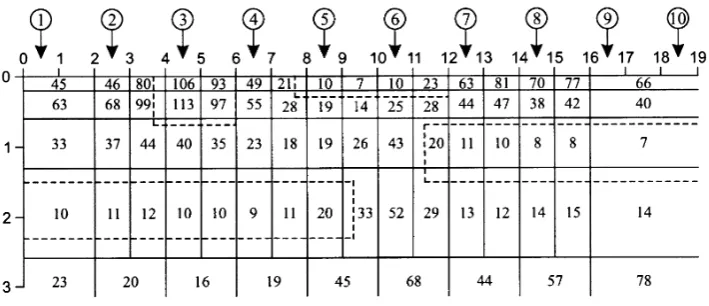
Fig. 1. Demonstration model for equality and inequality constraints (reproduced from Sasaki, 1989).
Fig. 2. Inversion result of synthetic MT data calculated for the model in Fig. 1. All blocks are constrained to positive values of resistivity in the inversion.
Let us define a new parameterxto introduce the a priori constraint, i.e.,
x =ln
m−a b−m
. (16)
Note that the subscripti is dropped in Eq. (16). Then the
perturbation ofx required in the inversion process is given by
δx= b−a
(m−a)(b−m)δm. (17)
Once the updating vectorδxis obtained, the initial parameter vectorx0will be updated as
x=x0+δx, (18)
and the parameters are renewed as
mupdated=a(b−m0)+b(m0−a)e
δx
(b−m0)+(m0−a)eδx
, (19)
wherem0indicates the initial parameter value.
4.
Numerical Examples
In order to verify the validity of the equality and inequal-ity constraints, we used Sasaki’s (1989) model as shown in
Fig. 1. The model consists of three low-resistivity bodies (5, 5, and 10·m) and a higher resistivity (100·m) body in a half-space of 50·m. Ten MT stations are sited with a spac-ing of 2 km and apparent resistivity data are generated for nine frequencies (0.1–50 Hz) at each site to yield a total of 90 data points. The model used for the smoothness-constrained inversion has 73 blocks as shown by the thin solid lines. The inversion scheme used in this study is basically the same as Sasaki (1989); The Lagrange multiplierλisfixed to 0.3 and no artificial noise is added in the inversion experiment. The primary difference lies in the form of roughness measure;
he used the gradient-amplifying factor αi to represent the
roughness term, while we did not use the factor (i.e.,αiwas
fixed to 1.0).
Figure 2 shows the inversion result obtained after three it-erations. The reconstructed resistivity section is nearly iden-tical to that of Sasaki (1989). The residual error was reduced from 0.61 to 0.11 and changed insignificantly after three it-erations. In the inversion all the resistivity parameters are constrained to positive values.
exam-Fig. 3. Inversion result with equality constraint excluding the shaded block from unknown parameters.
Fig. 4. Inversion result with equality constraint modifying the roughness terms of shaded blocks.
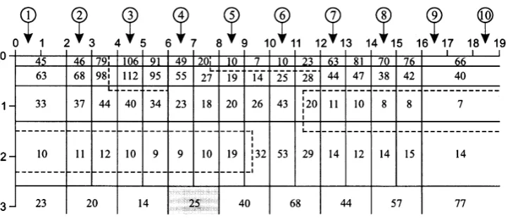
Fig. 5. Inversion result with inequality constraint. The resistivity of shaded block is bounded by 20 and 200·m in the inversion.
ple of this parameterization is shown in Fig. 3, in which one of the bottom blocks is excluded from the model. Because
the excluded block (shaded in thefigure) has no effect on
the roughness term, the image around this block becomes rougher than that in Fig. 2.
A more balanced image can be obtained by introducing
mean that the image of Fig. 4 is superior to that of Fig. 3. The inequality constraint is convenient to use as well as
flexible to introduce ground information in comparison with the other constraints including the soft equality constraint (10). In addition, it can easily include the reliability of ground information by controlling the interval between the upper and lower bounds. Figure 5 gives an example of using the inequality constraint. The resistivity of the bottom block
(shaded in the figure) is bounded by 20 and 200 ·m in
the inversion process. Since the lower limit is selected to be greater than the estimated block resistivity in Fig. 2, the resistivity of the shaded block in Fig. 5 is slightly better evaluated than that in Fig. 2.
5.
Concluding Remarks
In electrical and EM problems, the logarithm of resistiv-ity is usually used instead of resistivresistiv-ity itself in the inverse process to obtain a stable inversion. This parameterization has an effect of completely excluding negative resistivities from consideration as possible solutions. In this paper the positiveness constraint has been generalized to include more powerful and convenient constraint of parameters with lower and upper bounds, which are not restricted to positive values. The interval of two bounds reflects the reliability of ground information in this inequality constraint. In addition, the in-equality constraint approaches to the in-equality constraint if the width of two bounds becomes small. This generalized
constraint is helpful not only to stabilize the inversion pro-cess but also to include useful ground information through well logging and surface geology survey.
Acknowledgments. This research was partly supported by the U.S. Environmental Protection Agency and the Korea Science and En-gineering Foundation (No. 981-0403-009-2). Thoughtful reviews were provided by Yutaka Sasaki and Toshihiro Uchida.
References
Constable, S. C., R. L. Parker, and C. G. Constable, Occam’s inversion: A practical algorithm for generating smooth models from electromagnetic sounding data,Geophysics,52, 289–300, 1987.
deGroot-Hedlin, C. and S. Constable, Occam’s inversion to generate smooth, two-dimensional models from magnetotelluric data,Geophysics, 55, 1613–1624, 1990.
Rijo, L., W. H. Pelton, E. C. Feitosa, and S. H. Ward, Interpretation of apparent resistivity data from Apodi Valley, Rio Grande Do Norte, Brazil, Geophysics,42, 811–822, 1977.
Sasaki, Y., Two-dimensional joint inversion of magnetotelluric and dipole-dipole resistivity data,Geophysics,54, 254–262, 1989.
Tarantola, A.,Inverse Problem Theory: Methods for Data Fitting and Model Parameter Estimation, 613 pp., Elsevier, Amsterdam, 1987.
Tikhonov, A. N. and V. Y. Arsenin,Solutions of Ill-posed Problems, 258 pp., Winston & Sons, Washington, D.C., 1977.
Uchida, T., Smooth 2-D inversion for magnetotelluric data based on statis-tical criterion ABIC,J. Geomag. Geoelectr.,45, 841–858, 1993.