Development of a kinematic GNSS Acoustic positioning method based on a state space model

(1)

FULL PAPER

Development of a kinematic GNSS-Acoustic

positioning method based on a state-space

model

Fumiaki Tomita

1,2*

_{, Motoyuki Kido}

3

_{, Chie Honsho}

4

_{and Ryo Matsui}

4

Abstract

GNSS-A (combination of Global Navigation Satellite System and Acoustic ranging) observations have provided important geophysical results, typically based on static GNSS-Acoustic positioning methods. Recently, continuous GNSS-Acoustic observations using a moored buoy have been attempted. Precise kinematic GNSS-Acoustic position-ing is essential for these approaches. In this study, we developed a new kinematic GNSS-A positionposition-ing method usposition-ing the extended Kalman filter (EKF). As for the observation model, parameters expressing underwater sound speed struc-ture [nadir total delay (NTD) and underwater delay gradients] are defined in a similar manner to the satellite geodetic positioning. We then investigated the performance of the new method using both the synthetic and observational data. We also investigated the utility of a GNSS-Acoustic array geometry composed of multi-angled transponders for detection of vertical displacements. The synthetic tests successfully demonstrated that (1) the EKF-based GNSS-Acoustic positioning method can resolve the GNSS-GNSS-Acoustic array displacements, as well as NTDs and underwater delay gradients, more precisely than those estimated by the conventional kinematic positioning methods and (2) precise detection of vertical displacements can be achieved using multi-angled transponders and EKF-based GNSS-Acoustic positioning. Analyses of the observational data also demonstrated superior performance of the EKF-based GNSS-Acoustic positioning method, when assuming a laterally stratified sound speed structure. Further, we found three superior aspects to the EKF-based array positioning method when using observational data: (1) robustness of the solutions when some transponders fail to respond, (2) precise detection for an abrupt vertical displacement, and (3) applicability to real-time positioning when sampling interval of the acoustic ranging is shorter than 30 min. The precision of the detection of abrupt steps, such as those caused by coseismic slips, is ~ 5 cm (1σ) using this method, an improvement on the precision of ~ 10 cm of conventional methods. Using the observational data, the underwater delay gradients and the horizontal array displacements could not be accurately solved even using the new method. This suggests that short-wavelength spatial heterogeneity exists in the actual ocean sound speed structure, which cannot be approximated using a simple horizontally graded sound speed structure.

Keywords: GNSS-A positioning, Seafloor geodesy, Extended Kalman filter, Real-time positioning

(http://creat iveco mmons .org/licen ses/by/4.0/), which permits unrestricted use, distribution, and reproduction in any medium,

provided you give appropriate credit to the original author(s) and the source, provide a link to the Creative Commons license, and indicate if changes were made.

Introduction

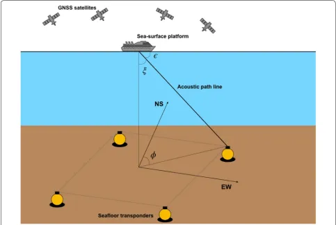
The GNSS-Acoustic (GNSS-A) positioning method, which was contrived by the Scripps Institute of Ocean-ography (Spiess 1985; Spiess et al. 1998), is a combi-nation technique of kinematic GNSS positioning on a

sea surface platform and underwater acoustic ranging between the sea-surface platform and a seafloor acous-tic benchmark (Fig. 1). The GNSS-A observations enable measurement of seafloor displacements in a global geo-detic coordinate system. The system has provided impor-tant geodetic observation results including detection of interseismic (e.g., Gagnon et al. 2005; Tadokoro et al. 2012; Yokota et al. 2016), coseismic (e.g., Tadokoro et al.

Open Access

*Correspondence: [email protected]

2_{Present Address: Japan Agency for Marine-Earth Science} and Technology, Yokohama, Japan

(2)

2006; Sato et al. 2011; Kido et al. 2011), and postseismic (e.g., Watanabe et al. 2014; Tomita et al. 2015, 2017; Hon-sho et al. 2019) deformation associated with earthquake cycles in subduction zones, and plate motions near ridge-transform boundaries (Chadwell and Spiess 2008).

Although GNSS-A observations are typically collected by campaign-style surveys using a research vessel as the sea surface platform, continuous GNSS-A observations have recently been developed using moored buoys (e.g., Imano et al. 2015; Kido et al. 2018; Kato et al. 2018; Imano et al. 2019) for an early warning system through instant offshore geodetic positioning. To support these efforts, we investigate a precise “kinematic” GNSS-A position-ing method. Most recently developed GNSS-A posi-tioning methods were designed as a “static” posiposi-tioning method, estimating a single positioning solution using long-term (over several hours) campaign survey data (e.g., Fujita et al. 2006; Ikuta et al. 2008; Honsho and Kido 2017; Yokota et al. 2018). Although the classic GNSS-A positioning method (Spiess et al. 1998; Kido et al. 2006) can be used to estimate a kinematic solution from a sin-gle acoustic ping, each solution has tens of centimeters of

positioning error due to spatio-temporal fluctuations in the underwater sound speed structure (SSS). However, it should be noted that it is possible to obtain a comparable solution with static GNSS-A positioning by averaging the kinematic solutions from long-term observational data (e.g., Kido et al. 2006; Tomita et al. 2015). Furthermore, the kinematic positioning method is useful for the detec-tion of temporally noisy data and for determining a final solution without using the noisy data. Thus, the classic positioning method is still an effective technique and has provided important observational results (e.g., Gagnon et al. 2005; Tomita et al. 2017).

As noted above, a major source of GNSS-A positioning error is thought to be the spatio-temporal fluctuations in underwater SSS. In past studies, a laterally stratified SSS has been assumed, and this assumption is generally applicable (e.g., Kido et al. 2008). If horizontal hetero-geneity in SSS is present, systematic positioning errors will arise. Additional file 1: Figure S1 shows a schematic image that a horizontally graded SSS (simple case of the horizontal heterogeneity in SSS) produces systematic bias in positioning results. As a response to this, static

(3)

GNSS-A positioning methods that consider the horizon-tally graded structure of underwater sound speeds that are persistent over the long-term (over several hours) have recently been developed (e.g., Yasuda et al. 2017; Yokota et al. 2018; Honsho et al. 2019), and have dem-onstrated some reduction in biased positioning errors. However, it has been found that short-term fluctuations in the horizontal heterogeneity of the SSS can be caused by internal gravitational waves (e.g., Spiess et al. 1998; Kido et al. 2006; Tomita et al. 2015), and these short-term fluctuations have degraded the precision of the kinematic GNSS-A positioning method.

In this study, we attempt to develop a kinematic GNSS-A positioning method based on a state-space model using the extended Kalman filter (EKF) (Kalman 1960) to improve the precision of the kinematic GNSS-A posi-tioning method. The Kalman filter (KF) has frequently been used in GNSS positioning systems to precisely estimate GNSS antenna position, tropospheric delay, ionospheric delay and other parameters (e.g., Lichten and Border 1987). Since the KF can constrain the behav-ior of time-dependent unknown parameters based on a given stochastic processes, it is a useful tool for kinematic inversion techniques. In this study, we first formulate the spatio-temporal fluctuations in the SSS for the GNSS-A positioning, based on the formulation for the tropo-spheric delay in the satellite geodetic measurements. Subsequently, we apply the above formulation to the EKF framework. Then we investigate the performance of this EKF-based approach using synthetic tests, and finally we apply the approach to observational data from the off-Tohoku region (northeast Japan).

Method

Principles of the GNSS‑A positioning method

A conceptual model of the GNSS-A observation sys-tem is shown in Fig. 1. The seafloor benchmark for each GNSS-A observation site is composed of several (~ 3–6) transponders forming a triangular- or square-shaped array. In the surveys, first, the position of a GNSS antenna attached to the sea-surface platform was measured using a kinematic GNSS positioning tech-nique. We then determined the position of an acous-tic transducer attached to the sea-surface platform from the GNSS antenna positions, the relative position between the GNSS antenna and the acoustic trans-ducer, and the attitude of the sea-surface platform. As well as positioning the acoustic transducer, the acoustic transducer transmits an acoustic signal and receives the returned acoustic signal from the seafloor transpond-ers; thus, round-trip travel times between the sea-sur-face acoustic transducer and the seafloor transponders

were obtained. We finally estimated the positions of the seafloor transponders by an iterative non-linear least means square technique minimizing residuals between the observed travel times and the calculated travel times (e.g., Spiess et al. 1998; Kido et al. 2006; Fujita et al. 2006; Ikuta et al. 2008).

One of the most important assumptions of the GNSS-A analysis is the rigid movement of the seafloor transponder array. Since an individual seafloor tran-sponder position can be estimated using the acoustic travel-time data collected by a “moving survey” (the acoustic pings are transmitted from various sea-surface points) (e.g., Ikuta et al. 2008; Honsho and Kido 2017; Additional file 1: Figure S2a), as similar to the deter-mination of the seismological hypocenter (e.g., Hirata and Matsu’ura 1987), we can determine array geometry composed of the transponders. Then, constraining the array geometry, array displacements relative to the pre-determined array position can be precisely estimated (e.g., Spiess et al. 1998; Kido et al. 2006; Matsumoto et al. 2008; Honsho and Kido 2017; Chen et al. 2018; Tadokoro et al. 2018b). If the array geometry is well determined, an array displacement can be estimated using only a single acoustic ping which simultaneously transmits to all seafloor transponders (e.g., Spiess et al. 1998; Kido et al. 2006; Additional file 1: Figure S2b). This type of the GNSS-A positioning, using individual pings, previously introduced as the classic GNSS-A positioning method in “Introduction” and often called “array positioning”, can in principle be achieved using the kinematic GNSS-A positioning method. Note that observational data collected from “point surveys” (where the acoustic pings are transmitted from the center of the seafloor transponder array) are required for kinematic GNSS-A positioning because accuracy of the array displacements degrades away from the array center (e.g., Kido 2007; Imano et al. 2015, 2019). In the following sections, we introduce a kinematic GNSS-A positioning method based on array positioning where the array geometry is already determined.

The observation equation analogy to satellite measurements

(4)

method assuming a horizontally graded SSS, we formu-lated the underwater delay gradient of sound speed based on the azimuthal dependence, as similar to the expres-sion of the tropospheric delay gradient in the satellite geodetic measurements (e.g., MacMillan 1995).

For the assumption of a laterally stratified SSS, the observation equation expressing a round-trip travel time for the seafloor transponder k at time tn is written as

follows:

with

where T_kobs_,_n and T_kcal_,_n represent an observed and calculated travel time, respectively. The travel time is calculated from the initial transponder position, pk , and the array

displacement, δpn . dn represents the position of a sea-surface acoustic transducer at time tn and v0 represents the initial sound speed profile. NTDn represents the NTD for time tn and Mǫk,n

represents the mapping function for NTD, which depends on an inclination angle ǫk,n of the acoustic ray path (Fig. 1). In this study, we adopted a simple mapping function using the sin function (Marini 1972):

This mapping function can also be represented using a shot angle of the acoustic ray path, ξk,n , which is the same

formulation of the array positioning introduced by Kido et al. (2006, 2008). In Eq. (1), the unknown parameters for each time step are the three-dimensional array displace-ment, δpn , and NTD. This observation equation is similar

to that presented in Kido et al. (2006, 2008), but we newly introduced a vertical component for the array displace-ment, δpZn , as an unknown parameter. The vertical array

displacement cannot be determined from kinematic array positioning using the point survey data at conven-tional GNSS-A sites because of the trade-off between vertical array displacements and the changes in sound speed (NTDs) (Additional file 1: Figure S3a). Thus, the conventional kinematic array positioning method fixes the vertical motion and estimates only the horizontal motions. Meanwhile, it is known that the moving survey data are essential to detect displacements in the vertical component (e.g., Sato et al. 2013) because the variation in shot angle of the seafloor transponders obtained from the

(1)

T_kobs_,_n =T_kcal_,_n(pk+δpn;dn;v0)+Mǫk,n

NTDn

(2)

pk =

pEW_k ,pNS_k ,pZ_kT,

(3) δpn=

δpEW_n ,δpNS_n ,δpZ_nT,

(4)

M

ǫk,n

= 1

sinǫk,n

= 1

cosξk,n

.

moving survey is required to solve the trade-off relation-ship. At some recent GNSS-A observation sites, six tran-sponders have been used to form a combination of small and large triangular arrays (Kido et al. 2015), providing variation in the shot angles even for a point survey (Addi-tional file 1: Figure S3b). Thus, we can detect the verti-cal array displacement even when using kinematic array positioning for a site with “multi-angled transponders”. The effects of using the multi-angled transponders are investigated in “Synthetic test” and “Application”.

For the assumption of a horizontally graded sound speed structure, the observation equation expressing a round-trip travel time for the seafloor transponder, k , at time, tn , is written as follows:

where GEW

n and GNSn represent the underwater delay gra-dients for the east–west and north–south components, respectively. φk,n is the azimuth of the seafloor

tran-sponder from the sea-surface platform at time, tn . This formulation for the underwater delay gradient is the same as that for the tropospheric delay gradient in the satel-lite geodetic measurements (MacMillan 1995). Although Kido (2007) proposed a formulation for describing the contributions to the sound speed gradient similar to our own formulation, the formulation of Kido (2007) did not account for the effect related to each seafloor transponder depth, represented by cotǫ_k,n in Eq. (5). Thus, our formu-lation is an updated version of Kido (2007). Yasuda et al. (2017) and Yokota et al. (2018) present alternative for-mulations for the sound speed gradient. However, their formulations necessitate that the acoustic ranging data must be collected from various sea-surface shot points by moving the sea-surface platform; therefore, they are unsuitable for use in kinematic positioning. Our formu-lation is suitable for use in kinematic positioning, but it should be noted that the sea-surface platform should be kept in position above the array center to obtain good resolution as pointed out by Kido (2007).

Application to the extended Kalman filter

We apply the above observation equation for the kin-ematic GNSS-A positioning to EKF. Since an inversion problem in the GNSS-A positioning is non-linear, EKF is utilized in this study. This non-linear state space model is governed by a system model (state transition equation) defined as

(5)

T_kobs_,_n =T_kcal_,_n(pk+δpn;dn;v0)+M

ǫk,n

NTDn

+M

ǫk,n

cotǫk,n

G_nEWsinφk,n+GNSn cosφk,n

,

(6)

(5)

and the observation model (observation equation) is defined as

where yn and xn are the observation vector and the state vector at time, tn , respectively. un is the control input

vector, vn is the process noise vector and wn is the meas-urement error vector. Since the EKF assumes that the processing noise and measurement errors follow the Gaussian distribution, their probability density functions are denoted as follows:

and

The process noise vector, vn , is under the Gaussian

noise with average zero and the covariance matrix (the process noise matrix), Qn . The measurement error, wn ,

is under the Gaussian noise with average zero and the covariance matrix, Rn . Fn and Hn in Eqs. (6) and (7) are the non-linear functions for calculating the state transi-tion and the synthetic observatransi-tions from the state param-eters, respectively. When a linear state space model is assumed for the system model, Eq. (6) is reformulated using a linear transition matrix, _F¯

n , as follows:

In the EKF, Hn is linearized based on a first-order

Tay-lor expansion in the neighborhood of the state x¯n pre-dicted from the system model:

with the linearized Jacobian matrix

Using the linearized matrix, the EKF can be applied in the same way as the linear KF; an update of the state parameters from the actual observation data based on the observation equation and a prediction of the state parameters based on the system model are performed alternately and iteratively at each time step. The pre-dicted state parameter xn+1 is obtained using the esti-mated state parameter of the previous time step xˆn by the

system model as shown in the following equation:

The predicted covariance matrix, _P¯_n+_{1 , is obtained}

using the estimated covariance matrix at the previous time step, _Pnˆ _{, using the following equation:}

(7)

yn=Hn(xn)+wn,

(8)

p(vn)∼N(0, Qn)

(9)

p(wn)∼N(0, Rn).

(10)

xn+1= ¯Fnxn+un+vn.

(11)

Hn(xn)=Hn(x¯n)+ ¯Hn(xn− ¯xn)

(12)

¯

Hn= ∂Hn(xn)¯ ∂xn¯ .

(13)

¯

xn+1= ˜Fnxˆn+un.

(14)

¯

Pn+1=FnPˆnFnT+Qn.

The estimated state parameter xnˆ is obtained using

the predicted state parameter x¯n using the following

equation:

where Kn is the Kalman gain, with

The updated covariance matrix is then obtained using the following equation:

For the assumption of a laterally stratified sound speed structure, the state vector is defined as

We assume the white noise in the stochastic pro-cess for the estimation of the array displacement, while we assume the random walk in the stochastic process for estimating NTD. The assumption of the white noise process for estimation of the array displacement is introduced to estimate these parameters in a kinematic manner, independent of time. The assumption of a ran-dom walk process for estimation of the NTD is often used for modeling the tropospheric delay in satellite measurements (e.g., Herring et al. 1990). The assump-tions are implemented by defining the linear transition matrix, F , as

and by defining the process noise matrix as

with

The variance used in the process noise matrix should be assigned in advance. As explained later in this section, the variance for the NTD, σ_NTD2 , is determined by fitting to the

observational data. The variance of the array displacements is assumed to be 1.0 m2_{since the array displacements can}

be estimated even for large abrupt displacements by assign-ing large values to the variance in the array displacements. Note that, to adjust the average levels of the array displace-ments using initial array displacedisplace-ments, δp0 , we define the control input vector as follows:

(15)

ˆ

xn= ¯xn+Knyn−Hn(x¯n),

(16)

Kn= ¯PnH¯T_nHn¯ Pn¯ H¯T_n +Rn−1.

(17)

ˆ

Pn=I+KnHn˜ Pn.¯

(18) xn=(δpn,NTDn)T=

δpEW_n ,δp_nNS,δpZ_n,NTDn

T

.

(19)

F=diag(0, 0, 0, 1)

(20)

Qn=diagσ_p2EW,σ_p2NS,σ_p2Z,�tnσ_NTD2

(21)

tn=tn−tn−1.

(22)

un≡u=(δp0, 0)T=

(6)

Unifying Eqs. (18)–(22), the system model [Eqs. (8) and (10)] for the assumption of a laterally stratified sound speed structure is defined. As for the observation model, the observation vector is obtained as

where kn is the total number of the replied seafloor

tran-sponders at time, tn . The non-linear Jacobian matrix is

defined as

and the linearized Jacobian matrix is defined via Eq. (12) as

We assume the same weight among the observed round-trip travel times regardless of the time step as follows:

where σ2 corresponds to variance of the measurement

errors for the round-trip travel times. Considering that the precision of the acoustic ranging is < ~1 cm (e.g., Fuji-moto 2014) and that the precision of the kinematic GNSS positioning on the sea-surface platform is roughly a few centimeters (e.g., Sugimoto et al. 2009), σ2 is assumed to

be 1.0 × 10−9 s2, which corresponds to an ~ 5 cm

meas-urement error in the line-of-sight direction.

For the assumption of a horizontally graded sound speed structure, we define the state vectors as

(23)

Similar to the assumptions for a laterally stratified sound speed structure, the array displacements are assumed to be a white noise process, while the NTD is assumed to be a random walk process. Further, the underwater delay gradient is assumed to be a random walk processes, like the tropospheric delay gradients in the satellite measurements (e.g., Bar-Server et al. 1998). Then, as for the system model, the transition matrix and the process noise matrix are defined as follows:

The variance in the array displacements and the NTD is the same as for the case of the laterally stratified sound speed structure. The variance in the underwater delay gradients are determined to fit the observational data, as for that of the NTD. To adjust the average levels of the array displacements using the initial array displacements, δp0 , we also define the control input vector as

As for the observation model, the observation vector is obtained using Eq. (23). The kth component of the non-linear Jacobian matrix Hn(xn) is defined as

and the linearized Jacobian matrix is defined as

We also assume the same covariance matrix for the measurement errors using Eq. (26).

The optimal variance for the process noise of the NTD is determined by maximizing likelihood. Given the variance parameter vector as

(7)

for the case of the horizontally graded SSS (for the case of the laterally stratified SSS, the variance parameter is

σ_NTD2 , not forming a vector), the log-likelihood is

writ-ten as follows (e.g., Kitagawa 2005; Segall and Matthews 1997):

with

Synthetic test Model setting

To evaluate the performance of the introduced EKF-based array positioning method, we conducted synthetic tests. We analyzed synthetic observational data assum-ing a horizontally graded SSS with a temporal fluctuation by both the conventional array positioning (e.g., Kido et al. 2006; Kido 2007) method and the EKF-based array positioning method. Note that we performed the above analysis assuming both a laterally stratified SSS and the horizontally graded SSS to investigate how the tempo-rally fluctuating gradient structure affects estimations compared with the case of a laterally stratified SSS. Syn-thetic round-trip travel-time data were produced based on the observation equation [Eq. (5)] by temporally vary-ing the unknown parameters

δpn,NTDn,GEW_n ,G_nNS as follows:

To calculate the synthetic travel-time data, we speci-fied the initial positions of the transponders, pk , synthetic

positions of an acoustic transducer at a sea-surface plat-form, dn , and an initial sound speed profile, v0 , as syn-thetic observational data.

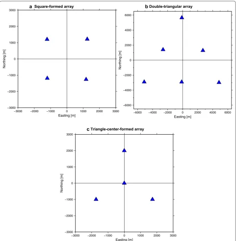
We generated synthetic observational data based on three different geometries for the seafloor transponder array (i.e., the initial positions of the transponders, pk ):

four transponders forming a square array geometry (Fig. 2a); six transponders forming a combined large and small triangular array (Fig. 2b); four transponders form-ing a combined triangular array with an additional tran-sponder at its center (Fig. 2c). The square-formed array geometry is the most popular pattern among the recently established GNSS-A sites in Japan, and the double-trian-gular array geometry has been adopted at five sites on a trial basis, which provides a multi-angled transponder array (e.g., Kido et al. 2015). The assumed geometries

(34)

L |y

= −1

2

Nlog 2π+

N

n=1

log|Vn| + N

n=1

yn−Hn(xn)TVn−1

yn−Hn(xn)

(35)

Vn= ¯HnPnH¯Tn +Rn.

(36)

T_ksys_,_n =T_kcal_,_n(pk+δpn;dn;v0)+M

ǫk,n

NTDn

+M ǫk,n

cotǫk,n

GEW_n sinφk,n+GnNScosφk,n

.

for the square-formed array (Fig. 2a) and for the double-triangular array (Fig. 2b) are same with actual observa-tion sites, the G08 (water depth: 3473 m) and G19 (water depth: 5725 m), located in the off-Tohoku region (Tomita et al. 2017), respectively. The triangular-centered array

geometry (Fig. 2c) has not yet been trialed. However, it can be treated as a multi-angled transponder site using only four transponders as illustrated in Fig. 2c; we inves-tigate its performance. Note that we assumed 4000 m of water depth for the synthetic triangular-centered array geometry.

Synthetic positions for an acoustic transducer on a sea-surface platform, dn , were generated within a radius of 50 m from the array center, imitating a point survey. Note that the actual positions of the sea-surface acoustic trans-ducers were used to calculate the synthetic travel-time data; however, when estimating the unknown parameters in the synthetic tests, we used positions for the sea-sur-face acoustic transducers contaminated by GNSS posi-tioning errors, with standard deviation of 3 cm for each component. These values where chosen as the precision of the kinematic GNSS positioning on the sea-surface platform is roughly a few centimeters (e.g., Sugimoto et al. 2009).

The initial sound speed profile, v0 , for each site (G08 and G19) was calculated from temperature and salin-ity data obtained from the World Ocean Atlas 2013 (WOA13; Locarnini et al. 2013; Zweng et al. 2013). WOA13 distributed average underwater structure mod-els for temperature, salinity and other indexes, complied with observational data over the past 60 years. We cal-culated a temperature and salinity profile for each site and converted them into a sound speed profile following Chen and Millero (1977). The initial sound speed profile for the triangular-centered array geometry is same as that for G17 site also located in the off-Tohoku region, at water depth of 4232 m.

(8)

a sine wave with an amplitude of 0.1 ms and a period of 2 h. The north–south component of the underwater delay gradient, GNSn , was fixed in time.

Based on the above model setup, we calculated the syn-thetic travel-time data using Eq. (36). In this calculation, a total of 300 shots of the synthetic acoustic pings were sampled at intervals of 60 s. Finally, we added measure-ment errors to the travel-time data assuming Gaussian

noise with a standard deviation of 1.0 × 10−5 s

(corre-sponding to ~ 0.75 cm in the one-way slant path) since precision of the acoustic ranging is < ~ 1 cm (e.g., Fuji-moto 2014).

Results

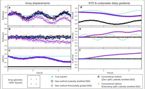
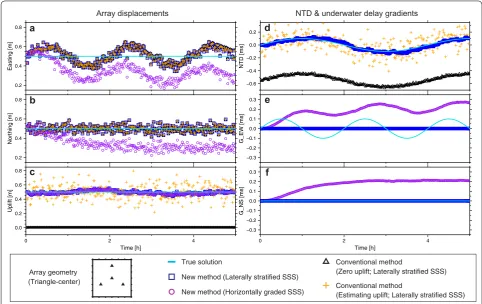
Figure 3 shows the kinematic array positioning results for the synthetic data assuming the square-formed array a Square-formed array b Double-triangular array

c Triangle-center-formed array −3000

−2000 −1000 0 1000 2000 3000

Northing [m

]

−3000 −2000 −1000 0 1000 2000 3000 Easting [m]

−6000 −4000 −2000 0 2000 4000 6000

Northing [m

]

−6000 −4000 −2000 0 2000 4000 6000 Easting [m]

−3000 −2000 −1000 0 1000 2000 3000

Northing [m

]

−3000 −2000 −1000 0 1000 2000 3000 Easting [m]

(9)

geometry. The solutions estimated by the conventional array positioning method, which fixed the vertical array displacements to be zero (e.g., Kido et al. 2006, 2008) (black triangles), demonstrated a time-dependent sys-tematic error in the east–west component of the array displacements (Fig. 3a), caused by the prescribed gra-dient in SSS (Fig. 3e). Since the vertical array displace-ments are fixed to be zero (Fig. 3c), the estimated NTDs are biased from the true solutions; however, the esti-mated NTDs could explain the true temporal evolution (Fig. 3d). The solutions obtained by the conventional array positioning method, estimating both vertical and horizontal array displacements, are shown by orange crosses. The estimated vertical array displacements are out of plotting range in Fig. 3c, with displacements of up to ± ~ 10 m. As the estimated NTDs are also out of plot-ting range in Fig. 3d, the trade-off relationship between the vertical array displacements and the NTDs cannot be solved in the square-formed array geometry when only conducting a point survey. Further, the unsolved NTDs

might degrade the precision of the horizontal array dis-placements (Fig. 3a, b). The EKF-based array position-ing, assuming a laterally stratified SSS (blue squares), prevents the vertical array displacements and the NTDs from diverging. However, the trade-off cannot be solved even when using the EKF-based array positioning, mean-ing that the vertical array displacements and the NTDs deviated from the true values over time. The horizontal components of the array displacements are almost the same as the solutions obtained from the conventional array positioning method with fixed vertical array dis-placements (Fig. 3a, b) since the NTDs did not diverge through the EKF-based array positioning in this time window. Estimation results of the EKF-based array positioning assuming a horizontally graded SSS (pur-ple circles) showed similar vertical array displacements and NTDs to predictions assuming a laterally stratified SSS (Fig. 3c, d). In the EKF-based array positioning, the horizontal components of the array displacements also deviated from the true values with time because of the

a

New method (Laterally stratified SSS)

New method (Horizontally graded SSS)

Conventional method

(Zero uplift; Laterally stratified SSS)

Conventional method

(Estimating uplift; Laterally stratified SSS)

(10)

trade-off relationship between the array displacements and the underwater delay gradients (Fig. 3a, b).

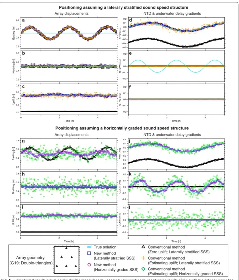
Figure 4 shows the kinematic array positioning results for the synthetic data assuming the double-triangle array geometry. The conventional array positioning method of fixed zero vertical array displacements showed similar results to the case of the square-formed array geometry (black triangles in Fig. 4a–l), but for this new geometry, the conventional array positioning method was also able to resolve the vertical array displacements and the NTDs (orange crosses in Fig. 4a–f). This improvement is a result of the multi-angled transponders solving the ver-tical array displacements with the NTDs as explained in “The observation equation analogy to satellite

measure-ments”. Furthermore, the EKF-based array positioning

method, assuming the laterally stratified SSS, further demonstrates the superior performance for the vertical array displacements (blue squares in Fig. 4c) since the EKF provides a temporal constraint on NTDs that avoids numerical instability when solving the vertical array dis-placements and NTDs. The conventional array position-ing method [an updated method from Kido (2007) based on Eq. (5)] and the EKF-based array positioning method for the horizontally graded SSS are shown in Fig. 4g–l as green diamonds and purple circles, respectively. The conventional method approximately solves the gradient parameters (Fig. 4k, l), but the solutions of the gradient parameters and of the horizontal array displacements have large dispersions, probably because of the poten-tial trade-off relationship among them. Meanwhile, the EKF-based array positioning method stably solves those parameters by constraining the temporal evolution of the gradient parameters and greatly reduces the dispersion in the horizontal array displacements.

Figure 5 shows the kinematic array positioning results for the synthetic data assuming the triangu-lar-centered array geometry. The conventional array positioning method can resolve the vertical array dis-placements and the NTDs unlike for the case of the square-formed array geometry (orange crosses in Fig. 5c, d). However, note that the dispersion of the ver-tical array displacements is a little larger that the case of the double-triangular-formed array geometry prob-ably because of insufficient variation in the shot angles. The EKF-based array positioning method can improve the precision of the vertical array displacements (blue squares in Fig. 5c) by temporally constraining NTDs similar to the double-triangular-formed array geom-etry. Although the underwater delay gradients cannot be solved in the case of the triangular-centered array geometry (Fig. 5e, f), this geometry enables us to detect kinematic vertical array displacements accurately, using only four transponders (the double-triangular-formed

array geometry requires six transponders). Further-more, the precision of the vertical array displacements can be improved using the EKF-based array positioning method, assuming a laterally stratified SSS.

Through the synthetic test, we confirmed (1) the util-ity of the multi-angled transponders for detecting the kinematic vertical array displacements, (2) the accu-rate performance of the EKF-based array positioning method for precisely detecting the vertical array dis-placements at the multi-angled transponder sites, and (3) the accurate kinematic solutions to the underwater delay gradients for the double-triangular-formed array geometry site via the EKF-based array positioning method.

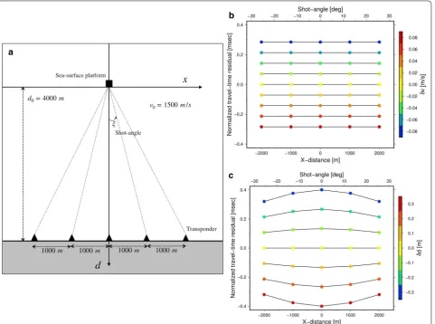
Point (1) shows the importance of acoustic data with various shot angles during a point survey. Effects of a temporal sound speed fluctuation can be expressed by NTDs that are independent of shot angles, whereas the vertical array displacement is sensitive to variation of shot angles. We validated this fact through a simple numerical test. We assumed a two-dimensional field as shown by Fig. 6a, and five transponders are vertically located. When perturbation is given in the average sound speed, the one-way travel-time residual can be expressed as follows:

Using the mapping function, contribution of the sound speed perturbation to the travel-time residual is common with each transponder. In other words, the travel-time residual normalized by the mapping function is inde-pendent of the horizontal distance of the transducer (i.e., shot angle) as follows:

Figure 6b shows the normalized travel-time residuals when various values of the sound speed perturbation are given. Figure 6b clearly demonstrates that the normal-ized travel-time residuals are same among the transduc-ers. Meanwhile, when perturbation in depth is given, the travel-time residual can be written as follows:

Then the normalized travel time can be also written as follows:

(37)

δT(δv)=T(v0+δv)−T(v0)=

x2₊_d2 0

₁

v0+δv−

1

v0

.

(38)

δTnormlized(δv)=δT(δv)/M(ǫ)=d0

1 v0+δv

− 1 v0

.

(39)

δT_(δd₎=T₍d₀+δd₎−T₍d₀₎

= 1

v₀

x2₊₍_d

0+δd)2−

x2₊_d2 0

(11)

0.2 0.4 0.6 0.8

Easting

[m

]

0.2 0.4 0.6 0.8

Northing

[m]

0.0 0.2 0.4 0.6 0.8

Uplif

t [m

]

4 2

0

Time [h]

0.2 0.4 0.6 0.8

Easting [m

]

0.2 0.4 0.6 0.8

Northing [m

]

0.0 0.2 0.4 0.6

0.8

Uplift [m

]

4 2

0

Time [h]

a

b

c

d

e

f

Positioning assuming a laterally stratified sound speed structure

Positioning assuming a horizontally graded sound speed structure

g

h

i

j

k

l

−0.5 −0.4 −0.3 −0.2 −0.1 0.0 0.1 0.2

NTD [ms]

−0.2 −0.1 0.0 0.1 0.2

G_EW [ms]

−0.2 −0.1 0.0 0.1 0.2

G_NS [ms]

4 2

0

Time [h]

−0.5 −0.4 −0.3 −0.2 −0.1 0.0 0.1 0.2

NTD [ms]

−0.2 −0.1 0.0 0.1 0.2

G_EW [ms]

−0.2 −0.1 0.0 0.1 0.2

G_NS [ms]

4 2

0

Time [h]

Array displacements NTD & underwater delay gradients

Array geometry (G19: Double-triangles)

True solution New method

(Laterally stratified SSS) New method

(Horizontally graded SSS)

Conventional method

(Zero uplift; Laterally stratified SSS) Conventional method

(Estimating uplift; Laterally stratified SSS) Conventional method

(12)

Figure 6c shows the normalized travel-time residu-als when various values of the perturbation in depth are given. Figure 6c demonstrates that the normalized travel-time residuals vary depending on the absolute horizontal distance from the array center (i.e., abso-lute shot angles). This indicates that if the absoabso-lute shot angles for the transponders from the array center are same (such as the square-formed array geometry), we cannot distinguish contributions of the sound speed perturbation from those of the depth perturbation. Thus, variation in absolute shot angles is essential to precisely estimate vertical displacements in the kin-ematic GNSS-A positioning.

In the next section, we apply the EKF-based array posi-tioning methods to actual observational data.

(40)

We used the actual GNSS-A observational data collected by Tomita et al. (2017) in the off-Tohoku region. We used the observational data collected on March 14, 2015, at the G08 site (longitude: 143.647°E, latitude: 38.721°N, depth: 3473 m) as an example of the square-formed array geometry (Fig. 7). Moreover, we used the observational data collected on February 28, 2015, at the G19 site (lon-gitude: 142.671°E, latitude: 36.496°N, depth: 5725 m) as an example of the double-triangular-formed array geom-etry (Fig. 8). The details of the observational data are shown in Tomita et al. (2017).

For GNSS positioning using the KF, the process noises are often assigned as fixed values (e.g., Bar-Server et al. 1998; Hirata and Ohta 2016) because there is high com-putational cost to determine the optimal process noise values. Therefore, it is worthwhile to search for “general” process noise values to use with the EKF-based GNSS-A array positioning method. From the synthetic tests, we have found that the double-triangular-formed array geometry is suitable for the EKF-based array position-ing method, regardless of the assumed SSS. Therefore,

(a)

Array geometry

Conventional method

(Estimating uplift; Laterally stratified SSS) a

(13)

we investigated the optimal process noise values by maxi-mizing the likelihood of the actual observational data, at sites with the double-triangular-formed array geometry. Thus, we also analyzed all the observational data at the sites forming the double-triangular-formed array geom-etry collected by Tomita et al. (2017): G04 (longitude: 143.897°E, latitude: 39.566°N, depth: 4587 m), G10 (longi-tude: 143.483°E, lati(longi-tude: 38.302°N, depth: 3271 m), G15 (longitude: 143.521°E, latitude: 37.677°N, depth: 5264 m) and G19 sites. Then we compared the determined pro-cess noise values.

Results

Figure 7 shows the kinematic array positioning results for the actual observational data at the G08 site (the square-formed array geometry). We analyzed the observational data using the conventional array positioning method of

fixed vertical array displacements (black triangles), the conventional array positioning method estimating the vertical array displacements as well as the horizontal array displacements (orange crosses), and the EKF-based array positioning method assuming a laterally strati-fied SSS (blue squares). The general features of the posi-tioning results are similar to the synthetic test results, assuming the square-formed array geometry (Fig. 3); the vertical array displacements could not be solved due to the trade-off relationship between the vertical array dis-placements and the NTDs, even by the EKF-based array positioning method, and the horizontal array displace-ments estimated by the EKF-based array positioning method were almost the same with those estimated by the conventional array positioning method of fixed verti-cal array displacements.

(14)

Figure 8a–f shows the kinematic array positioning results for the actual observational data at the G19 site (the double-triangular-formed array geometry) analyzed using the positioning method assuming a laterally strati-fied SSS. The general features of these positioning results are similar to those of the synthetic test for the double-triangular-formed array geometry (Fig. 4a–f); the hori-zontal components of the solutions estimated by this method are roughly in accordance. The vertical array displacements can be determined using the conventional array positioning method of estimated vertical array dis-placements (orange crosses) and the EKF-based array positioning method (blue squares). Moreover, the EKF-based array positioning method can detect the vertical array displacements more precisely than the conventional array positioning method. Although the horizontal array displacements estimated by the conventional array posi-tioning method of fixed vertical displacements agree well with those estimated using the EKF-based array position-ing method in the synthetic test (Fig. 4a, b), they some-times disagree for the actual observational data (black triangles in Fig. 8a, b). The causes of this are discussed later in “Robustness in the case of an unresponsive

transponder”. Unlike the synthetic test, the vertical array displacements estimated using the EKF-based array posi-tioning method fluctuate with time, and the fluctuation is up to a few tens of centimeters, although the vertical array displacements should be constant during the cruise; the causes of this are discussed later in “Improvements to detection of vertical array displacements”.

Features of the positioning results for the actual obser-vational data at the G19 site, analyzed using the posi-tioning methods assuming a horizontally graded SSS (Fig. 8g–l), are quite different from the results of the synthetic test (Fig. 4g–l). The horizontal components of the solutions showed large fluctuations with time in both cases of the conventional array positioning method (green diamonds) and of the EKF-based array positioning method (purple circles). The variations are larger than those observed from the solutions obtained assuming a laterally stratified SSS. These variations show short-term (~ a few hours) periodic fluctuations (non-random vari-ations); the degraded positioning results are attributed to systematic modeling errors in the underwater delay gradients. These modeling errors are discussed later in

“Sound speed structure in actual ocean”. Meanwhile,

−0.6

Array geometry

Conventional method

(15)

a

Positioning assuming a laterally stratified sound speed structure

Positioning assuming a horizontally graded sound speed structure

g

Array geometry

(Estimating uplift; Laterally stratified SSS) Conventional method

(16)

the estimated vertical array displacements and NTDs are almost the same as the solutions obtained assuming a laterally stratified SSS. Thus, the NTDs can be solved independently of the crucial modeling errors in the underwater delay gradients. Additional file 1: Figures S4– S8 show positioning results at the G19 site for the actual observational data collected from the other cruises, and the features of the positioning results mentioned above are also found in the results of other cruises.

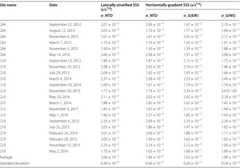
The process noise values determined from the actual observational data, for the double-triangular-formed array geometry, are summarized in Table 1. The opti-mal process noise values ( σ_NTD ) are determined to be

~ 2.0 × 10−3 (s/s1/2) regardless of the assumed SSS, the

observation site and the observation period. Thus, this value would be generally applicable. Although the pro-cess noise values of the underwater delay gradient were determined to be ~ 1.9 × 10−3 (s/s1/2) in both the east–

west and north–south components ( σ_GEW, σ_GNS ), these values are not reliable because the estimated horizontal

array displacements assuming a horizontally graded SSS were not accurately determined, as explained above.

Discussion

Performance of the EKF‑based array positioning method Here, we discuss the utility of our newly developed EKF-based array positioning method. As shown in “Results”, the EKF-based array positioning method, assuming a lat-erally stratified SSS, shows superior performance when compared to the conventional array positioning meth-ods. The advantages of the EKF-based array positioning method are (1) robust positioning accuracy even when some seafloor transponders are unresponsive; (2) pre-cise detection of the vertical array displacements; (3) applicability to continuous GNSS-A positioning. These advantages are discussed in this section. However, in instances of a horizontally graded SSS, the EKF-based array positioning method failed to improve on the preci-sion of the array positioning results, when compared to Table 1 Estimated process noise values using actual data at G04, G10, G15 and G19

The estimated process noise values are shown, and their units are all s/s1/2_{. The process noise values for NTD are shown in the both cases of the laterally stratified SSS}

(column 3) and the horizontally gradient SSS (column 4). The process noise values for underwater delay gradients in east–west and north–south components are shown in the case of horizontal gradient SSS (columns 5 and 6, respectively)

Site name Date Laterally stratified SSS

(s/s1/2₎ Horizontally gradient SSS (s/s 1/2₎

σ_NTD σ_NTD σ_G(EW) σ_G(NS)

G04 September 22, 2012 2.07 × 10−3 _2.06_×₁₀−3 _1.87_×₁₀−3 _2.10_×₁₀−3

G04 August 12, 2013 2.05 × 10−3 _1.79_×₁₀−3 _1.77_×₁₀−3 _1.69_×₁₀−3

G04 November 4, 2013 1.61 × 10−3 _1.61_×₁₀−3 _2.05_×₁₀−3 _2.17_×₁₀−3

G04 March 7, 2015 1.73 × 10−3 _1.74_×₁₀−3 _1.35_×₁₀−3 _1.41_×₁₀−3

G04 November 3, 2015 1.50 × 10−3 _1.50_×₁₀−3 _1.59_×₁₀−3 _1.88_×₁₀−3

G04 May 14, 2016 2.66 × 10−3 _2.58_×₁₀−3 _1.91_×₁₀−3 _2.08_×₁₀−3

G10 September 13, 2012 1.85 × 10−3 _1.87_×₁₀−3 _2.15_×₁₀−3 _1.72_×₁₀−3

G10 November 29, 2012 2.98 × 10−3 _2.42_×₁₀−3 _2.19_×₁₀−3 _1.86_×₁₀−3

G10 July 29, 2013 2.04 × 10−3 _1.62_×₁₀−3 _1.81_×₁₀−3 _1.66_×₁₀−3

G10 March 4, 2014 2.37 × 10−3 _2.28_×₁₀−3 _2.22_×₁₀−3 _2.48_×₁₀−3

G10 September 20, 2014 1.69 × 10−3 _1.67_×₁₀−3 _1.74_×₁₀−3 _1.74_×₁₀−3

G10 November 20, 2015 1.77 × 10−3 _1.74_×₁₀−3 _2.33_×₁₀−3 _2.41E₋₀₃

G10 May 20, 2016 2.11 × 10−3 _2.02_×₁₀−3 _2.42_×₁₀−3 _2.18_×₁₀−3

G15 March 1, 2014 1.88 × 10−3 _1.85_×₁₀−3 _1.67_×₁₀−3 _1.42_×₁₀−3

G15 November 9, 2015 1.81 × 10−3 _1.67_×₁₀−3 _2.11_×₁₀−3 _1.94_×₁₀−3

G15 May 7, 2016 1.85 × 10−3 _1.57_×₁₀−3 _1.85_×₁₀−3 _1.63_×₁₀−3

G19 September 6, 2012 2.33 × 10−3 _2.09_×₁₀−3 _2.19_×₁₀−3 _2.26_×₁₀−3

G19 July 25, 2013 2.05 × 10−3 _1.86_×₁₀−3 _1.97_×₁₀−3 _1.82_×₁₀−3

G19 February 26, 2014 3.01 × 10−3 _3.00_×₁₀−3 _1.80_×₁₀−3 _1.71_×₁₀−3

G19 February 28, 2015 2.05 × 10−3 _1.99_×₁₀−3 _1.62_×₁₀−3 _1.82_×₁₀−3

G19 November 15, 2015 2.19 × 10−3 _2.14_×₁₀−3 _2.15_×₁₀−3 _1.90_×₁₀−3

G19 May 2, 2016 1.70 × 10−3 _1.65_×₁₀−3 _1.68_×₁₀−3 _1.89_×₁₀−3

Average 2.06 × 10−3 _1.94_×₁₀−3 _1.93_×₁₀−3 _1.90_×₁₀−3

(17)

other methods. The causes of this failure are discussed in “Sound speed structure in actual ocean”.

Robustness in the case of an unresponsive transponder

The horizontal array displacements for the actual obser-vational data estimated using the conventional array positioning method with fixed vertical array displace-ments (black triangles in Fig. 8a, b) show little scatter when compared with those estimated using the conven-tional and the EKF-based array positioning methods. Fig-ure 9a, b also shows the horizontal array displacements for the same data estimated using the conventional array positioning method of fixed vertical array displacements, and the plotted color represents the number of the responding transponders for each ping. This illustrates that the scattered array displacements appear when some transponders are not responding. Such response fail-ures can arise for various reasons including, for example, significant background mechanical noise, bad weather and overlaps in the signal response. For examples, in the observational data obtained in March 2015 at G19 (Fig. 8), three transponders configuring the inner trian-gle well responded (data acquisition ratio is ~ 97 percent), while the other three transponders configuring the outer triangle occasionally failed to responded (data acquisi-tion ratio is ~ 83 percent). Yet in the observaacquisi-tional data obtained in November 2015 at G19 (Additional file 1:

Figure S7), all transponders well responded (data acquisi-tion ratio is ~ 97 percent).

To investigate the influence of the unresponsive tran-sponders, we performed additional synthetic test with intermittent transponder failures (Fig. 10). The condi-tions of these synthetic test are similar to those assum-ing the double-triangular-formed array geometry, but the temporal fluctuations in the underwater delay gradients are omitted (thus, the horizontal array displacements should be constant with time). In the test, 40% of the responses from the transponders are randomly excluded. Figure 10a–c shows the array displacements estimated using the kinematic array positioning method (true array displacements are 0.5 m for all components). As seen for the actual observational data (Fig. 8), the conventional (orange crosses) and the EKF-based (colored dots) meth-ods estimating the vertical array displacements generally detect true horizontal array displacements, whereas the conventional array positioning method of fixed vertical array displacements (black triangles) provides scattered solutions. However, assuming that the true vertical array displacements are zero, the conventional array posi-tioning method with fixed vertical array displacements successfully provides comparable horizontal array dis-placements (black triangles in Fig. 10d–e; note that they are totally overlapped with the colored dots). These syn-thetic tests suggest that deviation of the vertical array a

b

c

d

−0.2 0.0 0.2 0.4

E

asting

[m

]

−0.6 −0.4 −0.2 0.0 0.2 0.4

N

ort

hing

[m

]

0 2 4 6 8 10 12

Time [h]

1 2 3 4 5 6

Number of the responded transponder

s

Conventional method (Zero uplift; Laterally stratified SSS) New method(Laterally stratified SSS)

Array geometry (G19: Double-triangles)

−0.2 0.0 0.2 0.4

E

asting

[m

]

−0.6 −0.4 −0.2 0.0 0.2 0.4

N

ort

hing

[m

]

0 2 4 6 8 10 12

Time [h]

(18)

displacements from true values would produce crucial modeling errors in the horizontal array displacements when some transponders fail to respond. We considered that this modeling error is related to the apparent shift in the point of the array center when some transpond-ers fail to respond. Since the accuracy of the array posi-tioning degrades away from the array center (e.g., Kido 2007; Imano et al. 2015, 2019), deviation of the vertical array displacements results in serious modeling errors due to the apparent shift in the point of the array center. This problem can be avoided by estimating the vertical array positions precisely. Since the precision of the ver-tical array displacements estimated using the EKF-based array positioning method is better than that of the con-ventional array positioning method, the EKF-based array positioning method can stably perform the array posi-tioning not only for the vertical array displacements but also for the horizontal array displacements, as shown from the analyses of the actual observational data (e.g., Fig. 8a–c; Additional file 1: Figure S8a–c).

Figure 10 further illustrates the robustness of the EKF-based array positioning method in the instance of unre-sponsive transponders. In principle, the EKF-based array positioning method can estimate the unknown param-eters even when the number of observations is smaller than the number of unknown parameters. The colors of the dots (the solutions from the EKF-based array posi-tioning method) in Fig. 10 represent the number of unre-sponsive transponders; the EKF-based array positioning method can provide accurate solutions when more than three responsive transponders are available. When less than two responsive transponders are available, the array positions are estimated to be 0.3 m for all compo-nents, which corresponds to the initial array displace-ments for the control input in Eq. (30), as explained in “Model setting”. Therefore, the array displacements can-not be constrained using the observational data in this case. However, since the conventional array position-ing method requires more than four responsive tran-sponders to estimate the three components of the array

0.0

s

With an offset in vertical component Without an offset in vertical component

Array displcaments for synthetic incomplete data

Array geometry

s

*Color shows number of the responded transponders

Conventional method

(19)

position and NTDs (orange crosses in Fig. 10), the EKF-based array positioning method can increase positioning opportunities when only three responsive transponders are available.

Improvements in the detection of vertical array displacements

As shown both in the synthetic tests (Figs. 4, 5) and in the actual observational data analysis (Fig. 8; Additional file 1: Figures S4–S8), the EKF-based array positioning method successfully improves the precision of the array displacements, especially for the vertical component when using multi-angled transponders. However, unlike the synthetic tests, the positioning results using the actual observational data showed temporal fluctuations in the vertical array displacements of up to a few tens of centimeters (Fig. 8c; Additional file 1: Figures S4c–S8c). The primary reasons for this temporal fluctuation are (1) GNSS positioning errors on the sea-surface platform, and (2) deviation from a laterally stratified SSS in the actual ocean. Note that Earth tide effects were eliminated in the shown vertical positioning results in advance although the Earth tide potentially produces long-term fluctuation in the vertical component.

The GNSS positioning errors directly propagate to the positions of the acoustic transducers on the sea-surface platform and then propagate to the array displacements. Although it is difficult to evaluate positioning errors for this moving body, we can consider that the verti-cal positions of the acoustic transducer on the sea-sur-face platform are inherently bounded to the sea sursea-sur-face. Therefore, eliminating oceanic tidal effects and geoid heights from the acoustic transducer positions, we can roughly evaluate the relative temporal fluctuation of the vertical GNSS positioning errors, although the absolute GNSS positioning errors cannot be evaluated (Fujita and Yabuki 2003). The vertical positions of the acoustic transducers are shown as bold gray curves in Fig. 8c and Additional file 1: Figures S4c–S8c, eliminating the oce-anic tidal effects using the NAO.99Jb model (Matsumoto 2000) and the geoid heights calculated from Fukuda (1990). Note that the acoustic transducer positions are smoothed by a 5-min moving average filter because the positions are shaken by sea waves with short timescale. Since the long-term fluctuation in the vertical array posi-tions is consistent with that of the acoustic transducer positions, the GNSS positioning errors are considered to be the major source of error in the vertical array dis-placements. Table 2 shows 1σ standard deviations of the vertical array positions for the actual observational data estimated by the conventional array positioning method (columns 3–5) and by the EKF-based array positioning method (columns 6–8). The average standard deviation of

11.14 cm (column 6: std.) is reduced to 9.18 cm (column 7: corrected std.) by subtracting the acoustic transducer positions in the case of the EKF-based array position-ing method [the reduction can be up to ~ 5 cm in the observational data for G04 (March, 2015)]. Although one of the factors causing the long-term GNSS positioning errors is the very long baseline for kinematic differential GNSS positioning (e.g., Colombo et al. 2000), kinematic precise point positioning (PPP) (Zumberge et al. 1997) techniques, which do not require a terrestrial reference station, have improved and would be an alternative way of determining the position of the sea-surface platform. Watanabe et al. (2017) reported that kinematic PPP provided more stable solutions than long-baseline dif-ferential positioning. These developments in GNSS posi-tioning would enable us to further improve the precision of the vertical array displacements using the EKF-based array positioning to less than ~ 10 cm. It should be noted that the precisions discussed here are relative precisions in the half-day observation data, and are not the absolute accuracy of the vertical positions. To discuss the absolute accuracy, much longer observational data are required.

(20)

detect an abrupt step in the vertical component eliminat-ing the potential trade-off relationship between the verti-cal array displacements and the NTDs.

Applicability to real‑time GNSS‑A positioning

Our main finding, accurate detection of vertical displace-ments, comes from appropriate estimation of NTDs con-strained by the EKF. Although the constraint of temporal variations in NTDs can be achieved using conventional inversion techniques using a batch of acoustic ranging data (e.g., Honsho and Kido 2017), the EKF-based GNSS-A positioning method has an additional utility: instant processing suitable for real-time positioning.

The batch-type positioning requires high computa-tional cost because a significant amount of data should be simultaneously processed; however, the EKF-based GNSS-A positioning method can determine a posi-tion using only acoustic ranging data for each ping, when the process noise values are fixed, as shown in “Results”. In these circumstances, our method requires

less computational cost, comparable to the simplest kinematic GNSS-A positioning methods which do not provide temporal constraints of NTDs (e.g., Spiess et al. 1998; Kido et al. 2006). Furthermore, the EKF-based positioning method can provide kinematic solutions instantly, just after collection of the acoustic ranging data for each ping, because this technique does not need “future” acoustic ranging data to constrain the temporal variation in NTDs. Recently, some trials of real-time and continuous GNSS-A observations have been conducted using a moored buoy (e.g., Imano et al. 2015; Kido et al. 2018; Kato et al. 2018; Tadokoro et al. 2018a). In this application, kinematic GNSS-A positions are estimated using a small computer attached to the buoy, which are then transmitted to an onshore station via satellite relay. Thus, the computational cost of GNSS-A posi-tioning using a moored buoy is as low as possible. Our proposed method has a low computational cost and can provide a kinematic position with constraints on the temporal variation of NTDs, using real-time processing, Table 2 1σ standard deviations (std.) of the vertical array displacements assuming a laterally stratified SSS

Columns 3 and 6 (std.) show simple standard deviations for solutions in the vertical component, while columns 4 and 7 (corrected std.) show standard deviations for solutions in the vertical component corrected by subtraction of the acoustic transducer positions. Columns 5 and 8 (difference std.) show standard deviations for differential sequences of the solutions in the vertical component

Site name Date Conventional array positioning EKF‑based array positioning Std. (cm) Corrected std.

(cm) Difference std. (cm) Std. (cm) Corrected std. (cm) Difference std. (cm)

G04 September 22, 2012 10.23 7.32 4.41 10.05 7.02 3.15

G04 August 12, 2013 11.96 9.88 9.62 9.95 7.28 2.96

G04 November 4, 2013 12.50 10.72 4.17 12.10 10.24 2.44

G04 March 7, 2015 6.82 6.25 6.31 5.73 5.09 2.96

G04 November 3, 2015 7.13 7.98 5.34 6.48 7.48 3.85

G04 May 14, 2016 10.60 9.96 10.50 9.71 8.79 7.36

G10 September 13, 2012 17.83 14.30 12.81 14.18 8.29 3.93

G10 November 29, 2012 16.78 15.64 13.75 15.31 15.92 6.39

G10 July 29, 2013 14.95 12.13 8.27 13.54 10.87 3.94

G10 March 4, 2014 11.52 12.48 10.19 9.52 10.88 4.65

G10 September 20, 2014 8.43 7.08 5.40 8.09 6.45 3.14

G10 November 20, 2015 11.07 10.31 8.89 9.81 8.90 4.16

G10 May 20, 2016 13.65 12.35 9.98 12.50 11.25 5.73

G15 March 1, 2014 17.47 9.28 7.87 17.04 8.12 3.20

G15 November 9, 2015 10.99 11.70 11.02 8.12 8.97 3.97

G15 May 7, 2016 15.69 11.44 12.15 13.97 9.31 7.82

G19 September 6, 2012 13.47 12.40 10.58 14.59 16.00 5.85

G19 July 25, 2013 22.19 12.52 11.96 19.99 10.45 6.01

G19 February 26, 2014 11.23 8.46 5.87 10.83 7.94 3.59

G19 February 28, 2015 10.74 10.56 11.86 7.78 7.42 4.71

G19 November 15, 2015 9.22 8.07 8.27 7.97 6.50 4.24

G19 May 2, 2016 11.22 12.25 11.72 7.92 8.93 4.81

Average 12.53 10.59 9.13 11.14 9.18 4.50

(21)

making it suitable for real-time and continuous GNSS-A observations.

To estimate vertical positions using the EKF-based GNSS-A positioning method, frequency of acoustic ranging is an important factor to constrain the tempo-ral variation NTDs. The recent yearly trials of GNSS-A observations using a moored buoy have performed acoustic ranging less frequency than campaigns using a research vessel, to conserve the battery life of the buoy and sensors. The interval of acoustic pings in the obser-vations obtained using a research vessel are generally 30–60 s, whereas moored buoy systems provided a set of 11 acoustic pings with an interval of 65 s in a week (e.g., Imano et al. 2015; Kido et al. 2018), or acoustic rang-ing data with intervals of 180 s (e.g., Kato et al. 2018; Tadokoro et al. 2018a). In this study, we investigated the influence of sampling frequency on the vertical position-ing usposition-ing actual campaign observational data at site G19. We resampled the observational data for each campaign with various sampling intervals from 1 to 180 min, and then we estimated the kinematic positions using the EKF-based GNSS-A positioning using the optimal pro-cess noise for NTD (2.0 × 10−3_s/s1/2_{). Figure}₁₁_a

dem-onstrates standard deviations of the vertical positions for the different sampling intervals relative to those for the sampling interval of 60 s. Note that we consider that the most frequent sampling interval (here, 60 s) could provide the best solutions. Since the degree of improve-ment in the positioning is different from the cruise data, Fig. 11b shows the standard deviations normalized by those estimated using the classical GNSS-A positioning method without temporal smoothing for NTD. In most

campaigns, the standard deviations for the sampling intervals longer than 30 min do not show clear difference, and they are close to those calculated using the classical kinematic positioning method (the normalized standard deviation is ~ 0.9). However, the standard deviations for the sampling intervals shorter than 30 min are signifi-cantly improved. Thus, a sampling interval shorter than 30 min should be used for continuous GNSS-A observa-tions to obtain the most benefit from introduction of the EKF-based positioning method. Therefore, our method would provide usable constraints for acoustic ranging data with sampling intervals of a few minutes, such as those obtained using a moored buoy, while it would not be useful for the weekly interval of the acoustic ranging data (Imano et al. 2015; Kido et al. 2018). Since continu-ous GNSS-A observations using a moored buoy are still at the testing stage, specification of the system, such as sampling interval, can change. As long as the sampling interval is shorter than 30 min, it is worthwhile imple-menting our proposed method to continuous GNSS-A observation systems to obtain precise kinematic vertical positions.

Another issue that should be overcome for achiev-ing the precise real-time GNSS-A positionachiev-ing is how to keep the sea-surface platform position at the array center. Regardless of implementation of the EKF, the kinematic array positioning basically requires the point survey data because accuracy of the array displacements degrades away from the array center as explained in “Principles

of the GNSS-A positioning method” (e.g., Kido 2007;

Imano et al. 2015, 2019). In the past trials of the GNSS-A measurement using the moored buoy, the buoy b

a

0 2 4 6

Std. in vertical component [cm]

0 30 60 90 120 150 180

Sampling interval [min]

Sep.,2012 July,2013 Feb.,2014 Feb.,2015 Nov.,2015 May,2016

0.4 0.6 0.8 1.0

N

ormali

ze