Article
Effects of Hard and Soft Equality Constraints on
Reliability Analysis
Vinicius Francisco Rofatto1,2 , Marcelo Tomio Matsuoka1,2,3,4, Ivandro Klein5,6, Maurício Roberto Veronez4and Luiz Gonzaga da Silveira Jr.4
1 Graduate Program in Remote Sensing, Federal University of Rio Grande do Sul, RS, Brazil;
[email protected] (V.F.R.);
2 Institute of Geography, Federal University of Uberlandia, Monte Carmelo, 38500-000, MG, Brazil
3 Graduate Program in Agriculture and Geospatial Information, Federal University of Uberlândia, 38500-000, Monte Carmelo, MG, Brazil; [email protected] (M.T.M.)
4 Graduate Program in Applied Computing, Unisinos University, Av. Unisinos, 950, São Leopoldo, 93022-000,
RS, Brazil; [email protected] (M.R.V.); [email protected] (L.G.d.S.J.)
5 Department of Civil Construction, Federal Institute of Santa Catarina, Florianopolis, 88020-300, SC, Brazil;
[email protected] (I.K.)
6 Graduate Program in Geodetic Sciences, Federal University of Paraná, Curitiba, 81531-990, PR, Brazil
* Correspondence: [email protected]
Abstract: The reliability analysis allows to estimate the system’s probability of detecting and identifying outlier. Failure to identify an outlier can jeopardise the reliability level of a system. Due to its importance, outliers must be appropriately treated to ensure the normal operation of a system. The system models are usually developed from certain constraints. Constraints play a central role in model precision and validity. In this work, we present a detailed optical investigation of the effects of the hard and soft constraints on the reliability of a measurement system model. Hard constraints represent a case in which there exist known functional relations between the unknown model parameters, whereas the soft constraints are employed for the case where such functional relations can slightly be violated depending on their uncertainty. The results highlighted that the success rate of identifying an outlier for the case of hard constraints is larger than soft constraints. This suggested that hard constraints should be used in the stage of pre-processing data for the purpose of identifying and removing possible outlying measurements. After identifying and removing possible outliers, one should set up the soft constraints to propagate the uncertainties of the constraints during the data processing. This recommendation is valid for outlier detection and identification purpose.
Keywords: Constraints; Hypothesis Testing; Outlier Detection; Monte Carlo; Quality Control; Geodesy.
1. Introduction
It is very common to build models (i.e. the equation systems) based on some initial knowledge about a given problem. In other words, models are often set up in a way that the model parameters need to fulfil certain constraints. Such constraints are a prior knowledge embedded into a model to avoid a trivial solution; to guarantee the stability of estimates; to improve the precision and accuracy of the results by reducing the number of unknown parameters or accordingly by increasing the redundancy of the system; and to mitigate (or even estimate) a possible systematic effect [1–3]. For example, [4] adopted constraints to determine the transponder coordinates in a problem of combining satellite positioning (GNSS) of a surface platform with acoustic ranging to seafloor transponders; [5–10] have used constraints to model the atmospheric effects on GNSS signals; and [11] have imposed the
constraints of predicted satellite clocks to improve the precise orbit determination (POD) processing during maneuvers.
The models are usually formulated with minimal constraint or extra (redundant) constraints. In that case, we are referring to the so-calledequality constraintswhich are usually incorporated into a system of equations in order to try to have a model well posed [12].
For the most part, minimal constraints are introduced to solve to the problem of rank deficiency in linear systems. The rank deficiency is often caused by the lack (or insufficient) information about a problem. In the field of geodesy, for example, minimal constraints are external information whose primary role is to specify the coordinate system to which the network station positions will be estimated by least-squares method (LS). This problem is known asdatum definition(or also zero-order design or datum choice problem) [13–18]. Several works have been investigated in the sense of minimum-constrained adjustment and the datum choice problem in the geodetic literature, focusing on topics like free-adjustment and the role of inner constraints (see e.g. [19–22]).
If the number of constraints exceeds the minimum needed to solve the rank deficiency of the equation systems, we say that we have redundant (or extra) constraints. Extra constraints have also been used to check the stability of points in geodetic deformation analysis (see e.g [23–25]), to test the compatibility of constraints with the observations and the rest of the constraints [1,14,26,27]. So far we have only distinguished the constraints in terms of numerical quantity.
The model can also be subject to ahardand soft(or weighted) constraints. Hard constraints can often represent a case in which there exist known functional relations between the unknown parameters. Soft constraints (orlooserconstraints) are, however, for which such functional relations can slightly be violated depending on their uncertainty [3,27]. Soft constraints may also be referred to as a pseudo-observation model [28].
The well-known least-squares (LS) has been widely used as a standard method of model parameters estimation in geodetic applications and many others branches of modern science [29–42]. This is due to the flexibility of the LS, since no concepts from probability theory are used in formulating the least-squares minimisation problem.
LS has the property of being a linear unbiased estimator (LUE), and some special cases it coincides with the best linear unbiased estimator (BLUE). The estimator which has the smallest variance of all LUEs is called the best linear unbiased estimator (BLUE). If we have the full knowledge of the probability density function (PDF) of the measurements, the method of maximum likelihood estimation (MLE) can also be applied. In case of normally distributed measurements (Gauss-Markov model), the MLE estimators are identical to the BLUE ones, and therefore the LS and MLE principles provide identical results [32,43].
However, the presence of undesirable outliers in dataset makes LS no longerunbiasedand it does not coincides with MLE. Here, we assume that an outlier is a measurement that is so probably caused by a blunder that it is better not used or not used as it is [44]. Failure to identify an outlier can jeopardise the reliability level of a system. Due to its importance, outliers must be appropriately treated to ensure the quality of data analysis [45].
In this paper, we employ the iterative data snooping (IDS), which is hypothesis test-based outlier. Important to mention thatIDSis not restrict to the field of geodetic statistics, but it is a generally applicable method [46,47].
for the case of multiples (simultaneous) outliers [49]. For more details about multiples (simultaneous) outlier refers to [50–52].
There are chances of correct and false decisions of IDS, because these procedure is based on statistical hypothesis testing. Recently, Rofatto et al. [45] have provided an algorithm based on Monte Carlo to determine the probability levels associated withIDS. In that case, they described six classes of decisions forIDS, namely probability of correct identification (PCI), probability of missed detection (PMD), probability of wrong exclusion (PWE), probability of over-identification positive
(Pover+), probability of over-identification negative (Pover−) and probability of statistical overlap (Pol),
as follows:
• PCI: Probability of identifying and removing correctly an outlying measurement; • PMD: Probability of not detecting the outlier (i.e. Type II decision error forIDS);
• PWE: Probability of identifying and removing a non-outlying measurement while the ‘true’ outlier
remains in the dataset (i.e. Type III decision error [53] forIDS);
• Pover+: Probability of identifying and removing correctly the outlying measurement and others;
• Pover−: Probability of identifying and removing more than one non-outlying measurement,
whereas the ‘true outlier’ remains in the dataset;
• Pol: occurs in cases where one alternative hypothesis has the same distribution as the another one.
These hypotheses cannot be distinguished, because their test statistics are numerically the same, violating theIDSrule of one outlier at a time. In that case, they are nonseparable and an outlier cannot be identified. In other words, it corresponds to the probability of flagging simultaneously two (or more) measurements as outliers.
Based on the probability of correct detection (PCD) and probability of correct identification
(PCI), the minimal biases, MDB (Minimal Detectable Bias) and MIB (Minimal Identifiable Bias), can be computed as sensitivity indicators for outlier detection and identification, respectively. "Outlier detection" only informs whether or not there might have been at least one outlier. However, the detection does not tell us which measurement is an outlier. The localization of the outlier is a problem of "outlier identification", i.e. "outlier identification" implies the execution of a search among the measurements for the most likely outlier [45]. Therefore, the smallest value of an outlier that can be detected given a certainPCDdefines the MDB. On the other hand, the smallest value of an outlier that
can be identified given a certainPCI defines the MIB.
In this paper, we investigate the effects of models subject to constraints (minimum, redundant, hard and soft) on the probability levels associated withIDS. It is important to emphasised that if a standard-deviation of a constraint (or a set of a constraint) is changed from zero to a nonzero value, it is called “relaxation” of the constraint [28]. Here, we also evaluate the effect of relaxing constraints on the MIB and MDB. This kind of assessment is a kind of sensitivity analysis. We also highlight that the task of clustering a set of geodetic measurements is applied for the first time in this study. We show that the clusters can be defined according to two deterministic parameters: local redundancy and correlation between the outlier test statistics. Moreover, critical values optimized by Monte Carlo method were used here [45,46] in order to compute the decision classes associated with IDS, i.e.PCI, PMD,PWE,Pover+,Pover−andPol.
The rest of the paper is organised as follows: the elements involved withIDSare provided in Section2. Next, the method used to compute the probabilities is given in Section3. The results for a case study are showed in Section4and their discussion are emphasised in Section5. Finally, the main highlights of this research are provided in Section6.
2. Theoretical Framework
First, the null hypothesis, denoted byH0, is formulated under the condition that random errors
are normally distributed with expectation zero, i.e. in the absence of outliers. Thus, the null hypothesis H0of the standard Gauss–Markov model in the linear or linearised form is given by [33]:
H0:E{y}=Ax+E{e}=Ax; D{y}=Qe (1)
whereE{.}is the expectation operator,D{.}is the dispersion operator,y ∈ Rn×1is the vector of
measurements, A ∈ Rn×u is the coefficient matrix, x ∈ Ru×1 is the unknown parameter vector,
e ∈ Rn×1 is the unknown vector of measurement errors and Q
e ∈ Rn×n is the positive-definite
covariance matrix of the measurementsy.
Under normal working conditions (i.e.,H0), the measurement error model is then given by
e∼N(0,Qe), (2)
First, we assume that the coefficient matrixAsuffers from a rank deficiency, i.e.u−rank(A)>0. In that case, minimal constraints are added to solve the problem of the rank-deficient system. An example of how to handle the problem of the rank-deficient will be given in the section4.1, where a minimal constraint in Equation51has been added to the matrixAin Equation50. This means that the columns of the design matrixAin Equation1become linearly independent, i.e. the matrixAbecome full rank, such thatu−rank(A) =0.
The best linear unbiased estimator (BLUE) ofeunderH0is the well-known estimated least-squares residual vectorˆe∈Rn×1, which is given by
ˆe=y−Aˆx
=y−A(ATW A)−1(ATWy)
=Ax+e−A(ATW A)−1(ATW(Ax+e)) =e−A(ATW A)−1(ATWe)
= (I−A(ATW A)−1ATW)e =Re,
(3)
withˆx∈Ru×1being the BLUE ofxunderH
0;W ∈Rn×nis the known matrix of weights, taken as
W=σ02Q−1e , whereσ02is the variance factor,I∈Rn×nis the identity matrix andR∈Rn×nis known
as the redundancy matrix. TheRmatrix is an orthogonal projector that projects onto the orthogonal complement of the range space ofA. The main diagonal elements of matrixRare known as local redundancy numbers (denoted byriof the the system. The larger the number of local redundancy for
a given measurement, the larger the degree of importance of that measurement for the model, i.e. the larger the absorption of a possible error of that measurement into their corresponding least-squares residual.
The degrees of freedomr(i.e. the overall redundancy) of the model underH0(Equation (1)) is r=rank(Qˆe) =n−rank(A) =n−u,where (4)
Qˆe=Qe−σ02A(ATW A)−1AT (5)
On the other hand, an alternative model is proposed when there are doubts about the reliability level of the model underH0. Here, we assume that the validity of the null hypothesisH0in Equation (1)
denoted byHA, is to oppose Equation (1) by an extended model that includes the unknown vector
∇∈Rq×1of deterministic bias parameters as follows ([29,31]):
HA:y=Ax+C∇+e=
A C x
∇ !
+e, (6)
whereC∈Rn×qis the matrix that relates bias parameters, i.e., the values of the outliers to observations.
We restrict ourselves to the matrix(A C)having full column rank, such that
r=rankA C=u+q≤n (7)
One of the most used procedures based on hypothesis testing for outliers in linear (or linearised) models is the well-known data snooping method [29,54]. This procedure consists of screening each individual measurement for the presence of an outlier [49]. In that case, data snooping is based on a local model test, such thatq=1, and therefore, thenalternative hypothesis is expressed as
H(Ai):y=Ax+ci∇i+e=
A ci
x
∇i !
+e,∀i=1,· · ·,n (8)
Now, matrixCin Equation (6) is reduced to a canonical unit vectorci, which consists exclusively of elements with values of 0 and 1, where 1 means that theith bias parameter of magnitude∇iaffects
theith measurement, and 0 means otherwise. In that case, the rank of(A ci)∈Rn×(u+1)and the vector
∇in Equation (6) reduces to a scalar∇i in Equation (8), i.e.,ci=
0 0 0 · · · 1ith 0 · · · 0 T
. Whenq=n−u, an overall model test is performed. For more details about the overall model test, see, for example, [55,56].
Note that the alternative hypothesisH(Ai)in Equation (8) is formulated under the condition that the outlier acts as a systematic effect by shifting the random error distribution underH0by its own
value [44]. In other words, the presence of an outlier in a dataset can cause a shift of the expectation underH0to a nonzero value. Therefore, hypothesis testing is often employed to check whether the
possible shifting of the random error distribution under H0 by an outlier is, in fact, a systematic effect (bias) or merely a random effect. This hypothesis test-based approach is called themean-shift model(see, e.g., [18,23,29,46,47,52,54,57–65].
In the context of the mean-shift model, the test statistic involved in data snooping is given by the normalised least-squares residual, denoted bywi. This test statistic, also known as Baarda’sw-test, is given as follows:
wi= ci
TQ−1
e eˆ q
ciTQ−1e QeˆQ−1e ci
,∀i=1,· · ·,n (9)
The alternative hypothesis in Equation (8) is formulated in the sense that "There is at least one outlier in the vector of measurements yi” [46]. In that case, we are interested in knowing which of the
alternative hypotheses may lead to the rejection of the null hypothesis with a certain probability. This means testingH0againstH(A1),HA(2),H(A3), . . . ,H(An). This is known as multiple hypothesis testing (see,
e.g., [47,48,53,55,57,58,66–70]). In that case, the test statistic coming into effect is the maximum absolute Baarda’sw-test value (denoted by max-w), which is computed as [47]
max-w= max
The decision rule for this case is given by
Accept H0 i f max-w≤kˆ Otherwise,
Accept H(Ai) i f max-w>kˆ
(11)
The decision rule in Equation11says that if none of then w-tests get rejected, then we accept the null hypothesisH0. If the null hypothesisH0is rejected in any of thentests, then one can only assume
that detection occurred. In other words, if the max-wis larger than some percentile of its probability distribution (i.e., some critical value ˆk), then there is evidence that there is an outlier in the dataset. Therefore, "outlier detection" only informs us whether the null hypothesisH0is accepted or not [45].
However, the detection does not tell us which alternative hypothesisH(Ai)would have led to the rejection of the null hypothesisH0. The localisation of the alternative hypothesis, which would have
rejected the null hypothesis, is a problem of "outlier identification". Outlier identification implies the execution of a search among the measurements for the most likely outlier. In other words, one seeks to find which of Baarda’sw-test is the maximum absolute value max-wand if that max-wis greater than some critical value ˆk.
Therefore, the data snooping procedure of screening measurements for possible outliers is actually an important case of multiple hypothesis testing and not single hypothesis testing. Moreover, note that outlier identification only happens when outlier detection necessarily exists; i.e., “outlier identification” only occurs when the null hypothesisH0is rejected. However, correct detection does not necessarily
imply correct identification [47,55,68].
In a special case of having only one single alternative hypothesis, one should decide between the null hypothesisH0and only one single alternative hypothesisH(Ai)of Equation (8). In that case,
the false decisions are restricted to Type I error and Type II error. The probability of a Type I Error
α0is the probability of rejecting the null hypothesisH0when it is true, whereas the probability of a
Type II errorβ0is the probability of failing to reject the null hypothesisH0when it is false (note: the
index ‘0’ represents the case in which a single hypothesis is tested). Instead ofα0andβ0, there is the
confidence levelCL=1−α0and the power of the testγ0=1−β0, respectively. The first deals with
the probability of accepting a true null hypothesisH0; the second addresses the probability of correctly
accepting the alternative hypothesisH(Ai). In that case, given a probability of a Type I decision errorα0,
we find the critical valuek0as follows:
k0=Φ−11− α0 2
(12)
whereΦ−1denotes the inverse of the cumulative distribution function (cdf) of the two-tailed standard normal distributionN(0, 1).
The normalised least-squares residual wi follows a standard normal distribution with the expectation thatE{wi}= 0 ifH0holds true (there is no outlier). On the other hand, if the system
is contaminated with a single outlier at theith location of the dataset (i.e., under H(Ai)), then the expectation ofwiis
E{wi}= p
λ0=
q
ciTQ−1e QeˆQ−1e ci∇2i (13)
where λ0 is the non-centrality parameter forq= 1. Note, therefore, that there is an outlier that
causes the expectation ofwito become
√
λ0. The square-root of the non-centrality parameter √
λ0
in Equation (13) represents the expected mean shift of a specificw-test. In such a case, the term ciTQ−1e QeˆQ−1e ciin Equation (13) is a scalar, and therefore, it can be rewritten as follows [71]:
|∇i|= MDB0(i) = s
λ0 ciTQ−1e QeˆQ−1e ci
where|∇i|is the Minimal Detectable Bias (MDB0(i)) for the case in which there is only one single alternative hypothesis, which can be computed for each individual alternative hypothesis according to Equation (8).
For a single outlier, the variance of an estimated outlier, denoted byσ∇2
i, is
σ∇2
i =
ciTQ−1e QeˆQ−1e ci −1
, ∀i=1,· · ·,n (15)
Thus, the MDB can also be written as
MDB0(i) =σ∇ipλ0, ∀i=1,· · ·,n (16)
whereσ∇i =
q
σ∇2
i is the standard deviation of estimated outlier∇i.
The MDB in Equations (14) or (16) of an alternative hypothesis is the smallest-magnitude outlier that can lead to the rejection of the null hypothesisH0for a givenα0andβ0. Thus, for each model of
the alternative hypothesisH(Ai), the corresponding MDB can be computed [47,72,73]. The limitation of this MDB is that it was initially developed for the binary hypothesis testing case. In that case, the MDB is a sensitivity indicator of Baarda’sw-test when only one single alternative hypothesis is taken into account. In this article, we are confined to multiple alternative hypotheses. Therefore, both the MDB and MIB are computed by considering the case of multiple hypothesis testing.
For a scenario coinciding with the null hypothesisH0under multiple testing hypothesis, there
is the probability of incorrectly identifying at least one alternative hypothesis. This type of wrong decision is known as thefamily-wise error rate(FWE). TheFWEis defined as
FWE=α0 =≤1−(1−α0)n (17)
which is approximately
FWE=α0≤n×α0 (18)
whereα0is the significance level for an individual test. The quantity in Equation (18) is just equal to
the upper bound of the Bonferroni inequality, i.e.,α0 ≤nα[74]. For example, if theFWElevel (α0) is
0.05 and one is running 5 tests, then each test will have anα0of 0.05/5 = 0.01. In other words, one uses
a global Type I Error rateα0that combines all tests under consideration instead of an individual error
rateα0that only considers one test at a time time [70]. In that case, the critical valuekbon f is computed
as
kbon f =Φ−1
1− α
0
2n
(19)
The Bonferroni in Equation (18) is a good approximation for the case in which alternative hypotheses are independent. In practice, however, the test results always depend on each other to some degree because we always have a correlation betweenw-tests. The correlation coefficient between any Baarda’sw-test statistic (denoted byρwi,wj), such aswiandwj, is given by [57]
ρwi,wj =
ciTQ−1e QeˆQ−1e cj q
ciTQ−1e QeˆQ−1e ci q
cjTQ−1e QeˆQ−1e cj
,∀(i6=j) (20)
The correlation coefficientρwi,wjcan assume values within the range[−1, 1].
The other side of the multiple testing problem is the situation in which there is an outlier in the dataset. In that case, apart from Type I and Type II errors, there is a third type of wrong decision associated with Baarda’s w-test. Baarda’s w-test can also flag a non-outlying observation while the ‘true’ outlier remains in the dataset. We are referring to the Type III error [53], also referred to as the probability of wrong identification (PW I). The description of the Type III error involves a
separability analysis between alternative hypotheses [57,66,68,69]. Therefore, we are now interested in the identification of the correct alternative hypothesis. In that case, the non-centrality parameter in Equation (13) is not only related to the sizes of Type I and Type II decision errors but also dependent on the correlation coefficientρwi,wj given by Equation (20).
On the basis of the assumption that one outlier is in theith position of the dataset (i.e.,H(Ai)is ’true’), the probability of a Type II error (also referenced as the probability of “missed detection”, denoted
byPMD) for multiple testing is
PMD =P\n
i=1|wi| ≤kˆ
H
(i)
A :true
, (21)
and the size of a Type III wrong decision (also called “misidentification”, denoted byPW I) is given by
PW I= n
∑
i=1
P|wj|>|wi|∀i, |wj|>kˆ(i6=j) H
(i)
A :true
(22)
On the other hand, the probability of correct identification (denoted byPCI) is
PCI =P
|wi|>|wj|∀j, |wi|>k(iˆ 6=j) H
(i)
A :true
(23)
with
1− PCI =1− PCD+PW I=PMD+PW I (24)
Note that the three probabilities of missed detectionPMD, wrong identificationPW Iand correct
identificationPCIsum up to unity: i.e.,PMD+PW I+PCI =1.
The probability of correct detectionPCDis the sum of the probability of correct identificationPCI
(selecting a correct alternative hypothesis) and the probability of misidentificationPW I(selecting one
of then-1 other hypotheses), i.e.,
PCD=PCI+PW I (25)
The probability of wrong identificationPW Iis identically zero,PW I =0, when the correlation
coefficient is exactly zero,ρwi,wj =0. In that case, we have
PCD =PCI =1− PMD (26)
The relationship given in Equation (26) would only happen if one neglected the nature of the dependence between alternative hypotheses. In other words, this relationship is valid for the special case of testing the null hypothesisH0against only one single alternative hypothesisH(Ai).
Since the critical region in multiple hypothesis testing is larger than that in single hypothesis testing, the Type II decision error (i.e.,PMD) for the multiple test becomes smaller [47]. This means
that the correct detection in binary hypothesis testing (γ0) is smaller than the correct detectionPCD
under multiple hypothesis testing, i.e.,
PCD>γ0 (27)
also noted that detection does not depend on identification. However, outlier identification depends on correct outlier detection. Therefore, we have the following inequality:
PCI ≤ PCD (28)
Note that the probability of correct identificationPCI depends on the probability of missed
detectionPMDand wrong identificationPW Ifor the case in which data snooping is run only once, i.e.,
a single round of estimation and testing. However, in this paper, we deal with data snooping in its iterative form (i.e.,IDS), and therefore, the probability of correct identificationPCIdepends on other decision rules.
In contrast to the data snooping single run, the success rate of correct detection PCD for IDSdepends on the sum of the probabilities of correct identificationPCI, wrong exclusion (PWE), over-identification cases (Pover+andPover−), and statistical overlap (Pol), i.e.,
PCD=1− PMD =PCI+PWE+Pover++Pover−+Pol (29)
It is important to mention that the probability of correct detection is the complement of the probability of missed detection. Note from Equation (29) that the probability of correct detectionPCD
is available even for cases in which the identification rate is null,PCI =0. However, the probability of correct identification (PCI) necessarily requires that the probability of correct detectionPCDbe
greater than zero. For the same reasons given for the data snooping single run in the previous section, detecting is easier than identifying. In that case, we have the following relationship for the success rate of correct outlier identificationPCI:
PCI =PCD−(PWE+Pover++Pover−+Pol), (30)
such as
∃(PCI)∈[0, 1] ⇐⇒ (PCD)>0 (31)
It is important to mention that the wrong exclusionPWEdescribes the probability of identifying and removing a non-outlying measurement while the ‘true’ outlier remains in the dataset. In other words,PWEis the Type III decision error forIDS). The overall wrong exclusionPWEis the result of the
sum of each individual contribution toPWE, i.e.,
PWE= n−1
∑
i=1
PWE(i) (32)
On the basis of the probability levels of correct detectionPCD and correct identificationPCI,
the sensitivity indicators of minimal biases—Minimal Detectable Bias (MDB) and Minimal Identifiable Bias (MIB)—for a givenα0can be computed as follows:
MDB=arg min
∇i PCD(∇i)>
˜
PCD,∀i=1,· · ·,n (33)
MIB=arg min
∇i PCI(∇i)>
˜
PCI,∀i=1,· · ·,n (34)
Equation (33) gives the smallest outlier∇ithat leads to its detection for a user-defined correct detection rate ˜PCD, whereas (34) provides the smallest outlier∇ithat leads to its identification for a user-defined correct identification rate ˜PCI.
As a consequence of the inequality in (28), the MIB will be larger than MDB, i.e.,MIB≥MDB. For the special case of having only one single alternative hypothesis, there is no difference between the MDB and MIB [55]. The computation ofMDB0is easily performed by Equations (14) or (16), whereas
Monte Carlo because the acceptance region (as well as the critical region) for the case of multiple alternative hypotheses is analytically intractable.
3. Material and Methods
Here, we use the procedure provided by Rofatto et al. [45] to compute the probability levels associated withIDS, as well as to estimate the minimal biases — Minimal Detectable Bias(MDB) and Minimal Identifiable Bias (MIB). The procedure is summarised in Figure1.
The procedure to compute the critical value of max-w(ˆk) is given step-by-step as follows: 1. Specify the probability density function (pdf) of thew-test statistics. The pdf assigned to the
w-test statistics under anH0-distribution is
(w1,w2,w3,· · ·,wn)T∼N(0,Rw) (35) whereRw∈Rn×nis the correlation matrix with the main diagonal elements equal to 1, and the
off-diagonal elements are the correlation between thew-test statistics computed by Equation (20). 2. In order to havew-test statistics underH0, uniformly distributed random number sequences
are produced by the Mersenne Twister algorithm, and then they are transformed into a normal distribution by using the Box–Muller transformation [75]. Box–Muller has already been used in geodesy for Monte Carlo experiments [46,76,77]. Therefore, a sequence ofmrandom vectors from the pdf assigned to thew-test statistics is generated according to Equation (35). In that case, we have a sequence ofmvectors of thew-test statistics as follows:
(w1,w2,w3,· · ·,wn)T
(1)
,(w1,w2,w3,· · ·,wn)T
(2)
,· · ·,(w1,w2,w3,· · ·,wn)T
(m)
(36)
3. Compute the test statistic by Equation (10) for each sequence ofw-test statistics. Thus, we have
max
i∈{1,···,n}|wi|
(1)
, max
i∈{1,···,n}|wi|
(2)
,· · ·, max
i∈{1,···,n}|wi|
(m)
(37)
4. Sort in ascending order the maximum test statistic in Equation (37), getting a sorted vector ˜w, such that
˜
w(1)<w˜(2), ˜w(3),· · ·,<w˜(m) (38) The sorted values ˜win Equation (38) provide a discrete representation of the cumulative density function (cdf) of the maximum test statistic max-w.
5. Determine the critical value ˆkas follows: ˆ
k=w˜[(1−α0)×m] (39)
where [.] denotes rounding down to the next integer that indicates the position of the selected elements in the ascending order of ˜w. This position corresponds to a critical value for a stipulated overall false alarm probabilityα0. This can be done for a sequence of valuesα0in parallel.
It is important to mention that the probability of a Type I decision error for multiple testingα0is
larger than that of Type I for single testingα0. This is because the critical region in multiple testing is
larger than that in single hypothesis testing.
Inp
ut
Functional & Stochastic Models Significance level (α’)
Outlier magnitude range (∇i)
Probability of correct detection ( )
Probability of correct identification ( )
CD CI Gene rate ran dom draws
Generate a sample of random errors
𝒆~𝑵(𝟎,Q𝒆) Compute the total error
ε= e+ci∇i Compute the least-squares residual vector
e =Rε
Itera tiv e outlier elimin ation process Compute the maximum w-test statistic
maxwi
maxwi > k
End
Identify and remove the measurement from the dataset
Size ofmax wi > 1
det AT WA >0
Compute w-test statistics
Compute and store: nCI,nMD,nWE,nover+,nover-andnol
Compute
the
probabili
tie
s
Number of Monte Carlo experiments (m) = 200,000?
Compute the probabilities: CI, MD, WE, over+, over-andol
Sensitivity indicators: Outlier detection (MDB)
&
Outlier identification (MIB)
YES NO
YES
NO
YES NO
YES NO
Figure 1.Flowchart of the algorithm to compute the probability levels of Iterative Data Snooping (IDS) for each measurement in the presence of an outlier [45].
The steps displayed in Figure1are detailed as follows:
1. First, random error vectors are synthetically generated on the basis of a multivariate normal distribution because the assumed stochastic model for random errors is based on the matrix covariance of the observations. Here, we use the Mersenne Twister algorithm [78] to generate a sequence of random numbers and Box–Muller [75] to transform it into a normal distribution. 2. The total error (ε) is a combination of random errors, and its corresponding outlier is given as
follows:
ε=e+ci∇i (40)
The magnitude intervals of simulated outliers are user-defined. The magnitude intervals are based on the standard deviation of the observation (σ), e.g.,|3σ|to|6σ|. Since the outlier can be
In Equation (40),eis the random error generated from the normal distribution according to Equation (2), and the second partci∇iis the additional parameter that describes the alternative
model according to Equation (40).
3. Next, we compute the least-squares residuals vector according to Equation (3), but now we use the total error (ε) in Equation40as follows:
ˆe=Rε (41)
4. Run theIDS. In this step, the test statistic is computed according to (9). Then, the maximum test statistic value is obtained according to Equation (10). Now, the decision rule is based on the critical value ˆkcomputed by Monte Carlo in previous stage. After identifying the measurement suspected to be the most likely outlier, it is excluded from the model, and least-squares estimation and data snooping are applied iteratively until there are no further outliers identified in the dataset. If two or more observations are simultaneously detected (i.e. ifmax−w>kˆand the size ofmax−w>1, then the IDS is ended). Furthermore, every time that a measurement suspected to be the most likely outlier is removed from the model, we check whether the normal matrix ATW Ais invertible or not. If the determinant of ATW Ais 0, det|ATW A| = 0, then there is a necessary and sufficient condition for a square matrixATW Ato be non-invertible. In other words, theIDSis ended whendet|ATW A|=0. If no outlier is detected (i.e.max−w<kˆ), then the IDS is also ended.
TheIDSprocedure is performed formexperiments of random error vectors for each experiment contaminated by an outlier in the ith measurement. Therefore, for each measurement contaminated by an outlier, there areυ=1, . . . ,mexperiments.
5. After runningm=200,000 experiments [47], the probabilities associated withIDSare computed (note: mrefers to the total number of Monte Carlo experiments). The probability of correct identification (PCI) is the ratio between the number of times that the outlier is correctly identified (denoted asnCI) andmexperiments, i.e.:
PCI = nCI
m (42)
Similar to Equation (42), the wrong decisions are computed as
PMD = nMD
m (43)
where nMD is the number of experiments in which IDS does not detect the outlier (PMD
corresponds to the rate of missed detection).
PWE= nWE
m (44)
wherenWEis the number of experiments in which theIDSprocedure flags and removes only
one single non-outlying measurement while the ‘true’ outlier remains in the dataset (PWEis the
wrong exclusion rate).
Pover+= nover+
m (45)
wherenover+is the number of experiments in whichIDScorrectly identifies and removes the
outlying measurement and others, andPover+corresponds to its probability.
Pover−= nover−
wherenover−represents the number of experiments in whichIDSidentifies and removes more
than one non-outlying measurement, whereas the ‘true outlier’ remains in the dataset (Pover−is
the probability corresponding to this error probability class).
Pol = nol
m (47)
wherenolis the number of experiments in which the detector in Equation (10) flags two (or more)
measurements simultaneously during a given iteration ofIDS. Here, this is referred to as the number of statistical overlapnol, andPolcorresponds to its probability.
6. Finally, the sensitivity indicators (MDB and MIB) are computed based on Equation 33and Equation34, respectively.
In this paper, the probability levels associated withIDSwere computed for each observation individually and for each outlier magnitude. However, they were grouped into clusters based on number of local redundancy (ri) and maximum absolute correlation between the w-test statistics
(ρwi,wj). Furthermore, we take care to control thefamily-wise error rate. 4. Case study of Levelling Geodetic Network
The analyse of the constraints effects on the probability levels ofIDSare performed by an example of a levelling geodetic network.
A levelling geodetic network is a set of points located on the Earth’s surface or near it and interconnected by height difference measurements. Some of these points are associated with a vertical height reference system (i.e. some points have known height), whereas others are parameters (unknown heights). The term "known" here means that those points with known heights are constraints necessary to ensure that parameters (unknown heights) are sufficiently estimable. In the sense of modern geodetic reference systems, realisation and unification of a vertical height system consists of a combination of GNSS (Global Navigation Satellite System) and spirit levelling with geoid models. We will not go into the details about height geodetic reference system and frame. (Readers who wish to have further details on that issue please see e.g. [79]).
The mathematical model associated with a geodetic levelling network is linear (i.e. the levelling measurements bear a known linear relationship with the unknown heights). Geodetic networks usually has more measurements than parameters (i.e.n>u), i.e. we have a redundant measurement system. However, due to intrinsic random errors in a system, redundant measurements often lead to an inconsistent system of equations. To make the system consistent we have to introduce the information about the random measurement errors. The stochastical properties of the measurement errors are directly associated with the assumption of the probability distribution of these errors. In geodesy and many other scientific branches the well-known normal distribution is one of the most used as measurement error model [80]. Because of this, the model ceases to be purely mathematical and becomes a statistical model with functional and stochastic part.
In the absence of outliers, i.e. under null hypothesisH0in Equation (1), the model for levelling
geodetic network can be written as follows:
∆hi−j+e∆hi−j =hj−hi, (48)
where∆hi−jis the height difference measured from pointitojande∆hi−j is the random error associated with the levelling measurement. For a only one single levelling line, one of these points is the constraint (known height), from which the height of another point is determined. The point with known height is also referred to as control point or benchmark. In a geodetic network, on the other hand, we have a set of levelling lines that connect both from points of unknown height and from points of known height (constraints). Under normal working conditions (i.e.H0), the measurement errors model is then given
In this case study, we demonstrate the application of the proposed algorithm by [45] subject to a different constraints scenarios for that levelling geodetic network.
Recent work has been focused on non-stochastic constraints (hard constraints). Here, we also consider cases where constraints are subject to a random errors (i.e. soft constraints). That soft constraints are non-deterministic, and therefore they are measured model elements that can be designated as a priori information. The approach of this example can be applied in the design stage of geodetic network analysis [62,65]. Furthermore, the experiments performed here can also be extended to geodetic deformation analysis when the deformation effects are unmodelled in the sense of deterministic form [28].
4.1. Problem description
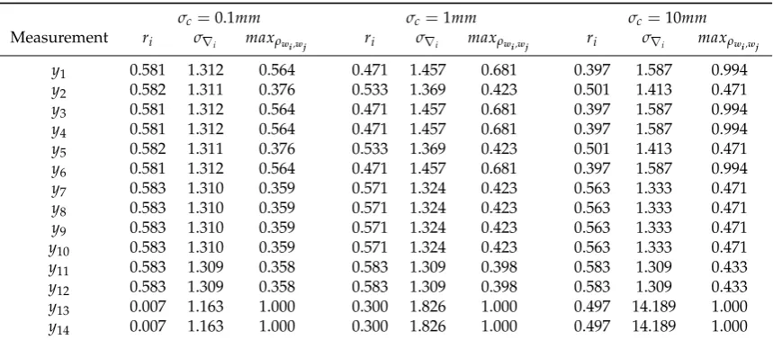
To analyse the constraints effects on theIDS, an example is taken from a geodetic levelling network with 12 height differences between the points. The equipment used to measure the level difference can be an electronic digital level. In that case, the levelling measurement system comprises of a special bar-coded staff (also called barcode rod) and a digital level (instrument). A digital level is basically a telescope that enables a horizontal line of sight. Digital levels consist of additional electronic image processing components to automatically read and analyse digital (bar coded) levelling staffs, where the graduation is replaced by a manufacturer dependent code pattern. Generally, the result is automatically stored in the data collector of the digital level. An example of a "digital level – bar-code staff" system is displayed in the Figure2. For more details about digital level see e.g. [81–84].
Figure 2.Example of adigital level – bar-code staff system [45].
The standard-deviation of the uncorrelated measurements were the same and taken equal to
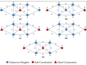
σ=1mm. The points are indicated as A to G. The eight network configuration are displayed in Figure 3(a, b, c, d, and e) and their details are given as follows:
1. Figure 3(a): Network with 1 hard constraint (i.e. network minimally constrained). Since the dimension of the network is 1D, the minimum information necessary to estimate the unknown heights is one. The height of G was fixed as control point (hard constraint), and 6 unknown heights (A,B,C,D,E,F) were minimally constrained. Therefore, the redundancy of the system (or overall degrees of freedom) wasr=n−rank(A) =n−u=12−6=6.
in that case wasr=12−5=7 with 5 unknown heights (B,C,E,F,G) over-constrained.
3. Figure3(c): Network with two extra hard constraints (i.e. three hard constraints).The heights A, D and G were taken as hard constraints. In that case, the redundancy of the system wasr=12−4=8. 4. Figure3(d): Network with two soft constraints (A and D). In that case, a standard-deviation larger than zero was assigned to both constraints (i.e.σc>0. In other words, A and D were processed
as being both observations and unknown parameters, i.e. A and D were pseudo-observations. Here, the both constraints were simultaneouslyrelaxedby considering their uncertainties 10 times worse than measurements (i.e. σc = 10×σ = 10mm); 10 times better than measurements (i.e. σc = 0.1mm); and their uncertainties equal to the measurements (σc = 1mm). In that case, the
redundancy of the system wasr=14−7=7.
5. Figure3(e): Network processed with A, D and G as pseudo-observations. Those three constraints were simultaneouslyrelaxedby considering their standard-deviations equal toσc=10mm(10 times
worse than measurements);σc=0.1mm(10 times better than measurements); andσc=1mm(the
same as the measurements). In that case, the redundancy of the system wasr=15−7=8.
y1 y2 y3 y4 y5 y6
y7 y8
y9
y10
B C
D E F G y12 y11 A y1 y2 y3 y4 y5 y6
y7 y8
y9
y10
A
B C
D E F G y12 y11 y1 y2 y3 y4 y5 y6
y7 y8
y9
y10
A
B C
D E F G y12 y11
(a) (b)
(c) (d)
(e)
Unknown Heights Soft Constraints Hard Constraints
y1 y2 y3 y4 y5 y6
y7 y8
y9
y10
A
B C
D E F G y12 y11 y1 y2 y3 y4 y5 y6
y7 y8
y9
y10
A
B C
D E F G y12 y11
Figure 3.Levelling Geodetic Network subject to different constraint scenarios.
y1+e1=hB−hA y2+e2=hC−hB y3+e3=hD−hC
.. .
y7+e7=hB−hG y8+e8=hC−hG
.. .
y11+e11=hB−hF y12+e12=hC−hE
(49)
The functional model (A) for the system of equations in49is given by:
A=
−1 1 0 0 0 0 0
0 −1 1 0 0 0 0
0 0 −1 1 0 0 0
0 0 0 −1 1 0 0
0 0 0 0 −1 1 0
1 0 0 0 0 −1 0
0 1 0 0 0 0 −1
0 0 1 0 0 0 −1
0 0 0 0 1 0 −1
0 0 0 0 0 1 −1
0 1 0 0 0 −1 0
0 0 1 0 −1 0 0
(50)
Note that the rank defect of the matrixAisu−rank(A) =7−6=1. In that case, there is needed to add at least one constraint in order to avoid rank deficiency of the matrixA. This is guaranteed when we take one height as known. For example, from the network in Figure3(a), we have added the height G as known (i.e. as a hard constraint). In that case, the constraint equation should be added into the system in49, i.e.:
y13=hGwithσy13 =0, (51)
noticing that because the standard deviation is zero, the observation is non-stochastic (hard constraint) and the residualey13=0. This can generate problems in the inversion of the covariance matrix of the
observationsQefor the calculation of the weight matrixW, because the weight for that constraint would be 10 =∞. In order to avoid that problem, we have eliminated the rank deficiency of matrix Aby removing the seventh column of matrix Ain50associated with the height G. Now, we have
u−rank(A) =6−6=0.
The constraint defines the geodetic datum, i.e. the S-system ([85],p.41). Another approach to solving the system of equations in2could be based on generalised (pseudo) inverses (see e.g. [86]).
The location of the constraints can be chosen in some circumstances, for example during the design stage of a geodetic network. For the special case of having a minimally constrained system, the location of the constraint will not influence thew-test statistics and the sensitivity indicators (MIB and MDB) [18]. However, more constraints than the minimum necessary to have a solution (i.e. extra constraints or redundant constraints) can change the least-squares residuals and hencew-test statistics and the minimal biases.
the two heights as hard constraints. For the case where these two heights (A and D) were taken as soft constraints, however, two observation equations were added to Equation49, i.e.:
y13+e13=hA, σy13 >0
y14+e14=hD, σy14>0
(52)
In the case of soft constraints in Equation52, two lines were added in matrixA. In other words, A and D were taken as pseudo-observations. In that case, the rank deficiency was also null (i.e.
u−rank(A) =7−7=0), the redundancy of the system wasr=n−rank(A) =n−u=7 and the matrixAwas given as follows:
A=
−1 1 0 0 0 0 0
0 −1 1 0 0 0 0
0 0 −1 1 0 0 0
0 0 0 −1 1 0 0
0 0 0 0 −1 1 0
1 0 0 0 0 −1 0
0 1 0 0 0 0 −1
0 0 1 0 0 0 −1
0 0 0 0 1 0 −1
0 0 0 0 0 1 −1
0 1 0 0 0 −1 0
0 0 1 0 −1 0 0
1 0 0 0 0 0 0
0 0 0 1 0 0 0
(53)
For this example of two soft constraints, and by considering the both soft constraints with standard-deviationσc =10mm, the symmetric and positive semi-definite covariance matrix of the
observations (Qe) was given as follows:
Qe=
1 0 0 · · · 0 0 0 1 0 · · · 0 0 0 0 1 · · · 0 0
..
. ... ... . .. ... ... 0 0 0 · · · 100 0 0 0 0 · · · 0 100
(54)
The last two rows and columns of the matrixQe in Equation54refer to the variances (σc2 = (10mm)2=100mm2) of the heights constraints A and D, respectively.
Similarly, matricesAandQewere constructed for the other cases studied here.
Although other measurements are able to identify an outlier for the case of having only one single soft constraint, the pseudo-observation (constraint) is not. In that case, the defect configuration is associated with the additional parameter in the constraint (i.e. the presence of an outlier in the constraint). In other words, an additional parameter on the soft constraint will not estimable. For example, if the height point G was taken as a soft constraint, the presence of an outlier in pseudo-observation G would lead to rank deficiency of matrix A, i.e. u−rank(A) = 8−7 = 1. Therefore, the case of having only one single soft constraint was not considered here.
4.2. Result of the Hard Constraint Effects on the Iterative Outlier Elimination Procedure
The correlation coefficient betweenw-test statistics (ρwi,wj) were computed for the three scenarios,
according to Equation(20). Table1provides that correlation for that network minimally constrained, Table2for that network over-constrained with two hard constraints and Table3for that network over-constrained with three hard constraints.
Table 1.Correlation matrix ofw-test statistics for the levelling network minimally constrained in Figure 3(a).
wy1 wy2 wy3 wy4 wy5 wy6 wy7 wy8 wy9 wy10 wy11 wy12
wy1 1.0 0.2 0.1 0.1 0.2 1.0 -0.2 0.0 0.0 0.2 -0.4 -0.1
wy2 1.0 0.2 0.2 0.3 0.2 0.5 -0.5 -0.2 0.2 0.3 -0.3
wy3 1.0 1.0 0.2 0.1 0.0 0.2 -0.2 0.0 0.1 0.4
wy4 1.0 0.2 0.1 0.0 0.2 -0.2 0.0 0.1 0.4
wy5 1.0 0.2 -0.2 0.2 0.5 -0.5 0.3 -0.3
wy6 1.0 -0.2 0.0 0.0 0.2 -0.4 -0.1
wy7 1.0 -0.3 -0.3 -0.4 -0.4 -0.1
wy8 1.0 -0.4 -0.3 -0.1 -0.4
wy9 1.0 -0.3 0.1 0.4
wy10 1.0 0.4 0.1
wy11 1.0 -0.1
wy12 1.00
Table 2.Correlation matrix ofw-test statistics for the levelling network with two hard constraints in Figure3(b).
wy1 wy2 wy3 wy4 wy5 wy6 wy7 wy8 wy9 wy10 wy11 wy12
wy1 1.0 0.4 0.4 -0.3 -0.1 0.4 -0.3 0.1 0.1 0.1 -0.4 -0.1
wy2 1.0 0.4 -0.1 0.1 -0.1 0.4 -0.4 -0.1 0.1 0.3 -0.3
wy3 1.0 0.4 -0.1 -0.3 -0.1 0.3 -0.1 -0.1 0.1 0.4
wy4 1.0 0.4 0.4 0.1 0.1 -0.3 0.1 0.1 0.4
wy5 1.0 0.4 -0.1 0.1 0.4 -0.4 0.3 -0.3
wy6 1.0 -0.1 -0.1 -0.1 0.3 -0.4 -0.1
wy7 1.0 -0.4 -0.3 -0.4 -0.4 -0.1
wy8 1.0 -0.4 -0.3 -0.1 -0.4
wy9 1.0 -0.4 0.1 0.4
wy10 1.0 0.4 0.1
wy11 1.0 -0.1
wy12 1.0
Table 3.Correlation matrix ofw-test statistics for the levelling network with three hard constraints in Figure3(c).
wy1 wy2 wy3 wy4 wy5 wy6 wy7 wy8 wy9 wy10 wy11 wy12
wy1 1.0 0.3 0.1 -0.1 -0.1 0.1 -0.4 -0.1 -0.1 -0.1 -0.3 -0.1
wy2 1.0 0.3 -0.1 0.1 -0.1 0.3 -0.3 -0.1 0.1 0.3 -0.3
wy3 1.0 0.1 -0.1 -0.1 0.1 0.4 0.1 0.1 0.1 0.3
wy4 1.0 0.3 0.1 -0.1 -0.1 -0.4 -0.1 0.1 0.3
wy5 1.0 0.3 -0.1 0.1 0.3 -0.3 0.3 -0.3
wy6 1.0 0.1 0.1 0.1 0.4 -0.3 -0.1
wy7 1.0 -0.1 -0.1 -0.1 -0.3 -0.1
wy8 1.0 -0.1 -0.1 -0.1 -0.3
wy9 1.0 -0.1 0.1 0.3
wy10 1.0 0.3 0.1
wy11 1.0 -0.1
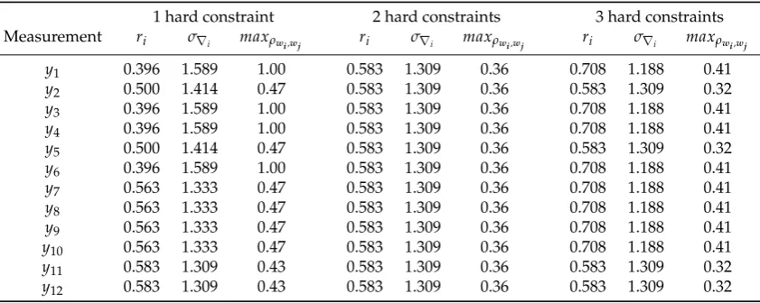
Table4gives the local redundancy (ri), the standard-deviation of the LS-estimated outlierσ∇i and
the maximum absolute correlation (maxρwi,wj) for each scenario of hard constraint set out of in this
study, i.e. Figure3(a,b and c).
Table 4.Local redundancy (ri), standard-deviation of the LS-estimated outlierσ∇iand the maximum
absolute correlation (maxρwi,wj) for each scenario of hard constraint.
1 hard constraint 2 hard constraints 3 hard constraints Measurement ri σ∇i maxρwi,wj ri σ∇i maxρwi,wj ri σ∇i maxρwi,wj
y1 0.396 1.589 1.00 0.583 1.309 0.36 0.708 1.188 0.41
y2 0.500 1.414 0.47 0.583 1.309 0.36 0.583 1.309 0.32
y3 0.396 1.589 1.00 0.583 1.309 0.36 0.708 1.188 0.41
y4 0.396 1.589 1.00 0.583 1.309 0.36 0.708 1.188 0.41
y5 0.500 1.414 0.47 0.583 1.309 0.36 0.583 1.309 0.32
y6 0.396 1.589 1.00 0.583 1.309 0.36 0.708 1.188 0.41
y7 0.563 1.333 0.47 0.583 1.309 0.36 0.708 1.188 0.41
y8 0.563 1.333 0.47 0.583 1.309 0.36 0.708 1.188 0.41
y9 0.563 1.333 0.47 0.583 1.309 0.36 0.708 1.188 0.41
y10 0.563 1.333 0.47 0.583 1.309 0.36 0.708 1.188 0.41
y11 0.583 1.309 0.43 0.583 1.309 0.36 0.583 1.309 0.32
y12 0.583 1.309 0.43 0.583 1.309 0.36 0.583 1.309 0.32
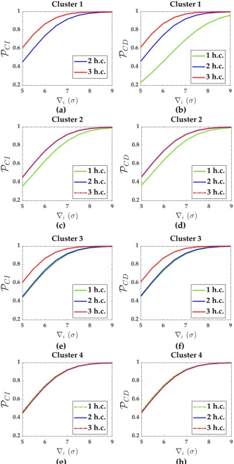
Here, the twelve levelling measurements were clustered into four clusters. The clustering was defined according to the local redundancy (ri) and the maximum absolute correlation (maxρwi,wj) in Table4. This is the first time that a clustering technique based on the similarity of local redundancy and the maximum absolute correlation betweenw-test statistics is applied to a problem of geodetic networks. Similarly, this has been done in [45]. The four cluster were defined as follows:
• Cluster 1:y1,y3,y4andy6.
• Cluster 2:y2andy5. • Cluster 3:y7,y8,y9andy10. • Cluster 4:y11andy12.
The probability levels associated withIDSwere averaged for each of these clusters. Here, we compute the probability levels of theIDSbased on the procedure in Section (3) [45]. The critical values were ˆ
k = 3.89, ˆk = 3.93 and ˆk = 3.93 for 1 hard constraint, 2 hard constraints and 3 hard constraints, respectively. These critical values were found forα0 =0.001 according to the procedure described in
Appendix??. The probability of correct identification (PCI) and correct detection (PCD =1− PMD)
(c) (d)
(e) (f)
(g) (h)
(a) (b)
Figure 4.Probability of correct identification (PCI) and Probability of correct detection (PCD) for the case of hard constraints and forα0=0.001: Cluster 1(a,b), Cluster 2(c,d), Cluster 3(e,f) and Cluster
The outlier magnitude were defined from|5σ|to|9σ|. The outlier of|5σ|was chosen because it
is approximately the lowestMDB0(i)of the network when a single hypothesis testing is in play, as
can be seen in Equation (14) or Equation (16). ThatMDB0(i)of|5σ|was computed for significance
level ofα0=0.001 and a power of the testγ0=0.8. This strategy reduces the search space for a MIB
(Minimal Identifiable Bias), because we will always have the following inequalityMIB≥MDB0(i)
[47,55]. Remember that theIDSprocedure is an example of multiple hypothesis testing (see2). The sensitivity indicators MDB and MIB forIDSwere also computed according to Equation (33) and (34), respectively. The success rate for outlier detection and outlier identification were taken as being ˜PCD =P˜CI =0.8, respectively. Table5provides the values of MDB and MIB for that case of hard constraints.
Table 5.MDB and MIB for the case of hard constraints based onα0=0.001 and ˜PCD=P˜CI=0.8.
1 hard constraint 2 hard constraints 3 hard constraints Cluster MDB (σ) MIB (σ) MDB (σ) MIB (σ) MDB (σ) MIB (σ)
1 7.5 - 6.3 6.3 5.7 5.7
2 6.7 6.8 6.3 6.4 6.3 6.4
3 6.4 6.4 6.3 6.3 5.8 5.8
4 6.4 6.4 6.4 6.4 6.4 6.4
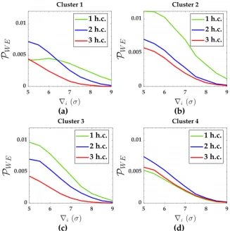
Figure5shows the probability of wrong exclusion (PWE). The over-identification cases (Pover+
andPover−) were smaller than 0.001 (i.e. they were practically null). There were not statistical overlap
(Pol) for clusters 2, 3 and 4. We will discuss more about statistical overlap (Pol) later.
(c) (d)
(a) (b)
Figure 5.Probability of wrong exclusion (PWE) for the case of hard constraints and forα0 =0.001:
4.3. Result of the Soft Constraint Effects on the Iterative Outlier Elimination Procedure
The both configuration in Figure3(d) and Figure3(e) were analysed in terms of soft constraints. In that case, the critical values were ˆk = 3.95, ˆk= 3.95 and ˆk = 3.92 for two soft constraints with
σc=0.1mm,σc=1mmandσc=10mm, respectively. In the case of three soft constraints, the critical
values found were ˆk = 3.99, ˆk = 3.99 and ˆk = 3.96 forσc = 0.1mm, σc = 1mmandσc = 10mm,
respectively. All these critical values were computed forα0=0.001.
The correlation coefficient betweenw-test statistics (ρwi,wj) are displayed in Table6, Table 7
and Table8for two soft constraints with standard-deviation 10 times larger than measurements (i.e. σc = 10×σ =10mm); 10 times better than measurements (i.e. σc = 0.1mm); and equal to the
measurements (σc=1mm), respectively.
Table 6.Correlation matrix ofw-test statistics for the levelling network with two soft constraints with
σc=10mmin Figure3(d).
wy1 wy2 wy3 wy4 wy5 wy6 wy7 wy8 wy9 wy10 wy11 wy12 wy13 wy14
wy1 1.0 0.2 0.1 0.1 0.2 1.0 -0.2 0.0 0.0 0.2 -0.4 -0.1 0.06 -0.1
wy2 1.0 0.2 0.2 0.3 0.2 0.5 -0.5 -0.2 0.2 0.3 -0.3 0.03 0.0
wy3 1.0 1.0 0.2 0.1 0.0 0.2 -0.2 0.0 0.1 0.4 0.1 -0.1
wy4 1.0 0.2 0.1 0.0 0.2 -0.2 0.0 0.1 0.4 -0.1 0.1
wy5 1.0 0.2 -0.2 0.2 0.5 -0.5 0.3 -0.3 0.0 0.0
wy6 1.0 -0.2 0.0 0.0 0.2 -0.4 -0.1 -0.1 0.1
wy7 1.0 -0.3 -0.3 -0.4 -0.4 -0.1 0.0 0.0
wy8 1.0 -0.4 -0.3 -0.1 -0.4 0.0 0.0
wy9 1.0 -0.3 0.1 0.4 0.0 0.0
wy10 1.0 0.4 0.1 0.0 0.0
wy11 1.0 -0.1 0.0 0.0
wy12 1.0 0.0 0.0
wy13 1.0 -1.0
wy14 1.0
Table 7.Correlation matrix ofw-test statistics for the levelling network with two soft constraints with
σc=0.1mmin Figure3(d).
wy1 wy2 wy3 wy4 wy5 wy6 wy7 wy8 wy9 wy10 wy11 wy12 wy13 wy14
wy1 1.0 0.4 0.4 -0.3 -0.1 0.4 -0.3 0.1 0.1 0.1 -0.4 -0.1 0.6 -0.6
wy2 1.0 0.4 -0.1 0.2 -0.1 0.4 -0.4 -0.1 0.1 0.3 -0.3 0.4 -0.4
wy3 1.0 0.4 -0.1 -0.3 -0.1 0.3 -0.1 -0.1 0.1 0.4 0.6 -0.6
wy4 1.0 0.4 0.4 0.1 0.1 -0.3 0.1 0.1 0.4 -0.6 0.6
wy5 1.0 0.4 -0.1 0.1 0.4 -0.4 0.3 -0.3 -0.4 0.4
wy6 1.0 -0.1 -0.1 -0.1 0.3 -0.4 -0.1 -0.6 0.6
wy7 1.0 -0.4 -0.3 -0.4 -0.4 -0.1 -0.2 0.2
wy8 1.0 -0.4 -0.3 -0.1 -0.4 0.2 -0.2
wy9 1.0 -0.4 0.1 0.4 0.2 -0.2
wy10 1.0 0.4 0.1 -0.2 0.2
wy11 1.0 -0.1 0.0 0.0
wy12 1.0 0.0 0.0
wy13 1.0 -1.0
Table 8.Correlation matrix ofw-test statistics for the levelling network with two soft constraints with
σc=1mmin Figure3(d).
wy1 wy2 wy3 wy4 wy5 wy6 wy7 wy8 wy9 wy10 wy11 wy12 wy13 wy14
wy1 1.0 0.3 0.2 -0.1 0.1 0.7 -0.3 0.0 0.1 0.2 -0.4 -0.1 0.4 -0.4
wy2 1.0 0.3 0.1 0.3 0.1 0.4 -0.4 -0.1 0.1 0.3 -0.3 0.3 -0.3
wy3 1.0 0.7 0.1 -0.1 0.0 0.3 -0.2 -0.1 0.1 0.4 0.4 -0.4
wy4 1.0 0.3 0.2 0.1 0.2 -0.3 0.0 0.1 0.4 -0.4 0.4
wy5 1.0 0.3 -0.1 0.1 0.4 -0.4 0.3 -0.3 -0.3 0.3
wy6 1.0 -0.2 -0.1 0.0 0.3 -0.4 -0.1 -0.4 0.4
wy7 1.0 -0.3 -0.3 -0.4 -0.4 -0.1 -0.1 0.1
wy8 1.0 -0.4 -0.3 -0.1 -0.4 0.1 -0.1
wy9 1.0 -0.3 0.1 0.4 0.1 -0.1
wy10 1.0 0.4 0.1 -0.1 0.1
wy11 1.0 -0.1 0.0 0.0
wy12 1.0 0.0 0.0
wy13 1.0 -1.0
wy14 1.0
Table9gives the local redundancy (ri), the standard-deviation of the LS-estimated outlierσ∇i and
the maximum absolute correlation (maxρwi,wj) for the scenarios of two constraints.
Table 9. Local redundancy (ri), standard-deviation of the LS-estimated outlierσ∇i(mm) and the
maximum absolute correlation (maxρwi,wj) for each scenario of two soft constraints.
σc=0.1mm σc=1mm σc=10mm
Measurement ri σ∇i maxρwi,wj ri σ∇i maxρwi,wj ri σ∇i maxρwi,wj
y1 0.581 1.312 0.564 0.471 1.457 0.681 0.397 1.587 0.994 y2 0.582 1.311 0.376 0.533 1.369 0.423 0.501 1.413 0.471 y3 0.581 1.312 0.564 0.471 1.457 0.681 0.397 1.587 0.994 y4 0.581 1.312 0.564 0.471 1.457 0.681 0.397 1.587 0.994 y5 0.582 1.311 0.376 0.533 1.369 0.423 0.501 1.413 0.471 y6 0.581 1.312 0.564 0.471 1.457 0.681 0.397 1.587 0.994 y7 0.583 1.310 0.359 0.571 1.324 0.423 0.563 1.333 0.471 y8 0.583 1.310 0.359 0.571 1.324 0.423 0.563 1.333 0.471 y9 0.583 1.310 0.359 0.571 1.324 0.423 0.563 1.333 0.471 y10 0.583 1.310 0.359 0.571 1.324 0.423 0.563 1.333 0.471 y11 0.583 1.309 0.358 0.583 1.309 0.398 0.583 1.309 0.433 y12 0.583 1.309 0.358 0.583 1.309 0.398 0.583 1.309 0.433 y13 0.007 1.163 1.000 0.300 1.826 1.000 0.497 14.189 1.000 y14 0.007 1.163 1.000 0.300 1.826 1.000 0.497 14.189 1.000
From Table9, five clusters were defined for each case of two soft constraints, i.e. for the case where heights A and D were given as soft constraints in Figure3(d), as follows:
• Cluster 1:y1,y3,y4andy6.
• Cluster 2:y2andy5. • Cluster 3:y7,y8,y9andy10. • Cluster 4:y11andy12. • Cluster 5:y13andy14.
The probabilities of correct identification (PCI) and correct detection (PCD) for the measurements
(c) (d)
(e) (f)
(g) (h)
(a) (b)
Figure 6.Probability of correct identification (PCI) and Probability of correct detection (PCD) for the measurements subject to the scenarios of two soft constraints forα0=0.001: Cluster 1(a,b), Cluster
Note that the Cluster 5 is associated with the two soft constraints (i.e.y13andy14). The probability of correct identification (PCI) for these both soft constraints were null. However, the probability of correct detection were not. Figure7shows the probability of correct detection (PCD) for these two soft
constraints (i.e. heights A and D).
Figure 7.Probability of correct detectionPCDfor the two soft constraints (Cluster 5: heights A and D) and forα0=0.001.
The probability of wrong exclusionPWEfor the measurements (Cluster 1 to Cluster 4) subject to
the scenarios of two soft constraints (heights A and D) are displayed in Figure8. Figure9gives the the probability of wrong exclusionPWEfor that two constraints (i.e. heights A and D).
(c) (d)
(a) (b)
Figure 9.Probability of wrong exclusionPWEfor the two soft constraints (Cluster 5: heights A and D) and forα0=0.001.
The over-identification cases (Pover+andPover−) and the statistical overlap (Pol) were practically
null for that case.
The sensitivity indicators (MDB and MIB) for each scenario of two soft constraints are displayed in Table10.
Table 10.MDB and MIB for the case of two soft constraints based onα0=0.001 and ˜PCD=P˜CI=0.8.
σc=10mm σc=1mm σc=0.1mm
Cluster MDB (σ) MIB (σ) MDB (σ) MIB (σ) MDB (σ) MIB (σ)
1 7.5 25 7 7.1 6.3 6.3
2 6.8 6.8 6.6 6.6 6.3 6.3
3 6.4 6.4 6.4 6.4 6.3 6.3
4 6.3 6.3 6.3 6.3 6.3 6.3
5 6.8 - 8.8 - 57
-As with the case of two soft constraints, Tables11,12and13show the correlations (ρwi,wj) for the
case where there were three soft constraints, i.e. for the network configuration in Figure3(e).
Table 11. Correlation matrix ofw-test statistics for the levelling network with three soft constraints withσc=10mmin Figure3(e).
wy1 wy2 wy3 wy4 wy5 wy6 wy7 wy8 wy9 wy10 wy11 wy12 wy13 wy14 wy15
wy1 1.0 0.2 0.1 0.1 0.2 1.0 -0.2 0.0 0.0 0.2 -0.4 -0.1 0.1 0.0 0.0
wy2 1.0 0.2 0.2 0.3 0.2 0.5 -0.5 -0.2 0.2 0.3 -0.3 0.0 0.0 0.0
wy3 1.0 1.0 0.2 0.1 0.0 0.2 -0.2 0.0 0.1 0.4 0.0 -0.1 0.0
wy4 1.0 0.2 0.1 0.0 0.2 -0.2 0.0 0.1 0.4 0.0 0.1 0.0
wy5 1.0 0.2 -0.2 0.2 0.5 -0.5 0.3 -0.3 0.0 0.0 0.0
wy6 1.0 -0.2 0.0 0.0 0.2 -0.4 -0.1 -0.1 0.0 0.0
wy7 1.0 -0.3 -0.3 -0.4 -0.4 -0.1 0.0 0.0 0.0
wy8 1.0 -0.4 -0.3 -0.1 -0.4 0.0 0.0 0.0
wy9 1.0 -0.3 0.1 0.4 0.0 0.0 0.0
wy10 1.0 0.4 0.1 0.0 0.0 0.0
wy11 1.0 -0.1 0.0 0.0 0.0
wy12 1.0 0.0 0.0 0.0
wy13 1.0 -0.5 -0.5
wy14 1.0 -0.5
Table 12. Correlation matrix ofw-test statistics for the levelling network with three soft constraints withσc=0.1mmin Figure3(e).
wy1 wy2 wy3 wy4 wy5 wy6 wy7 wy8 wy9 wy10 wy11 wy12 wy13 wy14 wy15
wy1 1.0 0.3 0.1 -0.1 -0.1 0.1 -0.4 -0.1 -0.1 -0.1 -0.3 -0.1 0.7 -0.1 -0.4
wy2 1.0 0.3 -0.1 0.1 -0.1 0.3 -0.3 -0.1 0.1 0.3 -0.3 0.3 -0.3 0.0
wy3 1.0 0.1 -0.1 -0.1 0.1 0.4 0.1 0.1 0.1 0.3 0.1 -0.7 0.4
wy4 1.0 0.3 0.1 -0.1 -0.1 -0.4 -0.1 0.1 0.3 -0.1 0.7 -0.4
wy5 1.0 0.3 -0.1 0.1 0.3 -0.3 0.3 -0.3 -0.3 0.3 0.0
wy6 1.0 0.1 0.1 0.1 0.4 -0.3 -0.1 -0.7 0.1 0.4
wy7 1.0 -0.1 -0.1 -0.1 -0.3 -0.1 -0.4 -0.1 0.4
wy8 1.0 -0.1 -0.1 -0.1 -0.3 -0.1 -0.4 0.4
wy9 1.0 -0.1 0.1 0.3 -0.1 -0.4 0.4
wy10 1.0 0.3 0.1 -0.4 -0.1 0.4
wy11 1.0 -0.1 0.0 0.0 0.0
wy12 1.0 0.0 0.0 0.0
wy13 1.0 -0.2 -0.6
wy14 1.0 -0.6
wy15 1.0
Table 13. Correlation matrix ofw-test statistics for the levelling network with three soft constraints withσc=1mmin Figure3(e).
wy1 wy2 wy3 wy4 wy5 wy6 wy7 wy8 wy9 wy10 wy11 wy12 wy13 wy14 wy15
wy1 1.0 0.3 0.1 0.0 0.1 0.6 -0.3 0.0 0.0 0.1 -0.4 -0.1 0.5 -0.2 -0.2
wy2 1.0 0.3 0.1 0.3 0.1 0.4 -0.4 -0.1 0.1 0.3 -0.3 0.2 -0.2 0.0
wy3 1.0 0.6 0.1 0.0 0.0 0.3 -0.1 0.0 0.1 0.4 0.2 -0.5 0.2
wy4 1.0 0.3 0.1 0.0 0.1 -0.3 0.0 0.1 0.4 -0.2 0.5 -0.2
wy5 1.0 0.3 -0.1 0.1 0.4 -0.4 0.3 -0.3 -0.2 0.2 0.0
wy6 1.0 -0.1 0.0 0.0 0.3 -0.4 -0.1 -0.5 0.2 0.2
wy7 1.0 -0.3 -0.2 -0.3 -0.4 -0.1 -0.2 0.0 0.2
wy8 1.0 -0.3 -0.2 -0.1 -0.4 0.0 -0.2 0.2
wy9 1.0 -0.3 0.1 0.4 0.0 -0.2 0.2
wy10 1.0 0.4 0.1 -0.2 0.0 0.2
wy11 1.0 -0.1 0.0 0.0 0.0
wy12 1.0 0.0 0.0 0.0
wy13 1.0 -0.4 -0.5
wy14 1.0 -0.5
wy15 1.0
Table 14. Local redundancy (ri), standard-deviation of the LS-estimated outlierσ∇i(mm) and the
maximum absolute correlation (maxρwi,wj) for each scenario of three soft constraints.
σc=0.1mm σc=1mm σc=10mm
Measurement ri σ∇i maxρwi,wj ri σ∇i maxρwi,wj ri σ∇i maxρwi,wj
y1 0.702 1.194 0.660 0.502 1.411 0.577 0.398 1.586 0.992
y2 0.582 1.311 0.326 0.533 1.369 0.412 0.501 1.413 0.470
y3 0.702 1.194 0.660 0.502 1.411 0.577 0.398 1.586 0.992
y4 0.702 1.194 0.660 0.502 1.411 0.577 0.398 1.586 0.992
y5 0.582 1.311 0.326 0.533 1.369 0.412 0.501 1.413 0.470
y6 0.702 1.194 0.660 0.502 1.411 0.577 0.398 1.586 0.992
y7 0.704 1.192 0.415 0.602 1.289 0.412 0.563 1.333 0.470
y8 0.704 1.192 0.415 0.602 1.289 0.412 0.563 1.333 0.470
y9 0.704 1.192 0.415 0.602 1.289 0.412 0.563 1.333 0.470
y10 0.704 1.192 0.415 0.602 1.289 0.412 0.563 1.333 0.470
y11 0.583 1.309 0.326 0.583 1.309 0.385 0.583 1.309 0.433
y12 0.583 1.309 0.326 0.583 1.309 0.385 0.583 1.309 0.433
y13 0.012 0.904 0.660 0.425 1.534 0.542 0.663 12.283 0.501
y14 0.012 0.904 0.660 0.425 1.534 0.542 0.663 12.283 0.501
y15 0.019 0.718 0.63 0.5 1.414 0.542 0.665 12.268 0.501
The probabilities of correct identification (PCI) and correct detectionPCDfor the measurements
![Figure 1. Flowchart of the algorithm to compute the probability levels of Iterative Data Snooping (IDS)for each measurement in the presence of an outlier [45].](https://thumb-us.123doks.com/thumbv2/123dok_us/7918933.1314896/11.595.80.515.83.561/figure-flowchart-algorithm-probability-iterative-snooping-measurement-presence.webp)
![Figure 2. Example of a digital level – bar-code staff system [45].](https://thumb-us.123doks.com/thumbv2/123dok_us/7918933.1314896/14.595.171.426.370.586/figure-example-digital-level-bar-code-staff-system.webp)