Historical collaborative geocoding
Rémi Cura1,4,† ID, Bertrand Dumenieu3,4,†ID, Nathalie Abadie2, Benoit Costes2, Julien Perret 2,3,4ID, Maurizio Gribaudi3,4
1 IGN; [email protected]
2 IGN; [email protected]
3 EHESS; [email protected]
4 GeoHistoricalData; [email protected]
* Correspondence: [email protected]
† These authors contributed equally to this work.
Abstract: The latest developments in digital humanities have increasingly enabled the construction
1
of large data sets which can easily be accessed and used. These data sets often contain indirect
2
localisation information, such as historical addresses. Historical geocoding is the process of
3
transforming the indirect localisation information to direct localisation that can be placed on a
4
map, which enables spatial analysis and cross-referencing. Many efficient geocoders exist for current
5
addresses, but they do not deal with temporal information and are usually based on a strict hierarchy
6
(country, city, street, house number, etc.) that is hard, if not impossible, to use with historical data.
7
Indeed, historical data are full of uncertainties (temporal, textual, positional accuracy, confidence
8
in historical sources) that can not be ignored or entirely resolved. We propose an open source,
9
open data, extensible solution for geocoding that is based on gazetteers composed of geohistorical
10
objects extracted from historical topographical maps. Once the gazetteers are available, geocoding an
11
historical address is a matter of finding the geohistorical object in the gazetteers that is the best match
12
to the historical address searched by the user. The matching criteria are customisable and include
13
several dimensions (fuzzy string, fuzzy temporal, level of detail, positional accuracy). As the goal
14
is to facilitate historical work, we also propose web-based user interfaces that help geocode (one
15
address or batch mode) and display over current or historical topographical maps, so that geocoding
16
results can be checked and collaboratively edited. The system has been tested on the city of Paris,
17
France, for the 19th and the 20th centuries. It shows high response rates and is fast enough to be used
18
interactively.
19
Keywords: Historical dataset; geocoding; localisation; geohistorical objects; database; GIS;
20
collaborative; citizen science; crowd-sourced; digital humanities
21
1. Introduction
22
1.1. Context
23
In historical sciences, cartography and spatial analysis are extensively used to reveal the spatial
24
organisations that hide within data with textual indirect spatial references like placenames or postal
25
addresses. Mapping such data requires each item to be geocoded,i.e. assigned with coordinates
26
on the Earth surface by matching the indirect spatial reference with entities identified in a reference
27
geographical datasource (e.g.a topographic map georeferenced in a well-known coordinate reference
28
system) [1]. Problems emerge when such spatial references are obsolete due to the temporal gap
29
between the data to be geocoded and the reference datasource: locating the London Crystal Palace
30
(destroyed by fire in 1936) on a today map would be rather tricky. Worse still, it might create ambiguities
31
and possibly lead to erroneous geocoding, as the Crystal Palace refers nowadays to a South London
32
residential area. Whereas manual geocoding can deal with such cases, the constantly growing volume
33
of historical data, which results from the multiplication of initiatives in the digital humanities, calls for
34
automatic approaches. Despite the existence of highly efficient (atemporal) geocoding tools and API, a
35
truly historical geocoder is still at stake [2,3].
36
1.2. Related work
37
Geocoding is an inevitable step in any spatially-based study with considerable bodies of data,
38
which makes it a critical process in various contexts: public health, catastrophe risk management,
39
marketing, social sciences, etc. Many geocoding web services have been developed to fulfil this need,
40
originating from private initiatives (Google Geocoding API, Mapzen1), public agencies (the French
41
National Address Gazetteer2) or from the open-source community (OSM Nominatim3, Gisgraphy4).
42
These services can be characterized in terms of their three main components [1,4]: input/output data,
43
reference dataset and processing algorithm. Theinputis the textual description the user wants to
44
refine into coordinates (e.g."13 rue du temple, Paris, France"). Thereference datasetcontains geographic
45
features associated with textual descriptions of addresses. Theprocessing algorithmconsists in finding
46
the best match between the latter and the former input description. Finally, the output usually contains
47
a geographical feature and its similarity score (perfect match or approximate for instance).
48
These tools answer millions of geocoding queries each day with great success. Indeed, the
49
quality of geocoding services can be estimated via two very important criteria [5]. The first is the
50
database quality: how complete and up to date is the reference database? The second is the results
51
characterization: how spatially accurate is each result and what is its associated confidence?
52
Despite their quality, such geocoding approaches can not be used for (geo)historical data for
53
three main reasons. The first is that existing geocoding services do not take into account the temporal
54
aspect of the query or the dataset they rely on. Indeed, they usually rely on current data, such as
55
OpenStreetMap5data, continuously updated. As such, they implicitly work on a valid time that is the
56
present (or possibly the interval between the beginning of the database construction and the present
57
time). The second reason is that they rely on an exhaustive, strongly hierarchical database whose
58
accuracy can be checked against ground truth (i.e.there is always a way to check the actual localization
59
of an address). Unfortunately, historical data are not easily verifiable: one has to check them with
60
difference available (geo)historical sources (possibly incomplete and conflicting) and, often, making
61
assumptions or hypotheses. Such hypotheses are in their turn continuously challenged and updated
62
by new discoveries, and there is no way to give a truly definitive answer. Indeed, primary sources
63
may also be wrong or misleading. The third reason is that historical sources available to construct a
64
gazetteer are sparse (both spatially and temporally), heterogeneous, and complex. We believe that
65
all these specificities call for a dedicated approach. Similar observations have already been made
66
in the context of archival data by the UK National Archives for instance [6]. Large historical event
67
gazeteers already exist [7] and provide an important basis for the construction of the reference dataset.
68
Nevertheless, we found few related articles [2,8], and for all of them geocoding was not a focus.
69
We could not find an historical geocoding approach that considers the characterization of
70
geocoding results. Yet, this aspect is essential for historical geocoding because of the very unprecise
71
and sparse nature of geohistorical data. Indeed, geocoding results have to be validated and/or edited
72
manually. Considering the large amount of addresses (>100000f orParis) and the potential complexity
73
of the task, this is clearly a lot of work. Fortunately, several projects such asOpenStreetMaphave lead the
74
way for what is usually calledVolonteered Geographical Information(VGI) [9] ofcrowdsourcing geospatial
75
data[10]. This approach consists in using a collaborative approach to solve the problem collectively,
76
usually by implying citizens in the process. As suggested in a recent typology of participation in
77
1 mapzen.com
2 adresse.data.gouv.fr/api/
3 nominatim.openstreetmap.org
4 gisgraphy.com
citizen science and VGI [11], different levels of participation can be defined. These levels go from
78
“crowdsourcing”, where the cognitive demand is minimal, to “extreme citizen science” or “collaborative
79
science”, where citizens are involved in all stages of the research (problem definition, data collection
80
and analysis). In the rest of this article, we propose a collaborative historical geocoding approach
81
that opens a way for a simpler participation of citizens in geohistorical research (thanks to dedicated
82
interactive tools), but also for a more collaborative geohistorical science (thanks to a reproducible
83
research approach [12–15], open source tools and open data).
84
1.3. Approach and contributions
85
In this article, we focus on the historical geocoding problem. Following the classical approach, we
86
will present in particular the construction of a geohistorical database and the development of matching
87
(data linkage) methods that fully use the temporal aspects of the geohistorical data and the input query.
88
The main contributions of this article consist in (1) a formalisation of the historical geocoding problem,
89
(2) a minimal model of geohistorical objects that can be easily re-used and extended, (3) an open source
90
geocoding tool that is powerful, easy to use and can be extended with any geohistorical data, (4) a
91
graphical tool to control and edit the geocoding results, which can then optionally be used to enrich
92
the geohistorical database, (5) qualifications of geocoding results in term of textual, spatial, temporal
93
aspects.
94
2. Approach overview
95
Historical topographical maps
Build gazetteers of geohistorical objects
geohistorical_object_model
Gazetteers
name date s.
10 place Vendome 10 Place Vendome 12 place Vendome 10 Place Vendôme
1825-37 1887-89 1825-37 2015-16
27 28 42 43
...
geom
Point(1... Line((2... Poly(((... Point(2...
"10 place Vendfme, Paris"; 1850
adresse/date to geocode
Collaborative editing
...
find best matching
geohistorical objects
web UI
Figure 1. Gazetteers of geohistorical objects are created based on information extracted from georeferenced historical maps. Geocoding an historical address is then finding the best matching object based on a customised function (semantic, temporal aspect, spatial precision, etc.). Results can be displayed through a dedicated web interface for collaborative editing.
Based on historical sources and historical topographical maps, we extract geographic features
96
that are gathered into gazetteers. These (geo) historical feature are modeled in a generic way into a
97
Relational Database Management System (RDBMS). Geocoding an historical address is then finding
98
the geohistorical object in the gazetteer that best match this historical address, thus may be done by
99
means of distances that can be customised by the user. Lastly the results can be displayed via a web
100
mapping interface over current or historical topographical maps, and further checked and edited
101
collaboratively. Figure1illustrates this approach.
102
2.1. Building a geohistorical gazetteer: Extracting geohistorical objects from historical topographical maps
103
The starting point to build gazetteers is information extracted from historical topographical maps.
104
The first part of extraction is to digitize the maps and georeferencing the map in a defined coordinate
105
reference system. This maps are historical sources, and as such an historical analysis is performed to
106
estimated the probable valid time (temporalization), positional accuracy, completeness, confidence,
107
relation to other historical maps, etc. The whole process is carefully designed and explained in detail
in [16]. Then geohistorical objects are extracted from the referenced historical maps, manually (in a
109
collaborative way), or with the help of computer vision techniques.
110
2.1.1. General consideration about building a spatio-temporal database
111
Extracting information from topographic historical maps amounts to building a spatio-temporal
112
database. There are several approaches to do so, and we stress that we do not attempt to create a
113
continuous spatio-temporal database. Instead, we store representations of the same space at multiple
114
moments in history, the well-known snapshot model [17]. The main advantage is that for a given
115
moment in time we can have several conflicting snapshots coexisting. This is essential, as solving the
116
conflict may not be possible, and reporting these several conflicting geocoding results to historians
117
may help appreciate these results. The drawbacks of this model,i.e.information redundancy and its
118
inability to store the changes themselves, can be overcome during the geocoding process.
119
2.1.2. Historical topographic maps as geohistorical sources
120
In our approach, we focus on historical topographic maps as the main sources for two main
121
reasons:
122
• the way they portray spatial information is close to today topographic mapping, making the
123
integration of the information they convey in a Geographical Information System (GIS) easy;
124
• the main goal of topographic maps is to provide a reliable depiction of the shape and location of
125
geographical features.
126
Although this choice seriously reduces the number of possible sources and therefore lessens the
127
quantity of accessible spatial information, it aims at efficiency. Indeed, topographic maps are a
128
good compromise between their reliability, the quantity of spatial information they contain and the
129
complexity of extracting information.
130
We create a snapshot for each historical topographic map by relying on three steps:
131
1. georeferencing the map in a well-defined coordinate reference system supported by common
132
GIS tools,
133
2. assigning the map avalid time,
134
3. extracting geographical features from the map.
135
2.1.3. Georeferencing topographic historical maps
136
We have to establish a correspondence between each pixel of the historical maps and geographical
137
coordinates. To do so, we first choose a common spatial reference system (SRS). Then we identify
138
common geographic features between historical maps and current maps: so-called ground control
139
points (GCP). Last, we compute a warping transform that will respect at best the matching points.
140
Finding GCPs between current maps and historical maps can be increasingly difficult as we go back in
141
time, because there are less and less perenial GCPs. Consider for instance the city of Paris, where the
142
French Revolution and its consequences combined with the 19thcentury transformations (including
143
the so-called Haussmannian transformations) resulted in massive changes in the shape of the city. To
144
this end, we can start by georeferencinge.g. 20thmaps to current maps, then georeferencee.g. 19th
145
maps to 20thmaps, and so on for even older maps.
146
Common spatial reference system (SRS)
147
The choice of a SRS is not easy, as each SRS induces projection errors that depend on the
148
covered area. Whatever the choice of SRS, it is essential that the implied accuracy is well-known and
149
documented in order to qualify the absolute accuracy of each geo-referenced map. We restrain ourselfs
150
to SRS using meters as base units (opposed to SRS using degrees), as they are much closer in nature to
151
those used in historical topographical maps.
Selection of ground control points
153
The identification of pairs of GCPs is a critical step because the number, distribution and quality
154
(i.e. positional accuracy, reliability, confidence) of the points strongly influence the quality of the
155
georeferencing. While the quality of the selected points depends on each map, a simple rule of thumbs
156
is to select, as much as possible, homogeneously distributed points to go further [18]. Three parameters
157
have to be considered: the geometric type of the features carying the ground control points, their
158
nature and the method used to identify them. Usually, features chosen as ground control points are
159
represented by 2D points; lines or surfaces may also be used, and possibiliy even curves [19].
160
On historical maps, the positionnal accuracy of mapping themes can vary greatly either due to
161
the purpose of the map, or the mapmaking process itself. Optionally, one can rely on geodetic features
162
drawn on the map such as meridian or parallels provided one can fully characterised the geodetic
163
characteristics of these lines.
164
The actual identification of GCPs can be achieved by automatic or manual processes. Automatic
165
approaches are notably used for historical aerial photographs, where feature detection and matching
166
algorithms are well fitted [20]. Common GIS tools offer georeferencing softwares allowing to manually
167
select pairs ofground control pointsidentified in both the input and the reference maps. Such tools are
168
often used for historical maps georeferencing because: (1) they are easy to utilize and (2) they allow
169
historians to control the quality and reliability of the identified points using co-visualization between
170
both maps.
171
Choosing a geometric transformation model
172
Once an acceptable set of paired features has been identified, the last step is to compute the
173
transformation from the input map to the reference. Several transformation models have been
174
proposed: global transforms (affine, projective), global with local adaptations (polynomial-based) and
175
local transforms (rubbersheeting, Thin Plate Spline, kernel-based approaches, etc.). Studies have been
176
conducted to assess the relevance of these transformation for historical maps [18,21,22]. They show
177
that choosing a model is mostly a matter of compromise between the final spatial matching between
178
the feature pairs (i.e.the expected residual error) and the acceptable distortion of the map regarding
179
its legibility. Exact or near-perfect matching between features can be achieved with local transforms
180
and high order polynomials, whereas the internal structure of the map is most preserved by global
181
transformations. Low order polynomials offer a compromise between both constraints.
182
2.1.4. Temporalization: locating geohistorical sources in time
183
Georeferencing is a way of locating multiple maps in the same reference space. Similarly,
184
temporalization is the process of locating each geohistorical source in time. When building
185
spatio-temporal snapshots from historical maps, the key problem is to determine the moment where
186
the map is representative of the actual state of the area it portrays,i.e.thevalid timeof the map. We
187
considered the valid time of each map as the period starting with the beginning of the topographic
188
survey and ending with the publication of the map, which are often uncertain. Representing uncertain
189
or imprecise periods of time is a common issue when dealing with historical information and many
190
authors relied on the fuzzy set theory to represent and reason on imperfect temporal knowledge [23,24].
191
We model imprecise valid times as trapezoidal fuzzy sets. They are trapezoidal functions of time with
192
values ranging from 0 (the source provides no information at this time) to 1 (geographical entities
193
portrayed in the map are regarded as existing and tangible at this time). We rely on the pgSFTI6
194
postgres extension to store and manipulate such temporal fuzzy information. For instance, Figure2
195
illustrates thevalid timeof a map whose topographic survey started in year 1775, ended between 1779
196
and 1780 and which was engraved late 1780.
197
Figure 2.An uncertain valid time modelled as a trapezoidal fuzzy set function
2.1.5. Extracting information from maps
198
Once the historical maps have been georeferenced and temporalized, their cartographic objects
199
can be extracted to produce geohistorical objects. The most classical way to extract information from
200
maps is by human action with a classical GIS software (e.g.QGIS). However each one historical map
201
of Paris contains a large amount of information to be extracted (e.g.tens of thousands of street names,
202
hundreds of thousands of building number, etc.). A first solution is then to use computer vision and
203
machine learning methods to create automatic extraction tools. These tools can process the whole map
204
in a few hours. Regrettably, such tools are difficult to design, are very specific to each historical map,
205
and may produce low quality results (see Figure3). Recently, collaborative approaches have shown to
206
be very efficient for building large geographical databases in a relatively short period (OSM7, NYPL8).
207
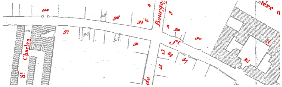
Figure 3. In this example, hand written text is automatically detected and extracted (red) from an historical map.
2.2. Modelling geohistorical objects
208
Information extracted from historical maps is used to create gazetteers. Those are made of
209
geohistorical objects. To this end, we design a geohistorical objects model with all necessary attributes
210
and also flexibility to adapt to the great variety of geohistorical object types and sources. Our goal is to
211
provide a generic minimal (geo)historical object model that can be used by other and easily extended
212
when necessary.
213
7 http://www.openstreetmap.org
2.2.1. modelling choices
214
Geohistorical data are extremely diverse, both in terms of historical sources and in terms of how
215
the sources were dealt with by historians. As such, historians use complex tailored models. We do not
216
aim at modelling all geohistorical data in all their complexity. Instead, we propose to model the bare
217
minimal common properties of all geohistorical objects, and offer mechanisms so this model can be
218
easily extended and tailored to the specificities of the data. To define the bare minimal model, we start
219
from the very nature of a geohistorical object, that is both an historical object and a geospatial object.
220
The extension mechanism is provided via a database-object oriented design using table inheritance,
221
and is packaged into a PostgresSQL extension9.
222
2.2.2. geohistorical objects model
223
Geohistorical objects have both an historical and a geospatial part. We stress that modelling
224
historical source and numerical origin process of a geohistorical object is an essential part. The detail
225
of the model are illustrated in Figure4.
226
Historical aspect
227
In our model, an historical object is defined by its name, source and temporalization.
228
• Name.By name, we mean the historical name that was used to identify the object in the historical
229
source, and the current name that is used by historians to identify the object in the current context.
230
For instance, the historical name of the Eiffel tower in Paris may be "tour de 300 mètres", but,
231
today, it is referenced as "tour Eiffel".
232
• Source.A historical object is defined by a primary historical source (document), where the object
233
is referenced. Beside the historical source, the way the object was digitized in this source is also
234
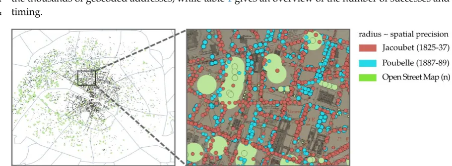
essential. For instance, a street name may have the Jacoubet topological map as historical source,
235
and would have been digitized via collaborative editing on the georeferenced map.
236
• Temporalization. Any historical source is associated with temporal information (fuzzy dates),
237
which is the period during which the source is likely relevant. Beside the historical source
238
temporal information, a historical object can also have its own temporal information. For
239
instance, a street may have been extracted from a historical map having been drawn between
240
1820 and 1842. Besides this information, using other historical documents allow to narrow the
241
probable existence of this street to 1824-1836.
242
Geospatial aspect
243
A geohistorical object is also defined by geospatial information: a direct spatial reference
244
(geometry) and its positional accuracy metadata.
245
• Geometry. A feature has a geometry which follows the OGC standard10. It may be a point,
246
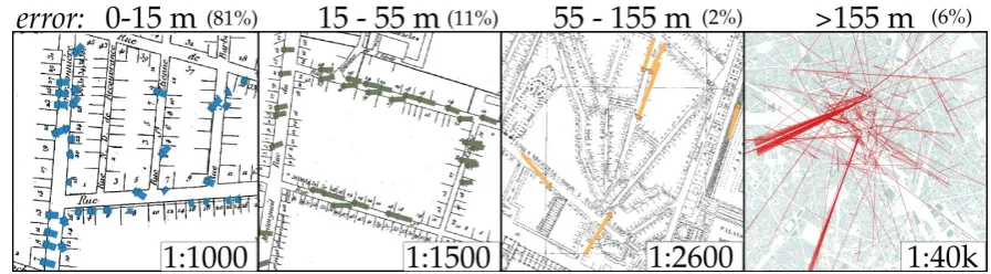
polyline, polygon, or a composition of any number of those, in a specified SRS. The geometry is
247
extracted from the historical source (in a manual or automatic way).
248
• Positional accuracy. Historical features have positional accuracy information. This precision
249
expresses the spatial uncertainty of the historical source (the person drawing the map may have
250
made mistakes) and the spatial imprecision of the digitizing process (the person editing the
251
digitised map may have made a mistake). One historical source may contain several accuracy
252
metadata, one for each geohistorical object type it contains. For instance, a historical map may
253
contain buildings and roads. Buildings may have a different positional accuracy (5 metres) than
254
road axis (20 metres). Besides, the digitising process precision may have been of 5 metres.
255
numerical_origin_process short_name
full_name description
default_fuzzy_date default_spatial_precision historical_source
short_name full_name description
default_fuzzy_date default_spatial_precision
geohistorical_object historical_name normalised_name geom
specific_fuzzy_date
specific_spatial_precision
historical_source
numerical_origin_process
Figure 4.The geohistorical object model, where each object is characterized by its historical source (for instance the historical map the object was described in) and a numerical origin process, which is the process through which the object was digitized. Besides source and origin process, an object is also described by a fuzzy date, a text and a geometry.
2.2.3. A database of geohistorical objects
256
We define a conceptual schema for geohistorical objects, which is based on two names, a source, a
257
capture process, fuzzy dates and a geometry. This defines the core of a generic geohistorical object.
258
Yet this geohistorical object model is easily extendible using the table inheritance mechanism, an
259
object-oriented design mechanism that is available in PostgreSQL (see Figure5).
260
Table inheritance
261
- historical_name - normalised_name - geometry
- specific_fuzzy_date - historical_source -numerical_origin_process
- historical_name - normalised_name - geometry
- specific_fuzzy_date - historical_source - numerical_origin_process - unique_id
- road_width ...
- historical_name - normalised_name - geometry
- specific_fuzzy_date - historical_source - numerical_origin_process - open_street_map_id - type_of_building - picture_id ...
parent table
child table 1
child table 2
Columns are inherited from parent
Still free to add other columns
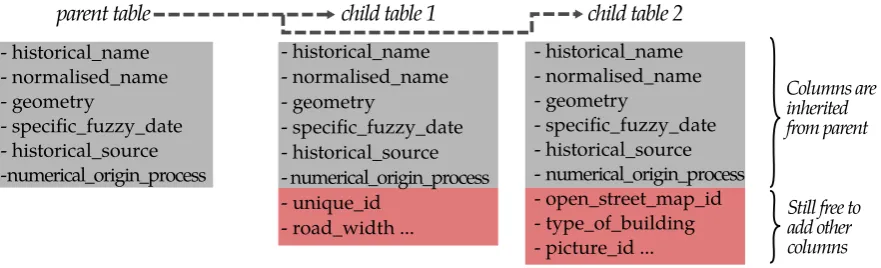
Figure 5.The table inheritance mechanism: a child table inheriting from a parent table inherits all the parent columns, and can also have its own.
The concept of table inheritance is simple. When a tablechildis created as inheriting from a table
262
parent,childwill have at least the columns ofparent, but can also have other columns (provided there
263
is no name/type collision). This means in our case that a table of geohistorical objects will inherit from
264
the main geohistorical object table,i.e.will have all the core columns of geohistorical objects (names,
265
sources, temporal aspect, spatial aspect), but can also have its own tailored column, providing the
266
necessary flexibility.
267
Another key aspect of table inheritance is that the parenttable is queried, the query will be
268
executed on not only the rows ofparenttable, but also on the rows of allchildtable. This means that
269
all tables using the geohistorical object model will be virtually grouped and accessible from one table.
270
Simulated inheritance of index and constraints
271
The PostgreSQL table inheritance mechanism is however limited in some aspects, because
272
constraints and index can not be inherited. Constraints are essential, because they are used to
273
guarantee that any geohistorical object will correctly use existing sources from the sources tables
274
("historical_source" and "numerical_origin_process"). Indexes are also essential, because when using
hundred of thousand of geohistorical obejcts, they are needed to help speed the queries. We index
276
not only names, but all geohistorical object core columns (names, sources, temporal aspect, spatial
277
aspect). We propose a registering function that the user can execute only once when creating a new
278
geohistorical object table.
279
Modelling a geohistorical object from the user perspective
280
The practical steps to create geohistorical objects are simple:
281
1. Add the historical source and numerical origin process in the source and process tables.
282
2. Create a new table inheriting geohistorical objects and containing your additional custom
283
columns
284
3. Use the registering function with this table name
285
4. Insert your data in the table.
286
2.3. Geocoding historical addresses with geohistorical object gazetteers
287
In the previous section, we explained how we create gazetteers of geohistorical objects from maps.
288
1. an historical map is scanned,
289
2. scans are georeferenced using hand picked control points,
290
3. historical work allow to estimate temporal information and spatial precision of the map,
291
4. roads name and axis geometry is extracted from the scan (manually or automatically),
292
5. building numbers are extracted from the scan (manually or automatically),
293
6. in some cases, building numbers can be generated from the available data,
294
7. normalised names are created from historical names,
295
8. geohistorical objects are created.
296
The next step is to use these gazetteers to geocode historical addresses.
297
2.3.1. Historical geocoding concept
298
In our method, geocoding something is finding the most similar geohistorical objects within the
299
available gazetteers, which then provides the geospatial information. This approach relies on two key
300
components: gazetteers of geohistorical objects, and a metric to find the best matches. This approach
301
allows to perform geocoding in a broad sense, as it does not rely on a structured address (number,
302
street, city, etc.), but rather on a non constrained name.
303
2.3.2. Creating geohistorical object gazetteers for geocoding
304
geohistorical object gazetteers are key for the geocoding. These objects are extracted from
305
topographical historical maps and inserted into geohistorical objects tables. Each table form a gazetteer.
306
Database architecture for geocoding
307
We again use the PostgreSQL table inheritance mechanism. To this end, we create two tables
308
dedicated to geocoding. Now gazetteers tables that will be used in geocoding must inherits from these
309
two tables. "precise_localisation" table is for building number geohistorical objects,e.g. "12 rue du
310
temple, Paris". "rough_localisation" table is for road axis, neighbourhood, cities geohistorical objects.
311
We chose to have two separate tables for ease of use and performance. Geocoding queries are then
312
performed on the two parents tables, but thanks to inheritance, these parents tables virtually contains
313
all the gazetteers table containing the actual geohistorical objects, as illustrated in Figure6.
314
2.3.3. Finding the best matches
315
Once geohistorical objects gazetteers describing precise and rough localisation are available,
316
geocoding is finding the best match between the input query and the objects.
precise_localisation geohistorical_object
associated_geohistorical_object
rough_localisation geohistorical_object geohistorical_object inherits
inherits extracted_building_numberprecise_localisation ...
inherits extracted_road_axisrough_localisation ...extracted_citiesrough_localisation
...
extracted_building_number precise_localisation ...
extracted_building_number precise_localisation ...
extracted_neighbourhoods rough_localisation ...
Geocoding queries
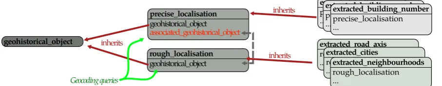
Figure 6.Geocoding table architecture. Two tables of geohistorical_object are the support for geocoding queries. Because all extracted geohistorical objects tables inherits from these two tables, they both virtually contains all the objects.
Concept
318
We call the potential matches "candidates", and the problem is then to rank the candidates from
319
best to worst. The user can chose how many candidates he wants, depending on the application. For
320
an automated batch geocoding, the best match (top candidate) is optimal. For a human analysis of
321
data, several matches may be more interesting (top 10 candidates for instance). What can be qualified
322
as "best" depends on the user expectations. We provide a number of metrics than can be combined by
323
a user into a tailored ranking function. The function is expressed in SQL, with access to all postgres
324
math functions. We describe the available metrics and give example of such function.
325
Example
326
For instance when a user geocodes the address "12 rue de la vannerie, paris" in 1854, user may be
327
more interested into geohistorical objects that are textually close (e.g.a geohistorical object "12 r. de la
328
vannerie Paris", 1810), or maybe geohistorial objects that are temporally close (e.g."12 r. de laTannerie
329
Paris",1860).
330
Metric: string distance wd 331
We use the string distance provided by the PostgreSQL Trigramm extension (pg_trgm11), which
332
compares two strings of characters by comparing how many successive sets of 3 characters are shared.
333
For instance "12 rue du temple" will be farther away from "12 rue de la paix" than from "10 r. du
334
temple".
335
Metric: temporal distance td 336
Both the address query and the geohistorical object are described by fuzzy dates. In order to
337
compare such temporal information, we propose a simple fuzzy date distance that casts fuzzy dates
338
into polygons. The x axis is the time, and the y axis is the probability of existence of the object. Then
339
the distance between twon datesAandBis computed as shortest_line_length(A,B) + Area(A) - Area(A
340
∩B). Note that this distance is asymmetric.
341
Metric: building number distance bd 342
To get building number distance, a function first extracts the building number both from the input
343
address query (bi) and from the geohistorical object (bd). Ifbiandbdhave same parity, the distance
344
is|bd−bi |. If parity is different, the distance is||bd−bi|+10|. In France, building numbers have
345
in general the same parity on each side of the street (e.g. Left : 1,3,5,.. ; Right: 2,4,6..). We analysed
346
current building number in Paris and determined that on average, given a building numberbi, the 347
closest building number with a different parity has a 10 number difference.
348
Metric: positional accuracy sp 349
Another way to rank the geohistorical objects is to use their positional accuracy. The positional
350
accuracy of a geohistorical object is either the positional accuracy computed for this objects when it is
351
available, or the default positional accuracy of its geohistorical source.
352
Metric: level of detail distance sd 353
Providing localisation information at different level of detail, depending on the user requirement
354
is an important quality issue for our geocoder. For instance if the level of detail of the user’s query data
355
is the city, there is no need to perform a more precise geocoding. Therefore the user can specify a target
356
scale range(Sl,Sh). Then given a geohistorical object whose geometry is buffered (geomb) with its
357
spatial precision, the scale distance is defined byleast(|p
area(geomb)−Sl |,|
p
area(geomb)−Sh|). 358
The formulap
area(geomb)gives an idea of the spatial scale of the geohistorical object.
359
Metric: geospatial distance gd 360
The user may provide an approximate position for the area he is interested in. For instance in
361
France both city "Vitry-le-François" (East) and "Vitry-sur-Seine" (near Paris) exist, but are very spatially
362
far away. A user expecting results in the Paris area may provide a geometry (a point for instance)
363
near Paris. Then the classical geodesic distance is computed between the provided geometry and the
364
candidates geohistorical object.
365
Example of matching function
366
The different metrics can be weighted and combined depending on the user needs. Equation1
gives an example that favour good string similarity, but not at the price of a large temporal distance.
100∗wd+0.1∗td+10∗nd+0.1∗sp+0.01∗sd+0.001∗gd (1)
2.4. Collaborative editing of geohistorical objects
367
The geocoding approach we have presented in the previous section works inside a PostgreSQL
368
database. Given an input address and fuzzy date, plus a set of parameters, it returns the geohistorical
369
objects that matches the input the best. Yet the geocoding results are only as good as the gazetteers
370
used. The geohistorical objects within the gazetteers may be spatially imprecise, mistakenly named
371
or simply missing. Given that the volume of geohistorical objects is large (for Paris, approximately
372
50 k building number per historical map), we create a collaborative platform to facilitate geocoding,
373
visualising the results and editing the geospatial objects when necessary. To this end, we create a
374
dedicated web application so collaborative editing is possible without having to install specific tools.
375
2.4.1. About collaborative editing
376
Given the complexity of calibrating automatic extraction tools on specific maps and their relative
377
reliability, the collaborative digitisation of vector objects from maps is a safe alternative. For instance,
378
we used such an approach in order to extract the main feature of the Cassini maps (18th century
379
France) [25]. Furthermore, the results of the collaborative extraction of features can then be used to
380
test, calibrate or train automatic extraction algorithms.
381
2.4.2. Collaborative editing architecture
382
Figure7outlines the architecture used for collaborative editing.
Figure 7. Conceptual architecture for interactive display and edit of geocoding results. The stack ocntains only standard components.
Architecture
384
The hearth of the architecture is a PostgreSQL database server, which contains the geohistorical
385
objects gazetteers that will be used for geocoding as well as the geocoding function. A webserver can
386
geocode addresses and return results via a REST API. However, the webserver has another option
387
where the results are not returned, but instead written in a result table along with a random unique
388
identifier (RUID). The RUID is then the key that permit to display and edit the results. To this end, a
389
geoserver can access (read and edit) the result table via the WFS-T protocol. A web application based
390
on Leaflet then acts as a user interface to display and edit the results via the geoserver.
391
Persistence of geocoding results and edits
392
Postgres Geoserver
Leaflet Rest API
/interactive_session
- Create unique session_id - Fill result table with (results,session_id) - returns session_id (adress, date,etc)
result
gid geom ... session_id
1 Point(..) Xue87..12 5 Point(..) aiElez..65
result_view
gid geom ... session_id
1 Point(..) Xue 5 Point(..) aiE
classic view, except show only beginning of session_id
read
trigger : edit only if matches on (gid, session_id) using full session_id - ask for interactive
geocoding with (adresse,date,etc.) - receive unique session_id "aiElez..65"
WFST - show results of geocoding having session_id starting with "aiE"
GEOCODE
VIEW RESULTS
WFST - edit point: send (new_geom,...,session_id) (POINT(..),...,"aiElez..65")
EDIT RESULTS
SERVER CLIENT
layer result_view USER
write
Figure 8.Collaborative display and edit is achieved through a mix of standards (REST , WFS-T) and custom solution (triggers) that enable the sharing of a basic public/private key.
The architecture that allows persistence of results is illustrated in Figure8. When using the
393
RUID mechanism, each geocoding result (that is the found geohistorical object from the gazetteers) is
394
associated to this RUID. That way the user can always access its results, regardless of the computer
395
session or browser cache issues.
396
To edit, a specific mechanism is used. The user does not directly edit the result table, as he could
397
potentially edit other people results. Instead, the user edit a dedicated result_view that acts like a
398
bouncer. It allow edit only if the edit is occurring on a row that has the user RUID. User edit of the
399
geospatial objects do of course not affect the source data, for a tracking purpose.
400
Instead, a new user edit automatically creates an edited copy of the geohistorical object in a
401
dedicated table "user_edit_added_to_geocoding" that is a gazetteer and is used by the geocoding
process. In this table are inserted the edited geohistorical objects. The objects retain their
403
"historical_source", but their "numerical_origin_process" is changed to properly document the fact that
404
they are the result of a collaborative editing.
405
2.4.3. Collaborative editing user interface
406
We consider that building an efficient user interface is very important for historical geocoding. In
407
particular, many end users are specialised on history rather than on computer science, and thus an
408
easy access to geocoding is essential. All our interfaces are web-based for a maximum of compativility.
409
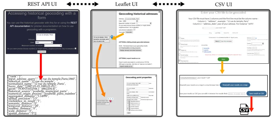
We propose three interfaces whose results are shared.
410
[{"rank":"1",
"input_adresse_query":" 12 rue du temple,Paris;1860", "historical_name":"12 rue du temple",
"normalised_name":"12 rue du temple ,Paris", "fuzzy_date":"[1887-01-01,1889-01-01)", "geom":"POINT(652544.1 6862204.4)", "historical_source":"poubelle_municipal_paris" , "numerical_origin_process":"poubelle_paris_number", "aggregated_distance":"3.14999",
"spatial_precision":"3.5", "confidence_in_result":"1", "semantic_distance":"0", "temporal_distance":"28", "number_distance":"0", "scale_distance":"0", "spatial_distance":"0"}]
REST API UI Leaflet UI CSV UI
Figure 9.Various Web User Interface for use of historical geocoding.
Interface for a REST API.
411
The simplest interface we propose is a form that helps build the necessary REST API parameters.
412
Indeed, a REST API works via URL containing precise parameters, and it can be tedious to manipulate.
413
For instance:
414
https://www.geohistoricaldata.org/geocoding/geocoding.php?adresse=2012ruedutemple,Paris&
415
date=1860&number_of_results=1&use_precise_localisation=1
416
This interface is designed to be used in an automated way, for batch geocoding.
417
Interface for batch geocoding via CSV files.
418
In our experience historian often work with spreadsheet files, where each line will be a potential
419
historical object, along with an address and a date. To facilitate the geocoding of these addresses,
420
we propose a User Interface that can read Coma Separated Value (CSV) files (which is a standard
421
spreadsheet format), and geocode the address and date within. This interface is built around
422
PapaParse12 Javascript framework. Then, the geocoding results can be either downloaded as a
423
CSV file, or displayed and edited in a web application.
424
Interface for display and edit of results.
425
The most complex interface we propose is based on the Leaflet13Javascript framework. There, the
426
user can geocode an address, or use already geocoded address via the RUID mechanism (see Section
427
2.4.2.1), be it from previous sessions or from geocoded CSV files. The geocoding results are displayed
428
on top of a relevant historical map, and can be edited. User can edit results geometry as well as results
429
names (historical and normalised). We stress that although such edit are stored in the database, and
430
used by further geocoding queries, they do not affect source data, by design.
431
3. Results
432
We perform several experiments to validate our approach. First we use the geohistorical model to
433
integrate objects extracted from historical topographical maps from the 19th century for the city of
434
Paris, and the current OpenStreetMap road axis and building numbers for Paris city surroundings.
435
We successfully integrate the road axis, building numbers, and neighbourhoods to the geocoder
436
sources. We then perform multiscale geocoding of dozens of thousand of historical addresses extracted
437
manually by historians and extracted automatically by automatic process. For one of our datasets, we
438
ask the historian to manually correct the automated geocoding results, so as to evaluate the quality of
439
our method. Last, we test the collaborative editing of geohistorical object in two scenarios: analysis
440
(several results for one address), and edit (efficiency of check/edit top results for several addresses).
441
3.1. geohistorical objects sources
442
We mainly use three historical sources of geohistorical objects to perform geocoding. The first two
443
are Historical topographic maps of Paris from the 19th century. These maps are georeferenced then
444
street axis (and possibly building numbers) are manually extracted. The third historical sources are
445
road axis and building number for Paris surrounding extracted from current Open Street Map data.
Figure 10.geohistorical objects used from geocoding extracted from the source maps.
446
3.1.1. Historical topographic maps used
447
We integrated two major French atlases of Paris from the 19thcentury as geohistorical sources.
448
The first one is the "Atlas municipal de la Ville, des faubourgs et des monuments de Paris"14created
449
at the scale of 1 : 2000 between 1827 and 1836 by Theodore Simon Jacoubet, an architect who was
450
working for the municipal administration of Paris. The second atlas is the 1888 edition of the "Atlas
451
municipal des vingts arrondissements de la ville de Paris"15. For legibility reasons, we refer to the first
452
13 http://leafletjs.com
atlas as the "Jacoubet atlas" and the second as the "Alphand atlas"16. The Jacoubet atlas depicts a city
453
standing between the housing development following the sale of the properties confiscated during the
454
French Revolution and the majors changes in the urban structure arising from the emergence of the fist
455
train stations in 1837-1840 and the so-called Haussmannian transformations.
456
The Alphand atlas is a portray of Paris at the scale of 1 : 5000, after most of the Haussmannian
457
transformations (major rework of Paris urbanism in the 19th century) and after the city was merged
458
with 11 of its neighboring municipalities in 1860. Both atlases contain large scale topographic views of
459
Paris, separated in several sheets (54 and 16 respectively) and portray the urban street network with
460
each street named, building of public purposes and religious buildings (see Figure11). In addition, the
461
house numbers are specified for most of the streets in the city, although the Alphand atlas pictures only
462
the numbers at the start and end of each street section. Both atlases are also built upon triangulation
463
canvas covering the entire city, allowing us to expect a high positional accuracy of the geographical
464
features they contain.
465
Figure 11. Samples of the georeferenced Alphand Atlas (2ndrow) and Jacoubet Atlas (1rstrow) at different scales: district (a) and urban islet (b). Column (c) shows how buildings are portrayed in the maps.
We georeferenced the two atlases using the grids drawn on the maps, which are aligned on the
466
Paris meridian, as a pseudo-geodetic objects to identify feature pairs. The dimensions of the grid cells
467
also appear on the maps, allowing us to reconstruct the grids in a geographic reference system. We
468
have chosen to georeference the maps in the Lambert I conformal conic projection, which uses the
469
Paris meridian as prime meridian and rely on the NTF (Nouvelle Triangulation Française) geodetic
470
datum. The main advantage of this projection is that it is locally close to the planar triangulation of
471
Paris used in the atlases. Thus, the projection of the maps can be reasonably approximated by the
472
Lambert I projection, making the reconstruction of the grids in the target coordinate reference system
473
straightforward. In addition, since both maps are at high scale and are reliable because they are official
474
maps with high positional accuracy, we used rubbersheeting as the geometric transform model. The
475
georeferencing process applied for each atlas was the following:
476
• reconstruct the meridian-aligned grid with Lambert I coordinates;
477
• in each sheet, mask the non-cartographic parts out (cartouche, borders,etc.);
478
• for each sheet, set pairs of ground control points at each intersection between the vertical and
479
horizontal lines of the grids in the map and in the reconstructed grid;
480
• transform each sheet with a rubbersheeting transform based on the ground controls points
481
previously indentified on the grids.
482
geohistorical objects extraction
483
Based on these atlases, vectorial road axis are manually drawn and the road name inputed For
484
Alphand map, the building number at the beginning and end of ech street segment is also inputted.
485
For Jacoubet, the building numbers from a previous map (Project Alpage, Vasserot map, [26]) are
486
adapted to fit the Alphand map. Multiple series of successive checking and editing are performed
487
using ad hoc visualisations and tools.
488
For Alphand, building numbers are then generated based on the available information (for each
489
street segment, for each side, beginning and ending number) by linear interpolation, and an offset.
490
The size of the offset is estimated by using current Paris road width when the road has not changed to
491
much.
492
3.1.2. Other geohistorical sources
493
We also use current data from OpenStreetMap. We use the version of the data that has been
494
transformed to be used by the Nominatim geocoder. Custom scripts extract road axis and building
495
numbers. The dataset covers Paris city and its surroundings, and is dated to 2016.
496
3.2. Geocoding of Historical datasets
497
One of the end goal of our geocoding tool is to be useful for historians. Therefore, we contacted
498
several historians working on Paris (19th century). They had been collecting historical addresses,
499
which we geocoded by importing their data into the geocoding server. Figure12shows an extract of
500
the thousands of geocoded addresses, while table1gives an overview of the number of successes and
501
timing.
502
Figure 12.All geocoded historical datasets. Size is proportional to spatial precision.
3.2.1. Manually collected dataset
503
South Americans:South America immigrants living in Paris in 1926, manually input from census,
504
collected by Elena Monges (EHESS).
505
Textile:Professionals of textile industry in Paris, manually input from the "Almanachs dy Commerce
506
de Paris", from 1793 to 1845, collected by Carole Aubé (EHESS).
507
Artists accommodations:Addresses of artist studios and artists accommodations between 1791 and
Table 1.All geocoded historical datasets facts.
Dataset name input addresses response rate (rough) secs/1000 addresses
South Americans 13991 13743 (250) 138
Textile 5777 5688 (16) 135
Textile 2 3070 3053 (2) 110
Artists accommodations 13907 10215 (2955) 244
Health administrators 1887 1698 (171) 316
Belle epoque (0.3) 6467 3880(337) 280
Belle epoque (0.5) 6467 6000 351
1831, collected by Isabelle Hostein (EHESS) to study their impact on Paris development.
509
Health administrators:Addresses of public health and hygiene administrators in Paris between 1807
510
and 1919 ([27]), collected by Maurizio Gribaudi and Jacques Magaud (INED-EHESS).
511
3.2.2. Belle epoque
512
We geocode another set of addresses that are automatically extracted from directory of Paris
513
financial societies between 1871 and 1910. Directories are books referencing address of company (and
514
name and other information). The process of automatic extraction is complex in itself (Project Belle
515
Epoque, [28]), and is out of scope of this article. We only describe it briefly here.
516
First, each page of the directories of Paris for specific years are photographed. Pictures are then
517
straightened, and information is extracted via an OCR software which has been configured for the
518
directory specific layout. Further rule based processing parse the text into address fields. As a result
519
of this automatic process, the quality of addresses is often significantly lower than manually edited
520
addresses. Therefore, we test two settings by allowing a greater maximum string distance from 0.3 to
521
0.5 (over 1).
522
3.3. Manual editing of the geocoding results for evaluation
523
Figure 13.An historian manually move the geocoded addresses.
For one of the data set (Textile 1 and 2), the historian manually correct the geocoded results. We
524
then plot the segment between address point resulting of automated geocoding and address point
525
after manual editing. Results are presented in the table2and in Figure13We classify the results based
526
on the length of this segment (i.e.the error in meter the geocoding method made).
527
• When the edit move the adress point less than 15 meters, we can consider that the edit is mostly
528
about small moves , for instance centering the point on the building limit.
529
• Between 15 and 55 meters, the correct street has been found, but the building numbers are slightly
530
misplaced (a few numbers).
531
• Between 55 and 155 meters, in most cases the street is correct, but the building numbers are far
532
from their correct position.
Table 2. Evaluating the error of geocoded results, via the dist. (geographic distance) of edit, the percentage of the total 8823 addresses, the average aggregated distance score, the average string distancewd, the average temporal distance td, and the subjective most common edit reason we encountered while browsing the data
dist. (m) % avg(agg) avg(sem) avg(tempo) main edit cause (subjective)
0 - 15 81 % 9.4 0.07 19.5 moving point on building limit
15- 55 11 % 12.4 0.09 27.2 small numbering editing (same street) 55 - 155 2 % 23.7 0.14 41.2 large numbering editing (same street)
155 - 7.2k 6 % 26.9 0.18 49.1 editing street
• Above 155 meters, streets are wrong in most of the case.
534
We stress that given Paris building average size, and the lack of precise definition of an address (is
535
it the position of the door, of the center of the building,...?) results up to 55 meters could be considered
536
as very close to ground truth.
537
3.4. Collaborative editing
538
We propose several User Interface for easy geocoding, and collaborative editing of the geocoding
539
results. We informally tested the interfaces and found that they facilitate geocoding, especially for the
540
batch mode. We also test the collaborative editing in two use cases. In the first use case a specialised
541
user geocodes a single address and display the top 3 results corresponding to this address. The user is
542
expert and its goal is geocode an address and assess the reliability of the result at the same time. In the
543
second use case, a user batch geocode several addresses (30), looking of the best result for each adress.
544
Then the user display the results on the map and check/edit the adresses.
Figure 14.Two use cases: First use case, an expert geocodes an address and analyse the top 3 results to assess the reliability of the result. Second use case: a user batch geocodes 30 addresses ( 1 result per address) in Paris and chek/edit the results.
545
3.4.1. Use case 1: top 3 results for one address
546
Using the web application, we geocode the address "10 rue de vaugirard, paris" for the date 1840,
547
and ask for the top 3 results, as shown in first part of illustration14. A matching building number
548
geohistorical object exists in the three gazetteers extracted from the three maps. Based on the results,
549
we can safely assume that this building number has not changed during the last 2 centuries.
550
3.4.2. Use case 2: batch geocoding of 30 addresses and check/edit
551
In this use case, a regular user is to check/correct 30 random addresses from the Jacoubet map
552
using the web application. The task is performed quickly, the check and edit of each address is a matter
553
of a few seconds. The main time consuming task is the loading of the background historical map, due
554
to unfortunate hardware limitations. The edit speed seems to be on par with a desktop based edit
555
solution (using QGIS).
4. Discussion
557
4.1. Genericity
558
Reaching a more generic geocoding service is important if we want to make it usable in other
559
contexts and to profit from the various sources of knowledge on past spaces.
560
4.1.1. Geohistorical sources and data
561
Using external resources from the Web of data as new sources
562
Besides features representing address points and streets, georeferenced features of other types
563
could be used with benefits by the geocoding service. As a matter of fact, people often refer to
564
places of interest, such as famous buildings, monuments like statues or fountains or even named
565
neighbourhoods to describe their position in space. We thus consider adding data about places of
566
interest to improve our geocoding service. Like the data that was used to build the geocoder, such data
567
could be gathered from ancient maps. But they may also come from existing gazetteers and knowledge
568
bases published on the Web of data, such as DBpedia17, Yago18, the Getty Thesaurus of Geographical
569
Names19or the gazetteer of place names published by the French National Library20.
570
Widen the spectrum of cartographic sources
571
We exploit Jacoubet and Alphand maps, yet there are several more to be exploited toward the end
572
of the 19th century, and in the beginning of the 20th century. From the beginning of the 20th century,
573
Paris city administration produced a map per year. Of course, the main improvement direction would
574
be to add maps of other cities/countries! For France at least, major cities have often been mapped
575
starting from 1900.
576
Before the beginning of 19th century, the address system was very different in Paris. in mid 18th
577
century, the address system was in fact that each building would have a specific name (no number, no
578
notion of street name) in its neighbourhood. Our geocoding system has also been designed with this
579
type of addressing but it has not been tested yet. More generally, this type of indirect localisation is
580
very close to the field of web of knowledge.
581
Diversity in geohistorical objects natures
582
In this article several type of geohistorical objects were used for geocoding: building numbers,
583
streets axis, neighbourhood. Other datasets were investigated as well, such as the city limits extracted
584
by the project Geo Historical Data in a collaborative way from the Cassini maps [25]. In fact, a compiled
585
version of city limits (GeoPeuple project [29]) from 1793 to 2010, created by EHESS, has also been
586
tested. But building cadastres could also be integrated so as to have a building layout associated to
587
an address rather than a point, which would solve an old problem of address points. Indeed, there
588
is currently no consensus as to where a building number address point should be positioned: on the
589
entry door, on the letter box, etc. More excitingly, in some cases, more precise data is available, giving
590
the layout of apartments in buildings.
591
17 http://wiki.dbpedia.org/
18 http://www.mpi-inf.mpg.de/departments/databases-and-information-systems/research/yago-naga/yago/#c10444
4.1.2. Genericity in usages
592
Named Entity Linking
593
As we mentionned in section4.1, people often refer to place names to describe their position in
594
space. The task of retrieving place names in a gazetteer or in a knowledge base, also known as (Spatial)
595
Named Entity Linking or toponym resolution, is a widely used way of desambiguating mentions
596
of spatial named entities extracted from texts by means of natural language processing approaches
597
for information retrieval, information extraction or document indexing purposes [30]. As we plan
598
to upgrade our geohistorical database with data about places of interest, we also have to adapt our
599
geocoding service in order to make it retrieve reference data stored in the database and corresponding
600
to place names mentions proposed by the users. Spatial Named Entity Linking implies solving issues
601
related to places names inherent ambiguity [31], such as the fact that a place may have several names
602
or the fact that several places may be designated by the same name. For each spatial named entity
603
mention to be disambiguated, unsupervised state of the art approaches first select candidates from
604
the gazetteer based on character string similarity. Then, they introduce additional criteria in order to
605
decide which candidate is the best reference for a given place name, usually taken from the textual
606
context of the mention [32,33]. In cases where textual context is very limited, like in tweets or location
607
descriptions extracted from directories, this step of candidate ranking reveals even more challenging
608
[34].
609
Analysis tool of the cartographic sources content
610
It is interesting to look at what historical sources were the most used for geocoding, although
611
the historical source are chosen based on a complex ranking function. If we take the example of the
612
over 10k geocoded addresses from the "Artists accommodations" dataset, we could expect all of the
613
results to be drawn from the Jacoubet map, as the dataset is between 1793 and 1836, and the Jacoubet
614
map is also in this range. Yet, analysing the results shows that if Jacoubet was used for 80% of the
615
addresses, Alphand was used for 15%, although the map comes 30 years after. More surprisingly, the
616
OpenStreetMap current data is still used for 5% of addresses, although it is about 2 centuries after the
617
dataset.
618
Similar analysis on other datasets show similarly that all maps are always used, with of course a
619
focus on the temporally closest map. Interestingly, these results are in agreement with similar work as
620
presented in [35], chapter 4, where a prototype of multi-temporal geocoding is proposed. The approach
621
shows that for different datasets, all references maps (Jacoubet, Alphand and BDAdresse (2010)) are
622
used, with proportions depending on the parameters considered and the weights of each criteria. We
623
think that this results are explained by the fact that historical maps miss some information, contain
624
errors, and do not have the same geographical coverage.
625
4.2. Quality of the geocoding
626
4.2.1. Increasing the quality of the gazetteers
627
Collaborative enrichment
628
We propose several ways to use the geocoding capabilities in an easy way through web based
629
User Interfaces. As we propose prototypes, the experiments are merely proofs of concepts for the
630
moment. For a real validation, a complete user study would be required, which is outside of the scope
631
of this article.