Mesh Optimization for Maxwell’s Equations with Respect to
Anisotropic Materials Using Geometric Algebra
Mariusz Klimek1, *, Sebastian Sch¨ops1, 2, and Thomas Weiland2
Abstract—Clifford’s Geometric Algebra provides an elegant formulation of Maxwell’s equations in the space-time setting. Its clear geometric interpretation is used to derive a goal function, whose minimization results in Hodge-optimized material matrices being diagonal or diagonal-dominant. Effectively it is an optimization of the primal/dual mesh pair of a finite difference based discretization scheme taking into account the material properties. As a research example, a standing wave in 2D cavity filled with an anisotropic material is investigated. Convergence of the scheme for various choices of mesh pairs is discussed. The limitations of the method in the 3D case are presented.
1. INTRODUCTION
Clifford’s Geometric Algebra (GA) in the context of discretization of Maxwell’s equations is closely related to the Cell Method [3], Discrete Exterior Calculus [10] and to the Finite Integration Technique (FIT) [4]. All schemes are based on finite differences. For example, FIT allocates the electromagnetic quantities on points, edges, facets and three dimensional volumes of a primary and a dual grid such that they are natural discretization in terms of exterior algebra and differential forms. The time domain is typically treated afterward by the leap-frog scheme. On the other hand, the GA-based approach differs from that as it naturally performs discretization in space-time, i.e., taking immediately into account all four dimensions. Compared to the exterior algebra of differential forms GA gives more algebraic tools at the cost of explicit introduction of the metric. However, all approaches lead to practically equivalent schemes. This has been shown for the Cartesian grid case in [2].
The material relations link the quantities located at both, the primal and dual grid. In this paper we aim for grid conditions that allow to represent the relations as one-to-one connection of those quantities, i.e., one primal degree of freedom is linked to exactly a one dual. This is equivalent to diagonalizing the discrete Hodge star operator and yields eventually diagonal material matrices. The importance of this property comes from its impact on efficiency of the scheme: many matrix-vector multiplications and inversions of material matrices are carried out in the leap-frog time-integration of FIT-like schemes. This is obviously computationally more efficient and requires less data-storage if the matrices are diagonal. Attempts to achieve one-to-one properties via optimization of primal/dual mesh pairs in different context have been proposed, for example in [7]. However, in our case the Hodge star depends on material distributions which may be inhomogeneous, making it a function of space. Several formalisms have been proposed in related settings, for example anisotropic materials have been theoretically studied in [8] using classical tensor calculus, while differential forms have been used to recast Maxwell’s equations in [9]. However, here GA was chosen due to its clearer geometric interpretation
Received 4 November 2015, Accepted 4 February 2016, Scheduled 1 March 2016
* Corresponding author: Mariusz Klimek ([email protected]).
compared to other formalisms. Nonetheless a translation of the results in terms of differential forms is straight forward.
The paper is structured as follows. In Section 2, GA is briefly outlined. The focus is on space-time algebra. For illustration, we present how complex numbers can be derived as a subalgebra in the 2D plane showing that GA may be perceived as a generalization of complex numbers to higher dimensional spaces. Section 3 is devoted to recasting Maxwell’s equations in space time using space-time algebra. The integral form is preferred as it simplifies the derivation of the discretization. In Section 4, we discretize Maxwell’s equations with special attention on material relations. The main result is a sufficient condition that guarantees diagonal material matrices. Section 5 is an application of the theory to the simple 2D problem. Comparison with existing approaches is performed. Section 6 shows the limitations of the method in 3D. In Section 7 the conclusions are drawn.
2. GEOMETRIC ALGEBRA OF MINKOWSKI SPACE-TIME
In GA, the fundamental operation is thegeometric product of vectors, which is [1]
ab=ba, (noncommutative)
(ab)c=a(bc), (associative)
a(b+c) =ab+ac, (left-distributive) (a+b)c=ac+bc, (right-distributive)
a−1 = a
a2, (invertible)
wherea,b and care vectors. A norm is defined through |a|2 :=a2 ∈R. The geometric product of two vectors can be split into its symmetric (scalar) and antisymmetric (bivector) part
ab= 1
2(ab+ba) + 1
2(ab−ba) :=a·b+a∧b, (1)
where · and ∧ denote the scalar and exterior product. 4D Euclidean basis vectors are denoted by
γi,i∈ {x, y, z, t}, where x,y, z are space coordinates, and t is time. The convention is γt2 = +1 and
γx2 =γy2=γz2 =−1. Note that a vector is usually interpreted as an oriented 1D object. Thepseudoscalar
I :=γtγxγyγz gives a unique representation of any oriented 4D object (“space-time volume”)A4through
A4 = |A4|I. Its square is I2 = −1. Relative 3D vectors σk := γkγt, k = x, y, z, square to +1 and
are mutually orthogonal. Therefore, they are basis vectors of 3D space, but still (implicitly) contain temporal information. Additionally,I =σxσyσz holds. We denote relative 3D vectors by, e.g.,
E ≡Exσx+Eyσy+Ezσz. (2) The geometric derivative can be expressed as
∇=γα∂α=γt∂t+γx∂x+γy∂y+γz∂z =γt∂t−γx∂x−γy∂y−γz∂z, (3) whereγαare reciprocal basis vectors, i.e.,γα·γβ =δβαwhereδβαdenotes the Kronecker delta. Therefore, ∇ is a vector from the algebraic perspective and an operator acting on the object on its right from operational point of view. The relative 3D geometric derivative takes a similar form
∇=σi∂i =σx∂x+σy∂y+σz∂z. (4)
For the comprehensive introduction of geometric calculus the reader is referred to [5].
2.1. Complex Numbers
For motivation, we show that complex numbers are a subalgebra of 2D GA. Suppose we are given a vector r in the 2D plane. We define the real axis asx-coordinate line. The induced unit basis vectors areex and ey. Please note that we can define the real axis as any line in the plane, i.e., we can choose arbitrary unit vector instead ofex. Then we identify the complex numberz associated withr with
First, we note that the 2D pseudoscalar I := exey commutes with every complex number. Therefore, the algebra of complex numbers is commutative. Secondly, we see that its square is
I2 =II =exeyexey =−exexeyey =−1. (6)
Therefore, it is natural to identify I with the imaginary unit. The complex conjugate ofz isz†=rex. Suppose we are given a complex functionf =u(x, y)+Iv(x, y). Then we can state the Cauchy-Riemann equations as∇f = 0. We show it by expanding
∇f = (ex∂x+ey∂y) (u+Iv) =ex(∂xu−∂yv) +ey(∂yu+∂xv) = 0 (7) and noting that the equations in brackets are exactly the Cauchy-Riemann equations. Therefore,∇f = 0 holds for all analytic functionsf. The result is less surprising if we multiply this condition byex from the left and note that
ex∇=ex(ex∂x+ey∂y) =∂x+I∂y = ∂
∂x−
1
I ∂ ∂y =
∂ ∂(x−Iy) =
∂
∂z† (8)
Therefore, Eq. (7) is equivalent to more familiar property of analytic functions ∂z∂f† = 0, where inf we changed the coordinates from (x, y) to z =x+Iy and z† =x−Iy. Operations on complex numbers have a clear geometric interpretation in the 2D plane and this remains a characteristic feature of GA in arbitrary dimensions.
3. MAXWELL’S EQUATIONS
The traditional form of Maxwell’s equations separating space and time reads
∇ ×E =−∂tB
∇·B = 0
∇ ×H =∂tD +J
∇·D =ρ, (9)
whereρ,J,E,H,D andB are the electric charge density, electric current density, electric and magnetic field strengths, electric and magnetic field fluxes, respectively. Since Maxwell’s equations are Lorentz invariant, we express them explicitly in space-time [1]
∇ ∧F = 0 ∇ ·G=J, (10)
where F := E +I B, G := D +I H and J := (ρ+J)γ0. γ0 is the four-velocity of the medium. If
the medium is at rest, thenγ0 =γt. To derive the space-time form of Maxwell’s integral equations we
follow Hestenes [6]. We integrate (10) over an arbitrary bounded 3D star domain Ω⊂ Ξ, Ξ being 4D space-time, and apply the fundamental theorem of geometric calculus [5, 6]. The obtained equations are coordinate-free, do not involve any differentiation and are ready to be applied to an arbitrary 3D space-time element:
∂Ω
d2x·F = 0 and
∂Ω
d2x∧G=
Ω
(d3x)∧J. (11)
Both Equations (11) are linked by material equations given by
D=D
E, B
and H =H
E, B
. (12)
Ohm’s law is disregarded in this article. Thematerial mapping ξ is implicitly defined by
G=D
E, B
+IH
E, B
=ξ(F), (13)
where E = 12(F −γ0F γ0) and B = 21I(F +γ0F γ0). We want to stress that the introduction of ξ is
not a complication of the material equations but a translation to the space-time algebra in a consistent manner.
For example, if the medium is isotropic, i.e., permittivity εand reluctance ν are scalars in
we can directly calculate Gin terms of F in the coordinate frame of the medium
G=D +I H=ε E+νI B =ε1
2(F −γ0F γ0) +ν 1
2(F +γ0F γ0) = 1
2[(ε+ν)F−(ε−ν)γ0F γ0], (15) therefore we obtain a simple coordinate-free form of ξ for isotropic media
ξ(X) = 1
2[(ε+ν)X−(ε−ν)γ0Xγ0]. (16)
However, in this paper we are interested in more complex case of symmetric anisotropic media, i.e.,
DE, B= (σx, σy, σz) εεxxxy εεxyyy εεxzyz εxz εyz εzz
Ex
Ey Ez
(17)
and
HE, B= (σx, σy, σz) ννxxxy ννxyyy ννxzyz νxz νyz νzz
Bx
By Bz
. (18)
In this case using the explicit definition ofξ obtained by inserting (17) and (18) into (13) one can verify that
ξ(B1)·B2 =B1·ξ(B2) (19)
holds for all bivectors B1 and B2. Therefore, the material mapping is self-conjugate. Instead of
presenting a general expression for ξ we rather present a few important special cases. Sinceξ is linear, to evaluate for arbitrary F
ξ(F) =ξ(E) +ξ(I B) =Eiξ(σi) +Biξ(Iσi) (20) it is sufficient to know
ξ(σi) =εijσj and ξ(Iσi) =νijIσj. (21)
For the inverse ξ−1 the interesting equations are
ξ−1(σi) =ε−1ijσj and ξ−1(Iσi) =μijIσj, (22)
where permeabilityμ=ν−1.
4. DISCRETE SETTING
We discretize the 4D spacetime domain Ξ into a set of primal cells Ξi. The boundary of each primal cell consists of 3D volumes Ωk and the boundary of each Ωk consists of 2D facets Δj. We define edges and points in a similar manner. The structure above is referred as the primal mesh. A second, dual mesh is introduced in a similar fashion. Dual cells, dual volumes and dual facets are denoted byΞi,Ωk and Δj, respectively. The meshes are constructed in such a way that each Ξi contains exactly one dual node, each Ωk intersects one dual edge, each Δj intersects oneΔj, etc.
A discrete version of Maxwell’s equations “Maxwell’s 4D grid equations” is obtained by applying the left equation of Eq. (11) to each primal volume, and the right one on Eq. (11) to each dual volume:
∂Ωk
d2x·F = 0 and
∂Ωk
d2x∧G=
Ωk
d3x∧J. (23)
These integrals are sums of integrals of the type
fj :=
Δj
d2x·F and gj :=I−1
Δj
which we define as scalar degrees of freedom (DoF) on the primal and dual mesh respectively. The approximate fieldsFj∗ described by degrees of freedom follows from
fj =
Δj
d2x·F ≈
⎡ ⎢ ⎣ Δj
d2x
⎤ ⎥
⎦·Fj =Wj·Fj =WjFj∗, (25)
whereFj is the fieldF(xj) at some pointxj ∈Δj (typically the center),Wj is the bivector representing the magnitude and the mean orientation of the facet Δj
Wj :=
Δj
d2x (26)
and Fj∗ is defined such that the last equality in Eq. (25) holds
Fj∗ :=Wj−1(Wj ·Fj), (27) i.e., it is the projection ofFj onto the primal facet. The approximate field Fj is thus decomposed into the part Fj∗ stored in the degree of freedomfj and the partF0
j not stored at Δj
Fj =Fj∗+Fj0. (28) Performing similar manipulations on the dual mesh we are lead to
Igj ≈WjG∗j (29)
and the analogous decomposition into stored and not-stored fields
Gj =G∗j +G0j, (30) where
Wj :=
Δj
d2x, G∗j :=Wj−1
Wj∧Gj
and Gj :=G(xj), xj ∈Δj. (31)
To illustrate the steps made above, we consider a special case when Δj is a rectangle in (t, z) plane: Δj = [t1, t2]×[z1, z2]. We note that the DoF
fj =
Δj
d2x·F =
t2 t1 dt z2 z1
dzγzγt·F =
t2 t1 dt z2 z1
dzEz (32)
is related only to the z component of the electric field Ez. The bivector representing the rectangle is simply calculated
Wj =
Δj
d2x=
t2 t1 dt z2 z1
γzγt= ΔzΔtγzγt= ΔzΔtσz. (33)
The approximate fieldFj =E(xj) +I B(xj), wherexj ∈Δj. The stored component of the approximate field is
Fj∗ =Wj−1(Wj ·Fj) = σz
ΔzΔt(ΔzΔtσz·Fj) =E
z(x
j)σz, (34)
while the non-stored component is
Fj0 =Ex(xj)σx+Ey(xj)σy +I B(xj). (35) From (25) we obtainFj∗ ≈fj/Wj, which for the rectangle considered reads
Ez(xj)σz ≈ 1
ΔzΔt
t2 t1 dt z2 z1
dzEzσz = fj
where the exact error depends on the location of xj ∈ Δj. We have seen that fj is the DoF related to Ez. In classical discretization schemes, e.g., FIT [4], one would rather introduce the line-integrated quantity
e
j(t) =
z2
z1
dzEz (37)
as the DoF associated withEz, which is related to the 4D DoF
fj =
t2
t1
dtej(t). (38)
4.1. Material Mapping
In the continuous setting the material mapping ξ (13) relates the fields F and G, which we afterward discretize on primal and dual meshes, respectively. Therefore, its discrete equivalent will link {fj} and {gj} and can be used, e.g., to express{gj} in terms of{fj}. However, while Maxwell’s grid equations are approximation-free, the discretization of material equations will introduce an error. The discrete material mapping reads
Igj ≈Wj∧Gj =Wj∧ξj(Fj) =Wj ∧ξj(Fj∗) +Wj∧ξj(Fj0), (39)
whereξj is ξ averaged over Δj, i.e.,
ξj(B) :=Wj−1
Δj
|d2x|ξ(B), ∀B = const. (40)
We note that if we represent ξ as a matrix with entries ξαβ = ξ(γα∧γβ), then ξj,αβ is an average of
ξαβ, i.e., we can average each entry independently. Since only Fj∗ is stored in fj and F0
j not, in order
to obtain one-to-one relation between fj and gj
Wj∧ξj(Fj0) =Wj∧ξjWj|Fj0|= 0 (41) must hold, and therefore
Wj∧ξjWj= 0, (42)
since the magnitude of non-stored field |Fj0| is in general not zero. Above, we have assumed ξ to be linear and introducedWj, which is an arbitrary bivector satisfyingWj·Wj = 0. Moreover we note that the following condition depends only on the materials involved and facets of the mesh pair
Wj ∧ξjWj=
IWj
·ξjWj=ξ†j
IWj
·Wj = 0, (43)
whereξ†j is the conjugate of ξj. The conjugate is defined such that for all bivectors B1,B2 it holds
ξ†j(B1)·B2 =B1·ξj(B2) (44)
and it coincides with the conjugate in the traditional linear algebra sense. Therefore, the condition for one-to-one correspondence reads
Wj ·Wj = 0⇒ξ†j
IWj
·Wj = 0 (45)
for all Wj and is implied by
Wj·Wj = 0 and ξ†j
IWj
which can be further simplified (by subtracting both equations) to
αWj−ξ†j
IWj
·Wj = 0 ∀Wj, (47)
where α ∈R is some scalar. Using the orthogonality property for non-degenerate inner products, we arrive at
αWj =ξ†j
IWj
. (48)
4.2. Cartesian Barycentric Grid
Let us consider the important special case of a Cartesian barycentric mesh, which is typically used for FIT-like schemes. We present the 4D space-time case, however, 3D and 2D grids are constructed analogously.
The nodes of the primal mesh are introduced as
ri,j,k,lp := (iΔt, jΔx, kΔy, lΔz), (49)
wherei,j,k,lare integers. We further introduce edges, e.g., in x-direction we obtain
li,jp +1/2,k,l:=iΔt×[jΔx,(j+ 1)Δx]×kΔy×lΔz, (50) that are oriented by the vector γx in x-direction. For simplicity we omit the respective definitions for the other coordinate directions. Facets are given by
api,j,k+1/2,l+1/2:=iΔt×jΔx×[kΔy,(k+ 1)Δy]×[lΔz,(l+ 1)Δz], (51) with orientation defined by the bivector γyγz. Volumes in 3D and space-time volumes are defined in a similar way. The midpoint of any space-time volume, is identified with a point on the dual grid. We then proceed as explained above to obtain edges, facets, volumes and space-time volumes on the dual grid respectively [2].
4.3. Material Matrices
The discrete material mapping enables us to express{gj}in terms of{fj}. If we arrange{gj}and{fj}
into column vector gand f, this can be written in the case of linear materials as
g=M f, (52)
whereM is called material matrix. In general, and the matrixM is not diagonal; however, if Eq. (48) holds, then it is diagonal with entries
[M]jj =I−1Wj∧ξj
Wj−1
. (53)
Now we will point out why the orthogonal dual mesh does not guarantee diagonal material matrices for anisotropic material. SupposeΔj is a purely spatial facet, i.e.,Wj·γt= 0. Then the DoF associated withΔj is related to the electric fluxD only:
dj =
Δj
dSn·D =
Δj
dSn·ε(E)≈n·ε(p)ej+n·ε(q)e0j, (54)
where p is a unit vector along primal edge, n a unit vector normal to the dual facet Δj, and q the unit vector normal to p, i.e., p·q = 0. e0j is the non-stored component of the field, which has to be interpolated using the DoFs stored at neighboring edgese0j =θj({ek=j}), thus leading to non-diagonal
entries in M. We see that non-diagonal entries will vanish if n·ε(q) = 0. Noting that in orthogonal gridn=p, we see that for p·q= 0
p·ε(q) (55)
is in general not zero, sinceεwill change the direction ofq. However, if qis the main axis of theε, then its direction will not be changed
5. NUMERICAL EXAMPLE IN 2D
A standing wave in a square cavity is reduced to 2D by assumingEz =Bx =By = 0. The wavelength is equal to the dimension of the cavity. The time interval of the simulation isT = [0, tmax], wheretmax
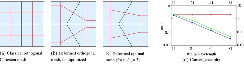
is equal to five periods of the wave. The permittivity tensor is assumed to be diagonalε= Diag(εx, εy). The Cartesian barycentric grid as depicted in Fig. 1(a) is well-suited for this exemplary problem. However, in traditional FIT the skew edges of a deformed grid, Fig. 1(b), lead to non-diagonal entries in the material matrix as explained in Section 4.3. Disregarding these entries endangers stability and convergence of the scheme. The red line in Fig. 1(d) shows that the numerical solution does not converge to the exact one in the case of orthogonal dual, where non-diagonal entries inM have been neglected. In our proposed approach, where the dual mesh is adapted to the material property, the convergence of the scheme is conserved, while keeping material matrices diagonal, as can be seen from the green line in Fig. 1(d). For comparison, the convergence of the traditional 2D FIT is plotted with blue line.
11 21 41 81
0.01 0.1 1
10 11 21 41 81
#cells/wavelength
error
(a) (b) (c)
(d)
0.01 0.1 1 10
Convergence plot Classical orthogonal
Cartesian mesh
Deformed orthogonal mesh, not optimized
Deformed optimal mesh (for ε x/ε y= 3)
Figure 1. From left to right: conversion plots for (a) classical orthogonal FIT, (b) deformed orthogonal, (c) optimal (forεx/εy = 3) mesh pairs. Black and red lines represent primal and dual mesh, respectively. Figure (d) shows the convergence plot for ε= Diag(100,1) and diagonal material matrices: Cartesian mesh (blue), deformed orthogonal (red) and deformed optimal (green). The error is defined as the relative error with respect to the analytic reference solution.
In 2D case the condition in Eq. (48) reduces to
pj =αεj(nj), (57) wherepj is a vector representing a primal edge andnj is a vector normal (in Euclidean sense) to the dual edge. An exemplary mesh pair satisfying this condition is found analytically as depicted in Fig. 1(c).
Let us define the simulation error as a relative error of the line integrated electric field strength in the discrete2 vector norm and ∞ in time with respect to the analytic reference solution
error := max
t∈T |
e−e
a|2/maxt∈T |ea|2, (58)
wheree, see Eq. (38), is a vector composed of electric degrees of freedom at timet=iΔt, i.e.,
fj+ine =
(i+1/2)Δt
(i−1/2)Δt e
j(t)dt, (59)
ne is number of edges, eais calculated from the exact solution and | · |2 is the2-norm.
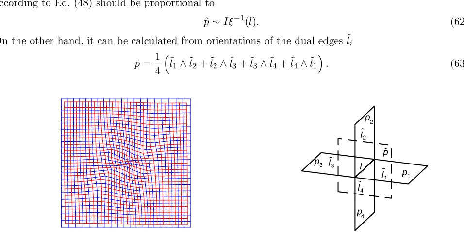
We have considered the example whereε= const. because in this case the exact solution is known and traditional FIT approach works well. This made comparison of numerical solutions transparent. However, the idea of mesh optimization is by no means restricted to homogenous materials. For example in Fig. 2(a) we present a mesh pair obtained by numerical optimization for
ε=
1 εxy(x, y)
εxy(x, y) 1
, with εxy(x, y) =
1 2−
|y|
ly
sin
π lx
x+lx 2
if |x| ≤ lx 2
0 if |x|> lx
2
, (60)
6. 3D CONSIDERATIONS
In 3D we first need to check when the set of conditions in Eq. (48) can be fulfilled by a mesh pair. For simplicity we assume that the material properties are constantξ = const. and therefore no averaging is needed, i.e., ξ =ξ. We also assume that the material relations are given by (17) and (18) from which follows that the material mappingξis self-conjugate, i.e.,ξ†=ξ. A proportionality relation∼is defined as
a∼b⇔a=αb, (61)
where α ∈R is the proportionality factor. As a possible constraint we consider an exemplary primal edge l and its dual facet ˜p, see Fig. 2(b). On the one hand, the mean orientation of the dual facet according to Eq. (48) should be proportional to
˜
p∼Iξ−1(l). (62)
On the other hand, it can be calculated from orientations of the dual edges ˜li
˜
p= 1 4
˜
l1∧˜l2+ ˜l2∧˜l3+ ˜l3∧˜l4+ ˜l4∧˜l1
. (63)
p1
˜
l1
p3 l˜3
p
2
˜
l2
p4
˜
l4
l
˜
p
(a)The optimized mesh for continuous but not constant ε(x, y). (b) Blue lines represent the primal mesh and the red ones the dual one.
Primal edge l and its dual facet p. Depicted are also neighbouring facets p and their dual edges l .
˜ ˜
i i
Figure 2. (a) Optimization mesh and (b) image visualizing the relation of primary edges and dual facets.
Let us suppose that the edge l is one of the x-edges of the Cartesian grid. Since ξ is constant it follows thatl1 ∼l3 and l2 ∼l4. It simplifies the expression for the mean orientation
˜
p∼˜l1∧˜l2, (64)
where ˜l1 and ˜l2 according to (48) are proportional to
˜
l1∼Iξ−1(p1) = Iξ−1(Iσz) =−μzaσa (65)
˜
l2∼Iξ−1(p2) = Iξ−1(Iσy) =−μyaσa. (66)
From which follows that the left-hand side of Eq. (62) is
˜
p∼μzbμycσb∧σc. (67) Expanding right-hand side of Eq. (62) gives
˜
p∼Iξ−1(l) =Iε−1xaσa. (68) Using the identity
where abc is a permutation symbol: abc = +1 if {a, b, c} is an even permutation of {1,2,3}, and abc=−1 if{a, b, c} is an odd permutation of {1,2,3}. We obtain from Eq. (62)
Iε−1xaσa∼μzbμycabcIσa, (70)
which simplifies to
ε−1xa =αμzbμycabc=−ανxa. (71) Repeating the same reasoning for y and z edges and using the symmetry of εand μ we arrive at the sufficient condition
ε=αμ, (72)
which guarantees constructing the optimal primal/dual mesh pair. Please note that Eq. (72) states that
εandμmust have not only the same main axes, but also the same eigenvalues associated with the main axes. The condition is not necessary. For example, in the case when the Cartesian grid axes are chosen as main axes of εandμ, i.e., whenεand μare diagonal, the condition from above is relaxed, i.e., both
εand μmay have arbitrary entries (eigenvalues) on their diagonals.
The condition in Eq. (72) has been derived for the Cartesian grid and flat facets of the dual mesh. One may wonder whether this result holds for other mesh pairs. From Eq. (48) it follows that
ξj
IWj
Wj
2 = 0 and
ξj
IWj
Wj
4 = 0. (73)
Noting that ξj(IWj)Wj4 is non-zero only for rather extraordinary and pathological choices of the
primal/dual mesh, we require that only Eq. (73)-left is satisfied.
We explore Eq. (73)-left on a deformed FIT mesh, i.e., we allow primal and dual nodes to move while keeping the connectivity. In this case Eq. (73)-left is an overdetermined system of nonlinear equations whose variables are positions of the primal/dual nodes. We form a goal function
K =
j
ξj
IWj
Wj
2
2 (74)
and look for its minimum. According to our investigations if Eq. (72) is satisfied the obtained minimum is zero, i.e., all equations of the overdetermined system are simultaneously solved. Moreover, if Eq. (72) is violated then the obtained minimum is greater than zero showing that not all of Eq. (73)-left can be solved simultaneously. This is in agreement with our predictions derived in the case of Cartesian primal mesh. Since we have not found any counterexample, i.e., the mesh pair for whichK = 0, and Eq. (72) is violated, we expect Eq. (72) to hold for arbitrary meshes and only relaxed if we use Cartesian grid with axes aligned to the main axes ofεand μ.
7. CONCLUSION
The classical orthogonal FIT mesh pair is a proper choice for scalar and diagonal material tensors. However, in the case of deformed primal grids, the orthogonal dual results in diagonal material matrices only for scalar material coefficients. When ε is a tensor and non-diagonal entries in material matrix are disregarded, the convergence is lost. However, adapting the dual mesh according to our criterion fixes the problem and allows to treat arbitrary material tensor consistently. In 3D setting, we have shown that the permittivity tensor being proportional to the permeability tensor implies existence of the mesh pair guaranteeing diagonal material matrices. However, proportionality of material tensors is very restrictive for physical applications.
ACKNOWLEDGMENT
REFERENCES
1. Doran, C. and A. Lasenby, Geometric Algebra for Physicists, 2nd Edition, Cambridge University Press, Cambridge, 2003.
2. Klimek, M., U. Roemer, S. Schoeps, and T. Weiland, “Space-time discretization of Maxwell’s equations in the setting of geometric algebra,” IEEE Proceedings of 2013 URSI International Symposium on Electromagnetic Theory (EMTS), 1101–1104, 2013.
3. Tonti, E., “Finite formulation of the electromagnetic field,”Progress In Electromagnetics Research, Vol. 32, 1–44, 2001.
4. Weiland, T., “Time domain electromagnetic field computation with finite difference methods,” International Journal of Numerical Modelling, Vol. 9, 295–319, 1996.
5. Sobczyk, G., “Simplicial calculus with geometric algebra,”Clifford Algebras and Their Applications in Mathematical Physics, 279–292, Springer, 2011.
6. Hestenes, D., “Differential forms in geometric calculus,” Clifford Algebras and their Applications in Mathematical Physics, 269–285, Springer, 1993.
7. Mullen, P., P. Memari, F. de Goes, and M. Desbrun, “HOT: Hodge-optimized triangulations,” ACM Trans. Graph. Vol. 30, 103:1–103:12, 2011.
8. Bellver-Cebreros, C. and M. Rodriguez-Danta, “An alternative model for wave propagation in anisotropic impedance-matched metamaterials,” Progress In Electromagnetics Research, Vol. 141, 149–160, 2013.
9. Lindell, I. V., “Electromagnetic wave equation in differential-form representation,” Progress In Electromagnetics Research, Vol. 54, 321–333, 2005.