A New Planar Electromagnetic Levitation System Improvement
Method Based on SIMLAB Platform in Real Time Operation
Mundher H. A. Yaseen1, * and Haider J. Abd2
Abstract—Electromagnetic levitation system is commonly used in the field of magnetic levitation system train. Magnetic levitation technology is one of the most promised issue of transportation and precision engineering. Magnetic levitation systems are free of problems caused by friction, wear, sealing and lubrication. In this paper, a new prototype of the magnetic levitation system is proposed, designed and successfully tested via SIMLAB platform in real time. In addition, the proposed system was implemented with an efficient controller, which is linear-quadratic regulator (LQR) and compared with a classical controller which is proportional-integral-derivative (PID). The present system has been tested with two different criteria: signal test and load test under different input signals which are Sine wave and Squar wave. The findings prove that the suggested levitation system reveals a better performance than conventional one. Moreover, the LQR controller produced a great stability and optimal response compared to PID controller used at same system parameters.
1. INTRODUCTION
Magnetic levitation technology is a perfect solution to achieve better performance for many motion systems, e.g., precision positioning, manipulation, suspension, and haptic interaction due to its non-contact, non-contamination, multi-Degrees-Of-Freedom (DOF), and long-stroke characteristics [1– 4]. Recently, the research on magnetic levitation attracts many researchers, and various types of magnetically levitated (maglev) motion systems are proposed. Generally, these maglev motion systems are realized using either Lorentz force or electromagnetic force, and both the moving magnet design and moving-coil design are proposed for applications with different requirements.
In literature, different methods and models are suggested to develop electromagnetic levitation systems and improve the system response [5–17]. However, most of the contributions require data from measurement devices or observer algorithms. The position and electric current state data are taken from related measurement devices, but for velocity state data, an observer should be synthesized to estimate the unavailable signal of the nonlinear dynamical system. Furthermore, it needs a complex system design and is not cost efficient. In this paper, a new technique is proposed to develop the control system based on a plate maglev system with the mathematical model. The new system uses a SIMLAB platform to control the position of electromagnetically levitated system in real time via Matlab/Simulink environment.
2. MAGLEV SYSTEM CONSTRUCTION
In this section, firstly, the construction of the magnetic levitation system and its components will be explained.
Received 13 September 2017, Accepted 31 October 2017, Scheduled 29 November 2017
* Corresponding author: Mundher H. A. Yaseen ([email protected]).
Levitation system or maglev is a method by which an object is suspended with no support other than magnetic fields. Magnetic force is used to counteract the effects of the gravitational acceleration and any other acceleration. The two primary issues involved in magnetic levitation are lifting forces: providing an upward force sufficient to counteract gravity and stability: ensuring that the system does not spontaneously slide or flip into a configuration where the lift is neutralized. Maglev trains perform three different parts to operate in high speeds which are: Levitation, Propulsion and Guidance. This paper focus on the levitation system part.
The proposed experimental magnetic levitation system is shown in Figure 1. The system is made up 4 electromagnets as actuators for applying magnetic forces to achieve stable levitation and precise position control, a rigid square plate with 4 permanent magnets on each corner, and 4 Hall effect sensors for sensing the position of the levitating plate, andV a is coil applied voltage.
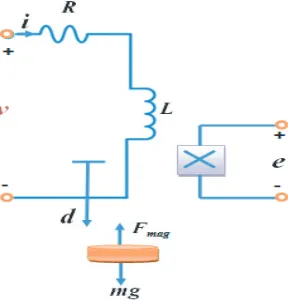
Figure 1. Free body diagram of magnetic levitation system.
The electromagnets are 15 mH solenoid coils with 2 Ω internal resistances. The Hall effect sensors are linear ratiometric Hall effect sensors with 50 V/T. The permanent magnets are N52 neodymium disc magnets with 12.70 mm diameter and 6.35 mm thickness. The plate is a transparent acrylic plate with 152.4 mm×152.4 mm×3.175 mm. The frame is constructed by wood. For simplicity and tractability, the system is modeled using a quarter of the system (similar to a quarter car model). The model of the quarter-system is shown in Figure 2, whereR is the resistance of the coil, Lthe inductance of the coil, v the voltage across the electromagnet, i the current through the electromagnet, m the mass of the levitating magnet plus one-forth of the mass of the acrylic plate, g the acceleration due to gravity,
dthe vertical position of the levitating magnet measured from the bottom of the electromagnet, Fmag
the force on the levitating magnet generated by the electromagnet, and ethe voltage across the Hall effect sensor.
3. CASE STUDY
In this section, the mathematical model of maglev system is presented, and the force actuated by the electromagnet is formulated as [18]
Fmag=C
i(t)
Figure 2. Electromagnetic levitation system model.
where (t) denotes the current across the electromagnet,dthe vertical position, andC a constant related to turn ratio and cross sectional area of the electromagnet. From a force balancing equation, we have
md¨=mg−Ci(t)
d3 (2)
wherem is the mass of the levitating magnet plus one-fourth of the mass of the acrylic plate andg the acceleration due to gravity.
In addition, an electrical relation of the voltage supply and the electromagnetic coil can be expressed by
v(t) =R·i(t) +Ldi
dt (3)
whereR and L are the resistance and inductance of the electromagnet, respectively. Now consider the following perturbations with respect to the change of them
i(t) =i0+ Δi(t)
d(t) =d0+ Δd(t)
v(t) =v0+ Δv(t)
(4)
wherevo is the required equilibrium coil voltage to suspend the levitating plate atdo.
Under this perturbation, the dynamics in Eqs. (2) and (3) around an operating point (i0, d0, v0) can be linearized
mĨd =
3Ci0
d4 0
Δd−
C d3 0
Δi (5)
˙
Δi = −R
LΔi−
1
LΔv (6)
where Δi, Δv, Δdare linearization of the system about the equilibrium point. After eliminating Δiin Eq. (6) and applying Laplace transforms, we obtain the transfer function from Δv to Δdgiven as
ΔD(s) ΔV(s) =
−gR
v0
(Ls+R)
s2−3Ci0
md4 0
(7)
where ΔV(s) and ΔD(s) denote the Laplace transforms of Δv(t)) and Δd(t), respectively. Hall sensor has an output voltage of the given form [19]
e(t) =α+ β
whereα, β, γ are constant sensor parameters. A linearization of Eq. (8) arounde(t) =e0+Δeresults in
Δe=−2β
d3 0
Δd+γΔi (9)
where Δeis the sensor voltage.
Applying Laplace transform to Eq. (9) and using I(s) = ΔV(s)/(Ls+R) from Eq. (3) and the representation in Eq. (7), we obtain a relation between the electromagnet voltage ΔV(s) and a sensor voltage perturbation ΔE(s) as follows;
ΔE(s) ΔV(s) =
γ
s2−3Ci0
md40
+2βRC
md60
(Ls+R)
s2−3Ci0
md40
(10)
Equation (10) can be represented also in the state space form after applying the second derivative of Eq. (5) and first derivative of Eq. (6). Thus, the state space representation of the linearized model of Equation (10) can be represented by followings:
x˙ 1 ˙ x2 ˙ x3 = ⎡ ⎢ ⎢ ⎢ ⎢ ⎣
0 1 0
3C
m i0
d40 0 − C m
1
d30
0 0 −R
L ⎤ ⎥ ⎥ ⎥ ⎥ ⎦ x 1 x2 x3 + ⎡ ⎢ ⎣ 0 0 1 L ⎤ ⎥
⎦u (11)
y =
−2β
d3 0 γ
x1
x2
x3
(12)
The measured output system (y) can be obtained by simplified Equation (9), where Δe=y, Δd=x1, and Δi=x3).
Suppose that x= [x1 x2 x3] = [dd i˙ ] is the state of the system, where dis the controlled output,
y=e the measured output, andu=v the control input.
By substituting system parameters in Table 1 into Eq. (10),
G(s)H(s) = 20.66s
2+ 61803
s3+ 132.5s2−1471s−194900 (13)
The numerical values of the state space equations are given below
x˙ 1 ˙ x2 ˙ x3 =
0 1 0
1471 0 −9.81
0 0 −133
x1 x2 x3 + 0 0 66.66
u (14)
y = [ −144 0 0.31 ]
x 1 x2 x3 (15)
4. CONTROLLER DESIGN
This section deals with the development of PID based control and LQR controller for magnetic levitation system
4.1. Linear Quadratic Regulator (LQR) Controller
The Linear Quadratic Regulator (LQR) method is similar to Root Locus approach by inserting the closed loop poles of the system into the desired location [20]. The EMS linearization dynamic model is formulated by state space as below:
˙
x(t) = Ax(t) +Bu(t) (16)
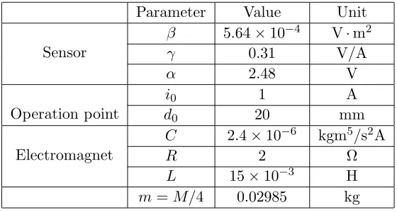
Table 1. Proposed system parameter.
Parameter Value Unit
Sensor
β 5.64×10⁻⁴ V·m2
γ 0.31 V/A
α 2.48 V
Operation point
i0 1 A
d0 20 mm
Electromagnet
C 2.4×10⁻⁶ kgm5/s2A
R 2 Ω
L 15×10−3 H
m=M/4 0.02985 kg
Thex(t) state can be measured, and the cost function of constructing controller can be minimized based on the formula below:
J(u) = +∞
0
xT (t)Qx(t) +uT(t)Ru(t)dt (18)
whereQandRvalues can be considered positive definite weighting matrices. For initial state condition, the variablex(0) is considered as a steady state based on perturbation of the control system. The first term of the J(u) function is considered as cost subject which is assigned to the energy intransient response.
The control signal u(t) is considered as linearly proportional to the specified air gap. It is also proportional to the clearance of track boundary condition at desired operating point (io, zo) in design
stage.
Using the linear state feedback can be expressed by the equation below
u(t) =−[kp(x1(t)−zref) +kv(x2(t)) +ka(x3(t)) (19)
wherekp is the steady error,kv the control suspension damping, and ka taken for all stability margins.
The linear controller limitations are considered as the ability to suppress disturbances in the control loop. The calculated LQR gains are [kp = 32483, kv = 90.4, ka =−9.4].
4.2. PID Controller
The schematic diagram of PID controller is given in Figure 3. This control system is working based on the calculations of the error value, trying to reduce the error percentage by adjusting the controller parameters. The general form of this controller is formulated as below [20].
u(t) =Kp ⎛
⎝e(t) + 1
Ti t
0
e(τ)dτ+Td
de(t)
dt
⎞
⎠ (20)
whereu(t) denotes the control signal, Kp the proportional gain, Ti the integral time, Td the derivative
time, ande(t) the difference between the reference point and the actual plant output. Kp,Ti andTdare
tuned for better control operation. By placing the closed loop poles at P = [−132.45 38.36 −28.36], the calculated PID gains are [Kp = 10, Ki = 4, Kd= 0.2].
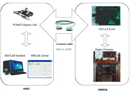
5. PROPOSED SYSTEM DESIGN AND HARDWARE CONTROL UNIT
Figure 3. Block diagram of PID controller.
Figure 4. Component of the maglev prototype system.
will be connected with both of the maglev prototype and the MATLAB Simulink which enables the system to control and operate. Proximity sensors are specific devices that enable the measurement of the air gap distance. There are many types of sensors such as laser, inductive, resistive, hall-effect and IR sensors. In the present system, the Hall-effect sensor is used to detect the distance of air gap. The sensor position in the present maglev system is at the bottom of the coil. The unique feature of this type of sensors encourages the researchers and producers to use it in many fields such as aircrafts, automobile and medical machines.
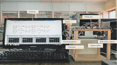
5.1. Experimental Results and Discussion
Figure 5. System implementation.
maglev system which represents the access point to maglev train. The results can be classified into two cases of test: signal representation test and load representation test as follows.
5.1.1. Results of Signal Representation Test
The first group of tests is the input signal representation. Two kinds of standard signals have been applied: Sine wave and Square wave. The input signal test was done with variation of different tuning parameters as follows.
I. Effect on One Point
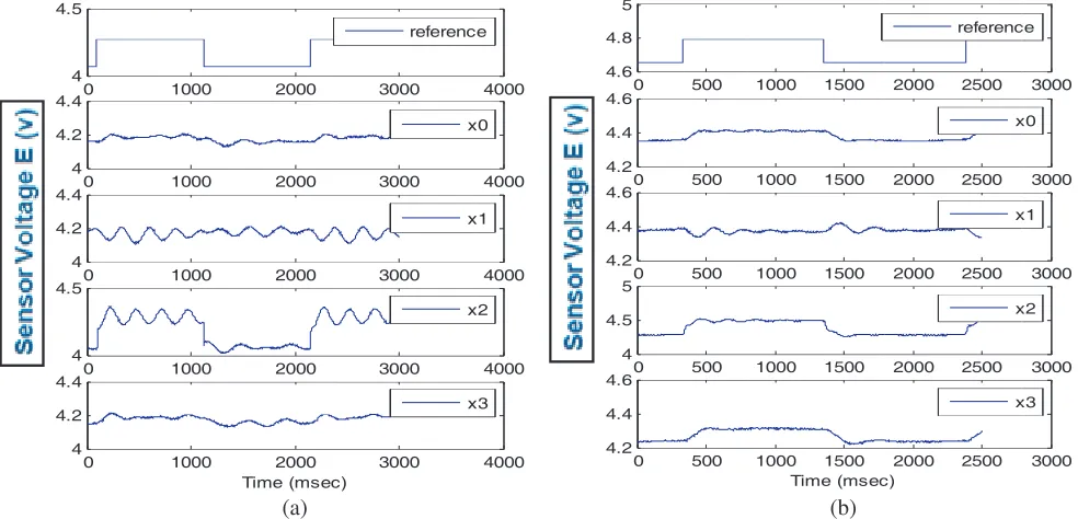
The input of Sine wave signal was applied on one single point in the prototype maglev plate. The benefit of this test is to show the effect of sudden changes in one point on the maglev plane. The test signals were implemented with two types of control systems, PID and LQR, and the results are shown in Figures 6(a)–(b), respectively.
From the results indicated in Figure 6, it is noticed that the system performance is stable, and the system responses are perfect. Furthermore, the signal response that points x and x3 respond based on the same input wave, while point x1 responds oppositely. In this case, the system is able to convert the force reaction and dynamic moment in the load points (i.e., the discs) based on the load variation in each point of the plane. Moreover, the experimental results showed that LQR controller had optimum response and better stability than PID controller under the effect of the same input signal and parameters.
4 4 4. 4 4. 4 A ir gap di s tanc e 4 4 4. 4 0 100 4 4.5 0 100 4.1 15 4.2 0 100 15 4.2 0 100 4 4.5 0 100 4.1 15 4.2 00 2000 00 2000 00 2000 00 2000 00 2000 Time (msec 3000 referen 3000 3000 3000 3000 c) 4000 nce 4000 x0 4000 x1 4000 x2 4000 x3 A ir gap di s ta n c e 0 500 4.5 5 0 500 4.2 4.4 4.6 0 500 4.35 4.4 4.45 0 500 4 4.5 5 0 500 4.2 4.4 4.6 1000 1500 1000 1500 1000 1500 1000 1500 1000 1500 Time (mse 2000 2500 referen 2000 2500 2000 2500 2000 2500 2000 2500 ec) 3000 ce 3000 x0 3000 x1 3000 x2 3000 x3 (a) (b)
Figure 6. Sine wave signal applied on one single using (a) PID and (b) LQR controller.
4 4 4 4 4 4 4 4 0 100 4 4.5 0 100 4 4.2 4.4 0 100 4 4.2 4.4 0 100 4 4.5 0 100 4 4.2 4.4 00 2000 00 2000 00 2000 00 2000 00 2000 Time (msec 3000 referenc 3000 x 3000 x 3000 x 3000 c) x 4000 ce 4000 x0 4000 x1 4000 x2 4000 x3 4 4 4 4 4 4 4 4 A ir g ap di s ta n c e ( v ) 4 4 4 4 0 500 4.6 4.8 5 0 500 4.2 4.4 4.6 0 500 4.2 4.4 4.6 0 500 4 4.5 5 0 500 4.2 4.4 4.6 1000 1500 1000 1500 1000 1500 1000 1500 1000 1500 Time (msec 2000 2500 referenc 2000 2500 x 2000 2500 x 2000 2500 x 2000 2500 c) x 3000 ce 3000 x0 3000 x1 3000 x2 3000 x3 (a) (b)
Figure 7. Square wave signal applied on one single using (a) PID and (b) LQR controller.
From all the results using (single point effect), it can be seen that Sine wave signal revealed better performance than square wave signal in both stability and response.
5.1.2. Results of Load Representation Test
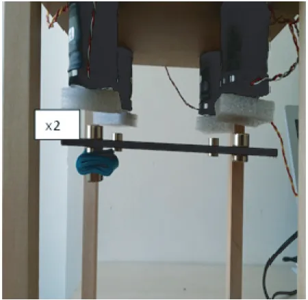
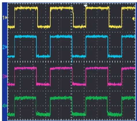
Figure 8. Load test applied (one point). Figure 9. PWM results of load test applied one single point.
Opp
Load point (x2
posite point (x1
(x0
(x3
PWM
)
) 0)
)
"
width
Load cha effec
ange ct
Figure 10. PWM comparative of coil voltage response.
plane load of the maglev system plate which represents the whole system.
I. Case One: Effect on One Point
In this case, the input actual load of 10 grams is applied on one single point in the prototype maglev plate. The reason of applying this test is to investigate the effect of unbalance change of load in the plate based on one point of maglev plane. The test applied on point x2 is as shown in Figure 8.
The load test is done with LQR control system, and the results are presented in Figure 9. The results indicate that the system is stable, and the system responds perfectly. It is clear from the pulse width modulation (PWM) results that the controller power supply of the present maglev system responds significantly as shown in Figure 10. It is seen that the average value of the voltage fed to the coils differs from point x2 which represents the load input point and point x1 which represents the opposite side point.
II. Case Two: Effect on Three Point (Plane)
Figure 11. Suspended load on the system plate. Figure 12. PWM results of load applied on a plane.
The test load is applied using the LQR control system as presented before, as shown in Figure 12. From this result it can be observed that the system ability to deal with the force reaction and the dynamic moment in the load line is based on the load variation in four points of the plane.
It is clear from the pulse width modulation (PWM) results that the control power supply of the present maglev system responds significantly. Also, the system responds homogeneously, and all points respond based on the same input load at the same time of sequence. It means that the system is able to deal with the force reaction and the dynamic moment of the plane.
6. CONCLUSION
In this paper, an efficient technique of magnetic levitation system is proposed and successfully tested based on SIMLAB platform in real time operation. Furthermore, the proposed system was described mathematically and implemented practically under different tests and parameters. The present levitation system was implemented with modern controller which is LQR controller and compared with classical controller like PID controller under the same tuning parameters. Moreover, the proposed system has been examined under two tests: signal test and load test. The findings show that the LQR controller revealed a significant improvement in system performance. It was observed that LQR controller offered notable stability and better response than PID controller at the same input parameters.
REFERENCES
1. Ono, M., S. Koga, and H. Ohtsuki, “Japan’s superconducting Maglev train,”IEEE Instrum. Meas. Mag., Vol. 5, No. 1, 9–15, 2002.
2. Chen, M.-Y., M.-J. Wang, and L.-C. Fu, “A novel dual-axis repulsive maglev guiding system with permanent magnet: Modeling and controller design,” IEEE/ASME Trans. Mechatron., Vol. 8, No. 1, 77–86, 2003.
3. De Boeij, J., M. Steinbuch, and H. Gutierrez, “Real-time control of the 3-DOFsled dynamics of a null-flux Maglev system with a passive sled,”IEEE Trans. Magn., Vol. 42, No. 5, 1604–1610, 2006. 4. Rote, D. and Y. Cai, “Review of dynamic stability of repulsive-force maglev suspension systems,”
5. Banerjee, S., D. Prasad, and J. Pal, “Design, implementation, and testing of a single axis levitation system for the suspension of a platform,”ISA Trans., Vol. 46, No. 2, 239–246, 2007.
6. Lee, Y., J. Yang, and S. Shim, “A new model of magnetic force in magnetic levitation systems,”
J. Electr. Eng. . . ., Vol. 3, No. 4, 584–592, 2008.
7. Khemissi, Y., “Control using sliding mode of the magnetic suspension system,” International Journal of Electrical & Computer Sciences, No. 3, 1–5, 2010.
8. Liu, C. and J. Zhang, “Design of second-order sliding mode controller for electromagnetic levitation grip used in CNC,”Proc. 2012 24th Chinese Control Decis. Conf. CCDC 2012, Vol. 2, No. 1, 3282– 3285, 2012.
9. Xing, F., B. Kou, C. Zhang, Y. Zhou, and L. Zhang, “Levitation force control of maglev permanent synchronous planar motor based on multivariable feedback linearization method,” 2014 17th International Conference on Electrical Machines and Systems (ICEMS), 1318–1321, 2014.
10. Zhu, H., T. J. Teo, and C. K. Pang, “Design and modeling of a six-degree-of-freedom magnetically levitated positioner using square coils and 1-D Halbach arrays,”IEEE Trans. Ind. Electron., Vol. 64, No. 1, 440–450, 2017.
11. Vinodh Kumar, E. and J. Jerome, “LQR based optimal tuning of PID controller for trajectory tracking of magnetic levitation system,”Procedia Eng., Vol. 64, 254–264, 2013.
12. Hussein, B., N. Sulaiman, R. Raja Ahmad, M. Marhaban, and H. Ali, H infinity controller design to control the single axis magnetic levitation system with parametric uncertainty,” J. Appl. Sci., Vol. 11, No. 1, 66–75, 2011.
13. Cho, J. and Y. Kim, “Design of levitation controller with optimal fuzzy PID controller for magnetic levitation system,”J. Korean Inst. Intell. Syst., Vol. 24, No. 3, 279–284, 2014.
14. Zhang, Y., Z. Zheng, J. Zhang, and L. Yin, “Research on PID controller in active magnetic levitation based on particle swarm optimization algorithm,”Open Automation &Control Systems Journal, Vol. 7, No. 1, 1870–1874, 2015.
15. Uroˇs, S., A. Sarjaˇs, A. Chowdhury, and R. Sveˇcko, “Improved adaptive fuzzy back stepping control of a magnetic levitation system based on symbiotic organism search,” Applied Soft Computing, Vol. 56, 19–33, 2017.
16. Hong, D.-K., B.-C. Woo, D.-H. Koo, and K.-C. Lee, “Electromagnet weight reduction in a magnetic levitation system for contactless delivery applications,” Sensors, Vol. 10, 6718–6729, 2010.
17. Li, J.-H. and J.-S. Chiou, “Digital control analysis and design of a field-sensed magnetic suspension system,” Sensors, Vol. 15, 6174–6195, 2015.
18. Cheng, D. K.,Field and Wave Electromagnetics, Addison-Wesley, MA, 1983. 19. Smaili, A. and F. Mrad, Applied Mechatronics, Oxford, MA, 2008.