Scholarship@Western
Scholarship@Western
Electronic Thesis and Dissertation Repository
8-29-2016 12:00 AM
Estimation of Wind Hazard over Canada and Reliability-based
Estimation of Wind Hazard over Canada and Reliability-based
Assignment of Design Wind Load
Assignment of Design Wind Load
Qian Tang
The University of Western Ontario Supervisor
Hanping Hong
The University of Western Ontario
Graduate Program in Civil and Environmental Engineering
A thesis submitted in partial fulfillment of the requirements for the degree in Master of Engineering Science
© Qian Tang 2016
Follow this and additional works at: https://ir.lib.uwo.ca/etd
Part of the Civil and Environmental Engineering Commons
Recommended Citation Recommended Citation
Tang, Qian, "Estimation of Wind Hazard over Canada and Reliability-based Assignment of Design Wind Load" (2016). Electronic Thesis and Dissertation Repository. 4092.
https://ir.lib.uwo.ca/etd/4092
This Dissertation/Thesis is brought to you for free and open access by Scholarship@Western. It has been accepted for inclusion in Electronic Thesis and Dissertation Repository by an authorized administrator of
i
Abstract
The current National Building Code of Canada (NBCC) recommends a wind load factor of 1.4
and the nominal wind velocity pressure corresponding to a 50-year return period value of the
annual maximum hourly-mean wind speed, VAH. This study is focused on mapping wind hazard
for Canada and on calibrating the required design wind load to improve reliability consistency of
designed structures.
Extreme value analysis of VAH was carried out by considering surface wind observations from
approximately 1300 stations. The results indicate that the spatial trends of the estimated mean of
VAH are similar whether the data from stations with at least 20 or 10 years’ useable wind
observations are considered, but the small sample size affects the spatial variations of the
coefficient of variation (cov) of VAH. The estimated 50-year return period values of VAH based on
the at-site analysis differ from those inferred from two previous versions of the NBCC, and the
differences persist if the estimates were obtained by using the region of influence approach.
Potential reasons for the discrepancy were elaborated.
It was shown that an improved reliability consistency can be achieved if a wind load factor of
1.0 is employed and the nominal wind velocity pressure is assigned using the 500-year return
period value of VAH. It is also shown that a further improvement of the reliability consistency can
be achieved if a variable return period as a function of cov of VAH is used to assign the nominal
wind velocity pressure.
Keywords: Annual maximum wind speed, Code calibration, Design code, Design wind velocity
pressure, Extreme value analysis, Reliability analysis, Target reliability index, Wind hazard
ii
Acknowledgements
First and foremost, I would like to express my sincere gratitude to my supervisor, Dr. Hanping
Hong for his advice on my thesis work. This thesis could not be completed without his guidance.
His attitude towards research is contagious and inspiring.
I want to thank my colleagues, Shucheng Yang, Qian Huang, Jiyang Gu and Chao Feng for
providing suggestion and comments on my thesis and my graduate studies. Special thanks to Drs.
Sihan Li and Wei Ye for teaching and helping me with data process and data mapping tasks.
Collaboration from Mr. P. Hong for Chapter 3 is appreciated and acknowledged.
Many thanks go to Dr. Newson, Dr. Wang, and Dr. Zhou for reading my thesis and providing
constructive comments and suggestions.
Lastly, I am deeply and forever indebted to my parents for their love, support and
iii
Table of Contents
Abstract ... i
Acknowledgements ... ii
List of Tables ... v
List of Figures ... vi
List of Symbols and Abbreviations... x
Chapter 1 Introduction ... 1
1.1 Introduction and background ... 1
1.2 Research objectives and thesis outline ... 5
Reference ... 6
Chapter 2 At-site Analysis and Regional of Influence ... 8
2.1 Introduction ... 8
2.2 Surface wind observations ... 12
2.3 Extreme value analysis approach: at-site and regional approaches ... 15
2.4 Wind hazard estimation and mapping... 21
2.4.1 Wind hazard mapping based on extreme wind speed inferred from the NBCC ... 21
2.4.2 Comparison of the spatial varying wind hazard using data with nA ≥ 20 and ≥ 10 ... 22
2.4.3 Estimated wind hazard using the ROI approach ... 28
2.5 Effect of additional considerations on spatially interpolated wind hazard maps... 32
2.6 Summary and conclusions ... 37
iv
Chapter 3 Codification of Wind Load for Improved Reliability Consistency over Canadian Sites
... 42
3.1 Introduction ... 42
3.2 Probabilistic models adopted for the calibration ... 44
3.3 Calibrating design wind load for spatially varying extreme wind characteristics ... 48
3.3.1 Limit state function and analysis procedure ... 48
3.3.2 Calibration results and wind speed contour map for reliability consistent design ... 49
3.4 Conclusions ... 53
References ... 54
Chapter 4 Conclusions and Recommendations for future work ... 56
4.1 Summary and conclusions ... 56
4.2 Recommendations for future work ... 58
Appendix A. Spatially Interpolated Statistics of Annual Maximum Wind Based on Ordinary Kriging with Nugget Equal to Zero ... 59
Appendix B. Interpolated 50-year Return Period Values for Specified Locations in NBCC Based on At-site Analysis and ROI ... 64
v
List of Tables
Chapter 2
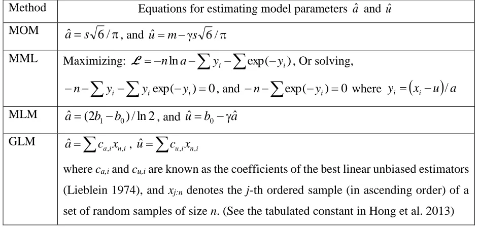
Table 2-1. Methods for estimating the model parameters and quantiles based on the Gumbel
model (for n samples, with sample mean m and sample standard deviation s). ... 17
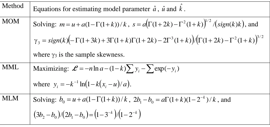
Table 2-2. Methods for estimating the model parameters and quantiles based on the generalized
extreme value distribution... 18
Table 2-3. Equations used to calculate L-moment ratios t iand t3i for Ri. (Burn 1990). ... 20
Appendix B
Table B1. Comparison of NBCC-2005, NBCC-2010 and interpolated 50-year return period
vi
List of Figures
Chapter 2
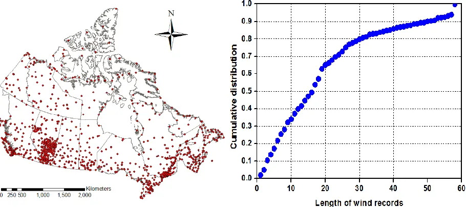
Figure 2-1. Locations of the meteorological stations where wind speed records are available in
EC HLY01 digital archive, and empirical cumulative distribution of the length of wind
measurement period at each station: a) Spatial distribution of the stations, b) Empirical
cumulative distribution of length of wind measurement period. ... 13
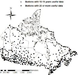
Figure 2-2. Locations of 583 stations with useable data used in this study. ... 15
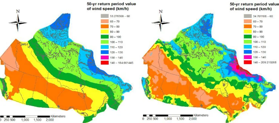
Figure 2-3. Wind hazard maps inferred from the reference velocity wind pressures given in the NBCC-2005 and NBCC-2010. ... 22
Figure 2-4. Mean and coefficient of varaition of VAH for the case with nA≥ 20. ... 23
Figure 2-5. Mean and coefficient of varaition of VAH for the case with nA ≥ 10... 23
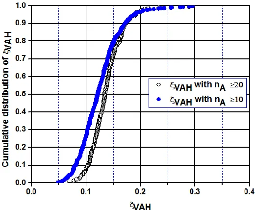
Figure 2-6. Empirical distribution of ξVAH ... 25
Figure 2-7. Comparison of the estimated vAH-50 by different fitting methods and considering VAH is Gumbel distributed: a) using the MOM vs using the GLM; b) using the MML vs using the GLM; c) using the MLM vs using the GLM. ... 25
Figure 2-8. Estimated vAH-50 using the GLM for the selected meteorological stations shown in Figure 2-2: a) Contour map of vAH-50 for the case with nA≥ 20, b) Contour map of vAH-50 for the case with nA≥ 10. ... 26
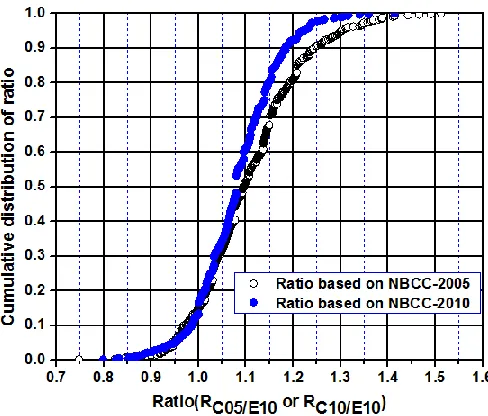
Figure 2-9. Empirical distribution of RC05/E10 and RC10/E10... 27
vii
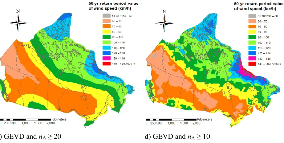
Figure 2-11. Wind hazard maps developed based on the ROI approach: a) Gumbel distribution
and nA≥ 20, b) Gumbel distribution and nA≥ 10, c) GEVD and nA≥ 20, d) GEVD and nA≥
10... 30
Figure 2-12. Wind hazard maps developed based on the ROI approach and consideing the
Gumbel model: a) vAH-100 for nA≥ 20, b) vAH-100 for nA≥ 10, c) vAH-500 for nA≥ 20, and d) v
AH-500 for nA≥ 10. ... 31
Figure 2-13. Trends of the 50-year return period values based on the adopted criteria and
applying the ordinary kriging technique without/with nugget equal to zero for the case with nA≥
20... 34
Figure 2-14. Trends of the 50-year return period values based on the adopted criteria and
applying the ordinary kriging technique without/with nugget equal to zero for the case with nA≥
10... 35
Figure 2-15. Statistics of the estimated ratio the 50-year wind speed by considering the values
inferred from the codes and the estimated values shown in Figure 2-13c and 2-14c: a) For the
case with nA≥ 20, b) For the case with nA≥ 10, c) For the case with nA≥ 20 & satisfy
Criterion 1, and d) For the case with nA≥ 10 & satisfy Criterion 1. ... 37
Chapter 3
Figure 3-1. Coefficient of variation of the annual maximum hourly-mean wind speed: a) for the
case with nA≥ 20 and b) for the case with nA≥ 10. ... 46
Figure 3-2. Voronoi polygon associated with each station for the estimation of area-weighted
viii
Figure 3-3. Mean and coefficient of variation of the annual maximum hourly-mean wind speed:
a) Mean of VAH (km/hr), and b) cov of of VAH (inferred from the analysis results obtained from
the ROI approach, see Chapter 2). ... 47
Figure 3-4. Estimated 50 and Pf for W = 1.40 and using T = 50 years to assigning the reference
wind velocity pressure: a) Estimated 50 and b) Estimated Pf. ... 50
Figure 3-5. Estimated 50 and Pf for W = 1.0 and using T = 500 years to assigning the reference
wind velocity pressure: a) Estimated 50 and b) Estimated Pf . ... 50
Figure 3-6. Estimated 50 and Pf for W=1.0and using the return period given in Eq. (3.5) to
assign vT: a) Estimated 50 and b) Estimated Pf . ... 51
Figure 3-7. Suggested design wind speed considering the return period shown in Eq. (3.5). .... 52
Figure 3-8. Ratio of factored design wind load to the suggested factored design wind load ... 53
Appendix A
Figure A1. Wind hazard maps inferred from the reference velocity wind pressures given in the
NBCC-2005 and NBCC-2010. ... 59
Figure A2. Mean and coefficient of varaition of VAH for the case with nA≥ 20. ... 60
Figure A3. Mean and coefficient of varaition of VAH for the case with nA≥ 10. ... 60
Figure A4. Estimated vAH-50 using the GLM for the selected meteorological stations shown in
Figure 2-2: a) Contour map of vAH-50 for the case with nA≥ 20, b) Contour map of vAH-50 for the
case with nA≥ 10. ... 61
Figure A5. Wind hazard maps developed based on the ROI approach: a) Gumbel distribution
and nA ≥ 20, b) Gumbel distribution and nA ≥ 10, c) GEVD and nA≥ 20, d) GEVD and nA≥
ix
Figure A6. Wind hazard maps developed based on the ROI apporach and consideing the
Gumbel model: a) vAH-100 for nA≥ 20, b) vAH-100 for nA≥ 10, c) vAH-500 for nA≥ 20, and d) v
x
List of Symbols and Abbreviations
vAH-50: 50-year return period value of annual maximum (hourly-mean) wind speed
nA: the number of years of useable wind measurements at a station
VAH: the annual maximum moving average (AMMA) of the hourly-mean wind
speed
vx: coefficient of variation of X
Dij: a distance to measure the closeness of the i-th and j-th stations in ROI
VAH: coefficient of variation of VAH
RC05/E10: the ratio of vAH-50 inferred from the NBCC-2005 to the estimated vAH-50 for the
case with nA ≥ 10
RC10/E10: the ratio of vAH-50 inferred from the NBCC-2010 to the estimated vAH-50 for the
case with nA ≥ 10
vLB: a lower bound of 77.55 km/h which is used in the NBCC-2010
50: reliability index for a service period of 50 years.
Pf : the probability of failure
vv: coefficient of variation of VAH
vT: the T-year return period value of VAH
W: the ratio of the wind load effect to the nominal wind load effect
Wn: the reference (or nominal) wind load effect on the structural member calculated
according to the design code
W: the wind load factor
D: the dead load factor
xi
RW/D: the ratio of the factored design wind load WWn to the factored design dead
load DDn
Rn: the nominal resistance
Dn: the nominal dead load
NBCC: National Building Code of Canada
AIC: Akaike Information Criterion
ROI: the region of influence
COV: coefficient of variation
RMSE: the root-mean-square-error
GEVD: the generalized extreme value distribution
GPD: the generalized Pareto distribution
MOM: the method of moments
MML: the method of the maximum likelihood
MLM: the method of L-moments
Chapter 1 Introduction
1.1 Introduction and background
The results of wind hazard assessment are used as the basis to assign wind load for design new
structures and assessing existing structures and infrastructure systems. Return period values of the
annual maximum hourly-mean wind speed, VAH, are employed to assign reference wind velocity
pressure in the National Building Code of Canada (NBCC). The T-year return period value of VAH
is defined as the value of VAH such that its corresponding probability of exceedance equals 1/T.
The wind velocity pressure is used to evaluate the design wind load according to
w e g p
pI qC C C (1.1)
here p is the specified external pressure caused by wind acted in a direction normal to the surface
of the structure (as a pressure directed towards or as a suction directed away from the surface), Iw
is the importance factor for wind load, q is the reference velocity pressure, Ce is the exposure
factor, Cg is the gust effect factor and Cp is the external pressure coefficient averaged over the area
of the surface considered.
The current NBCC recommends a wind load factor of 1.4 and the nominal wind velocity
pressure corresponding to 50-year return period value of VAH.
Some relevant information on the evaluation of the return period value of the annual maximum
wind speed can be found in Yip and Auld (1993), Yip et al. (1995), Morris (2009), and Hong et
al. (2014). Yip and Auld (1993) and Yip et al. (1995) described the update to the reference wind
pressures implemented in the NBCC-1995 (NRCC 1995). The Gumbel distribution was used to
they used wind records from 233 stations each with at least 10 years of data to estimate the
30-year return period value of the annual maximum wind speed by adopting the Gumbel model fitted
using the MOM. A wind hazard map was plotted based on the 30-year return period value of the
annual maximum wind speed estimated using the at-site statistics of the wind. The wind speeds
at locations tabulated in the NBCC were extracted from the map. To estimate extreme wind speed
for return period T other than 30 years, they introduced a ratio of the standard deviation to the
30-year return period value of the annual maximum wind speed, and assumed that the ratio can be
approximated by a constant for all stations considered. The error caused by using 30-year return
period values of the annual maximum wind speed and this constant ratio to estimate the return
period value other than 30 years (e.g., 10 and 100 years) depends on T and the actual statistics of
the annual maximum wind speed at a considered site (Hong et al. 2014).
Companion-action load combinations were adopted in the NBCC-2005 and the 50-year return
period value of the wind velocity pressure coupled with a wind load factor of 1.4 was
recommended in the NBCC-2005 (Bartlett et al. 2003a, b). The 50-year return period values of
the wind velocity pressure were calculated based on their corresponding 30-year values
recommended in the NBCC-1995 and by considering that the annual maximum wind speed is a
Gumbel variate. The reference wind velocity pressures were updated for the NBCC-2010 by
fitting the Gumbel distribution to the annual extreme wind speed using the MOM. For the
updating, it was assumed that a constant cov of the annual maximum wind speed equal to 0.124
could be adequate for all the meteorological stations considered (Morris 2009). A comparison of
the 50-year return period value of annual maximum (hourly-mean) wind speed, vAH-50, inferred
from the NBCC-2010 and NBCC-2005 (Hong et al. 2014) indicated that there are significant
decrease in the NBCC-2010 as compared to the NBCC-2005 is about 30%; the largest increase is
less than 10%; the majority of changes are within 10%; two relatively high wind regions in the
Northwest Territories and Nunavut in the NBCC-2005 are eliminated in the NBCC-2010; a series
of continuous “consistent” wind speed regions from east to west of the country shown in the wind
map inferred from the NBCC-2010 was not present in the map inferred from the NBCC-2005. It
was considered that these differences are partly due to the use of a constant cov to develop vAH-50
for the NBCC-2010.
A wind hazard mapping for Canada was carried out based on the annual maximum wind speed
from more than 230 stations, where at least 20 years of useable data are available from each station
(Hong et al. 2014). They also applied the Akaike Information Criterion (AIC) (Akaike 1974) and
concluded that the Gumbel distribution is preferable than the generalized extreme value
distribution (GEVD) for more than 70% of cases. The consideration of at least 20 years of useable
data was aimed at reducing the statistical uncertainty in the estimated wind hazard due to small
sample size, although it is inconsistent with the attitude taken in develop wind hazard for previous
versions of the code. The wind hazard maps in Hong et al. (2014) were developed based on the
at-site analysis results (i.e., results from the extreme value analysis of the annual maximum wind
speed at each meteorological station with suitable surface wind observations). It was shown that
there are discrepancies between their estimated vAH-50 and those inferred from the NBCC-2005 and
NBCC-2010. In an attempt to further investigate the wind hazard at Canadian sites and to further
reduce the effect of small sample size to estimate return period values of the annual maximum
wind speed, the use of regional frequency analysis (Hosking and Wallis 1997) for wind hazard
mapping was presented by Hong and Ye (2014). Comparison of the vAH-50 values estimated based
are in good agreement, especially if the Gumbel model is used. One of the major disadvantages
of using the wind records from a station with at least 20 years of useable data is that the valuable
information from a station with less than 20 years of useable data is neglected for wind hazard
mapping. Therefore, the density of the spatial distribution of the potentially available
meteorological stations with valuable wind records is reduced for wind hazard mapping. In
addition, it is unknown if the consideration of the stations, each with less than 20 years of useable
data, could affect the estimated return period value of the annual maximum wind speed in the
regional frequency analysis and wind hazard mapping.
It must be emphasized that the recommended wind load factor of 1.4 and the nominal wind
velocity pressure corresponding to 50-year return period value of the annual maximum
hourly-mean wind speed, VAH, in the NBCC (NRCC 2005, 2010) are calibrated based on a typical
coefficient of variation (cov) of VAH for a (50-year) target reliability index of 3.0 (i.e., failure
probability of 1.35×10⁻³) (Bartlett et al. 2003a, b) However, the cov of VAH is geographically
varying and ranges from 0.05 to 0.3; the reliability indices of the structures designed according to
the current code is sensitive to the cov of VAH at the construction site (Hong et al. 2016). This is
partly because the wind load is proportional to the square of VAH, resulting in that the cov of the
wind load equals about twice of the cov of VAH if all other variables involved in evaluating the
wind force are treated deterministically. Moreover, although the use of a specified return period
value of the wind velocity pressure and a calibrated wind load factor given a cov of VAH can lead
to a target reliability, such a set of specified values and wind load factors is not unique. In fact, if
the resulting factored design wind loads for different sets of specified values and wind load factors
are the same, the same target reliability can be achieved. In addition, it is noted that the
of 700 years for the strength design of Category II structures (Vickery et al. 2010; Cook et al.
2011).
The above background information raises questions as to whether the design wind load
requirements could be modified to improve the reliability consistency of codified design under
wind load.
1.2 Research objectives and thesis outline
There are two main objectives for the proposed study which are listed below:
1) Evaluate and map wind hazard for Canada using surface wind observations.
2) Calibrate required factored design wind load considering the geographically varying wind
climate (i.e., geographically varying coefficient of variation of the annual maximum
hourly-mean wind speed).
For the evaluation and mapping of wind hazard, surface wind observations from Environment
Canada for approximately 1300 stations are processed and adjusted by exposure and height. Data
from stations, each with at least 10 years of usable data are employed. The wind hazard assessment
was carried out using the at-site analysis and region of influence approach. For the analysis, only
the winds due to synoptic winds are considered; the winds caused by high intensity wind events
such as downbursts and tornados are excluded from the analysis. This is justified since the winds
due high intensity wind events are not considered in the current National Building Code of Canada.
For the calibration, the commonly employed first-order reliability method (Madsen et al. 2006)
is employed, and a selected target reliability index consistent with that used to develop current
design code is considered. The selected target reliability index is based on that employed to
this thesis are 1) developed Canadian wind hazard map based on at-site analysis and regional of
influence approach, and 2) calibrated the required design wind load that can be easily implemented
in the design code to achieve improved reliability consistency.
The tasks carried out to achieve the first objective are presented in Chapter 2, and those to
achieve the second objective are descried in Chapter 3. Finally, a summary of concluding remarks
is presented in Chapter 4. Also, some potential future studies are suggested.
Chapter 2 contains part of a manuscript (co-authored by H.P. Hong) to be submitted for possible
publication; Chapter 3 contains part of a manuscript (co-authored by P. Hong and H.P. Hong) to
be submitted for possible publication.
Reference
Akaike, H. 1974. A new look at the statistical model identification. IEEE Transactions on Automatic Control, 19 (6), 716–723.
Bartlett, F.M., Hong, H.P. and Zhou, W. 2003. Load factor calibration for the proposed 2005 edition of the National Building Code of Canada: Companion-action load combinations, Canadian Journal of Civil Engineering, 30 (2) 440-448.
Bartlett, F.M., Hong, H.P. and Zhou, W. 2003. Load factor calibration for the proposed 2005 edition of the National Building Code of Canada: Statistics of loads and load effects, Canadian Journal of Civil Engineering, 30 (2) 429-439
Cook R., Griffis L., Vickery P. and Stafford E. 2011. ASCE 7-10 wind loads. In Proceedings of the 2011 Structures Congress, ASCE, Las Vegas, NV.
Hong H.P., Mara T.G., Morris R., Li S.H. and Ye, W. 2014. Basis for recommending an update of wind velocity pressures in the 2010 National Building Code of Canada, Canadian Journal of Civil Engineering, March, Vol. 41, No.3: 206-221.
Hong, H. P. and Ye, W. 2014. Estimating extreme wind speed based on regional frequency analysis. Structural Safety, 47, 67-77.
Hong, H. P., Ye, W. and Li, S. H. (2016). Sample size effect on the reliability and calibration of design wind load. Structure and Infrastructure Engineering,12(6), 752-764.
Hosking, J.R.M. and Wallis, J.R. (1997). Regional frequency analysis: an approach based on L-moments, Cambridge University Press, Cambridge, UK.
Morris, R. 2009. Wind interim report on the updating of the design winds speeds in the National Building Code of Canada for the task Group on climatic loads, National Research Council of Canada, Ottawa, Canada.
NBCC. 1995. National Building Code of Canada 1995. Institute for Research in Construction, National Research Council of Canada, Ottawa, Ont.
NRCC. 2005. National Building Code of Canada. Institute for Research in Construction, (NRCC) National Research Council of Canada, Ottawa, Ontario.
NRCC. 2010. National Building Code of Canada. Institute for Research in Construction, National Research Council of Canada, Ottawa, Ontario.
Vickery P.J., Wadhera D. Galsworthy J., Peterka, J.A., Irwin, P.A. and Griffis, L.A. 2010. Ultimate wind load design gust wind speeds in the United States for use in ASCE-7. Journal of Structural Engineering, ASCE, 136(5), 613-625.
Yip, T. and Auld, H. 1993. Updating the 1995 National building code of Canada wind pressures. In Proceedings of the Electricity ’93 Engineering and Operating Division Conference. Canadian Electrical Association, Montréal, Canada.
Chapter 2 At-site Analysis and Regional of Influence
2.1 Introduction
Wind loads recommended in the structural design codes are often developed using extreme
value analysis results from the surface wind observations. In particular, the reference wind
velocity pressures implemented in the National Building Code of Canada (NBCC) prior to, and
including, 1990 can be found in NRCC (1990). Estimates of the 10-, 30- and 100-year return
period values of the annual maximum wind velocity pressures were provided; these return period
values were calculated based on the return period values of the annual maximum wind speed. It
was further indicated that the Gumbel probability distribution fitted by the least-squares method
was used for the annual maximum wind speed.
Yip and Auld (1993) and Yip et al. (1995) described the update to the reference wind pressures
implemented in the NBCC-1995 (NRCC 1995). Again, the Gumbel distribution was used to fit
the annual maximum wind speed but using the method of moments (MOM). More specifically,
they used wind records from 233 stations each with at least 10 years of data to estimate the
30-year return period value of the annual maximum wind speed by adopting the Gumbel model fitted
using the MOM. A wind hazard map was plotted based on the 30-year return period value of the
annual maximum wind speed estimated using the at-site statistics of the wind. The wind speeds
at locations tabulated in the NBCC were extracted from the map. To estimate extreme wind speed
for return periods T other than 30 years, they introduced a ratio of the standard deviation to the
30-year return period value of the annual maximum wind speed, and assumed that the ratio can be
approximated by a constant for all stations considered. The error caused by using a 30-year return
period value other than 30 years (e.g., 10 and 100 years) depends on T and the actual statistics of
the annual maximum wind speed at a considered site (Hong et al. 2014).
The companion-action load combinations were adopted in the NBCC-2005, and the 50-year
return period value of the wind velocity pressure coupled with a wind load factor of 1.4 was
recommended in the NBCC-2005 (Bartlett et al. 2003). The 50-year return period values of the
wind velocity pressure were calculated based on their corresponding 30-year values recommended
in the NBCC-1995 and by considering that the annual maximum wind speed is a Gumbel variate.
The reference wind velocity pressures were updated for the NBCC-2010 by fitting the Gumbel
distribution to the annual extreme wind speed using the MOM. For the updating, it was assumed
that a constant cov of the annual maximum wind speed equal to 0.124 would be adequate for all
of the meteorological stations considered (Morris 2009). A comparison of the 50-year return
period value of annual maximum (hourly-mean) wind speed, vAH-50, inferred from the NBCC-2010
and NBCC-2005 (Hong et al. 2014) indicated that there are significant changes in vAH-50 for some
locations common in these two editions of the code. The largest decrease in the NBCC-2010 as
compared to the NBCC-2005 is about 30%; the largest increase is less than 10%; the majority of
changes are within 10%; two relatively high wind regions in the Northwest Territories and
Nunavut in the NBCC-2005 are eliminated in the NBCC-2010; a series of continuous “consistent”
wind speed regions from east to west of the country shown in the wind map inferred from the
NBCC-2010 was not present in that inferred from the NBCC-2005. It was shown that these
differences are partly due to the use of a constant cov to develop vAH-50 for the NBCC-2010.
For the extreme wind hazard assessment, the Gumbel distribution, and the generalized extreme
value distribution (GEVD) and the generalized Pareto distribution (GPD) are the most widely used
1999; Kasperski 2002; Miller 2003; Hong et al. 2014; Mo et al. 2015). If the Gumbel distribution
is considered, the most often used distribution fitting methods include the MOM, the method of
the maximum likelihood (MML), the method of L-moments (MLM) (Hosking 1990), the
least-squares method, and the generalized least-least-squares method (GLM) (also known as Lieblein-BLUE)
(Lloyd 1952; Lieblein 1974). The MOM, MLM and MML are also often used if the GEVD and
GPD are considered. The Gumbel distribution and GEVD are frequently adopted to fit the annual
maximum wind speed, while the GPD is applied to the wind speeds over a threshold.
For simplicity and to avoid the subjective selection of the threshold, a wind hazard mapping for
Canada was recently carried out based on the annual maximum wind speed from more than 230
stations, where at least 20 years of useable data are available from each station (Hong et al. 2014).
They also applied Akaike Information Criterion (AIC) (Akaike 1974) and concluded that the
Gumbel distribution is preferable than the GEVD for more than 70% of cases. The consideration
of at least 20 years of useable data was aimed at reducing the statistical uncertainty in the estimated
wind hazard due to small sample size, although it is inconsistent with the attitude taken in develop
wind hazard for previous versions of the code. The wind hazard maps in Hong et al. (2014) were
developed based on the at-site analysis results (i.e., results from the extreme value analysis of the
annual maximum wind speed at each meteorological station with suitable surface wind
observations). It was shown that there are discrepancies between their estimated vAH-50 and those
inferred from the NBCC-2005 and NBCC-2010.
In an attempt to further investigate the wind hazard at Canadian sites and to further reduce the
effect of small sample size to estimate return period value of the annual maximum wind speed, the
use of the regional frequency analysis (Hosking and Wallis 1997) for wind hazard mapping was
was considered; the k-means, hierarchical and self-organizing map clustering (Kohonen 2001;
Hastie et al. 2001; Lin and Chen 2006) were used to explore potential clusters or regions; and
statistical tests were then applied to identify homogeneous regions for subsequent regional
frequency analysis. It was concluded that the GEVD provides a better fit than the Gumbel
distribution to the normalized data within a cluster, although the GEVD is associated with a low
upper bound value that influences significantly the return period values with return period greater
than 500 years. Comparison of the vAH-50 values estimated based on the regional frequency analysis
to those obtained from the at-site analysis indicated that they are in good agreement, especially if
the Gumbel model is used. It was noteworthy that the use of cluster analysis to identify the climatic
zones for other countries was also considered by Fovell and Fovell (1993) and Kruger et al. (2012).
A major disadvantage of using the wind records from a station with at least 20 years of useable
data is that the valuable information from a station with less than 20 years of useable data is
neglected for wind hazard mapping. Therefore, the density of the spatial distribution of the
potentially available meteorological stations with valuable wind records is reduced for wind hazard
mapping. In addition, it is unknown if the consideration of the stations, each with less than 20
years of useable data, could affect the estimated return period value of the annual maximum wind
speed in the regional frequency analysis and wind hazard mapping.
The main objectives of this study were to compare wind hazard estimations based on the at-site
analysis and regional approaches, to investigate the influence of including small number of annual
maximum wind speed data from stations on the wind hazard mapping for Canada, and to assess
the differences between the current wind hazard estimates to those inferred from the NBCC-2005
and NBCC-2010. For the analysis, information from approximately 1300 stations were
processed and analyzed. The consideration of 10 years of useable data was consistent with an
earlier code development (Yip and Auld 1993, Yip et al. 1995). It increased the task of the data
processing since the wind measurements must be adjusted for exposure and height for them to
represent those for a standardized condition stipulated in design codes. The use of the cluster
analysis together with the regional frequency analysis given in Hosking and Wallis (1997) as well
as the region of influence analysis advocated by Burn (1990) was attempted. Wind hazard maps
based on the return period values of the annual maximum wind speed estimated using the
considered approaches were developed and compared. The comparison was extended to include
the return period values of the annual maximum wind speed inferred from the NBCC-2005 and
NBCC-2010. Since the developed wind hazard maps based on the estimated vAH-50 may not comply
with the code imposed requirements (e.g., a minimum design wind speed of 77.55 km/h is implied
in the NBCC-2010), maps by considering a set of practical criteria were also presented.
2.2 Surface wind observations
The characteristics of the anemometer types operated in Canada and the types of wind data
recorded at meteorological stations were presented in Yip et al. (1993), Yip and Auld (1995), and
Hong et al. (2014). The available wind speed records in Environment Canada (EC) HLY01 digital
archive (see http://www.climate.weatheroffice.gc.ca/prods_servs/ documentation_index
_e.html#hly01) were considered in this study. The archive has been maintained by EC since
January 1953, and only for some major Canadian airports the data tend to extend back to this date.
The information on the anemometer site, including the history of anemometer height, location and
instrumentation, was obtained from EC and used to assess the quality of wind data at each station
than one year’s of data) where the wind records are available were shown in Figure 2-1a. The
empirical cumulative distribution of the record length at a station based on the considered stations
was shown in Figure 2-1b, indicating that there are approximately 63% and 32% of the stations
where each station has a wind record length greater than 10 and 20 years, respectively. The
maximum length of the wind record at a station is 58 years. The wind measurements for some
stations were not suitable for the purpose of wind hazard assessment for the standardized condition
due to a variety of reasons, including the anemometer location (e.g., on the roof of a building) and
frequency of observation. In such cases, the wind measurements during the affected observation
periods were removed from the dataset.
Figure 2-1. Locations of the meteorological stations where wind speed records are available in EC
HLY01 digital archive, and empirical cumulative distribution of the length of wind measurement
period at each station: a) Spatial distribution of the stations, b) Empirical cumulative distribution
of length of wind measurement period.
Let nA denote the number of years of useable wind measurements at a station. By considering
the annual maximum wind speed, the number of identified stations were 620 and 236, respectively.
As indicated in Hong et al. (2014), the wind records from 4 out of the 236 stations, each with nA ≥
20, are not reliable because they are affected significantly by local topographic conditions. For
improved spatial resolution they included three additional stations, each with at least 17 years of
usable data, to improve the spatial resolution. To facilitated the comparison of the results with
those given in Hong et al. (2014) and for simplicity of reference, data from these 235 stations (i.e.,
232+3) are referred to as the case with nA ≥ 20, even though nA is less than 20 for three of the
stations. Also, an analysis showed that the wind records from 36 out of the 384 stations with wind
record length within 10 to 19 are not reliable because they are affected significantly by local
topographic conditions or appear to report erroneously wind speeds as compared with those from
nearby stations. These resulted in the consideration of 583 stations identified in Figure 2-2 for this
study.
The adjustment of wind speed measurements at a station with nA ≥ 20 for anemometer height
and for exposure was already carried out in Hong et al. (2014). The adjusted for anemometer
height was carried out using a power law with an exponent of 1/7 (NRCC 2010, Wan et al. 2010).
The exposure adjustment was carried out based on the method recommended in ESDU (2002) and
by following the steps given in Mara et al. (2013). As an integral part of exposure adjustment
analysis, satellite photos for each of the considered stations were scrutinized; numerous transitions
in roughness length over varying fetches were considered; the exposure adjustment factor less than
unity was considered for over exposed (open water) stations – an exposure condition that is not
considered in the NBCC-2010. This approach for the adjustment was adopted in this study to
process the wind measurements from stations where nA is greater than or equal to 10 but less than
Figure 2-2. Locations of 583 stations with useable data used in this study.
In all cases, no distinction was made for thunderstorm days and non-thunderstorm days in
processing the wind speed data; data quality control was carried out; the annual maximum wind
speed was extracted from the adjusted wind speed measurements; and the extracted value was
considered to be representative of the annual maximum moving average (AMMA) of the
hourly-mean wind speed VAH. Detailed justification for these was already given in Hong et al. (2014).
2.3 Extreme value analysis approach: at-site and regional approaches
Two approaches were employed to estimate the T-year return period value of VAH, VAH-T. The
first one was the often used at-site analysis and the second one was a regional approach (Hosking
and Wallis 1997, Burn 1990). The application of the at-site analysis is directly focused on fitting
1988, Coles 2001). This approach is adequate for a relatively large samples size. The regional
approach makes additional assumptions to allow the incorporating of data from other stations to
estimate statistics for a site of interest. In other words, it attempts to increase the sample size for
the site of interest by borrowing data from other stations so the extreme value analysis can be
carried out with a reduced or negligible statistical uncertainty caused by small sample size.
As mentioned in the introduction, two of the most commonly used probability distributions for
VAH are the Gumbel distribution and the GEVD.
The Gumbel distribution is given by (Castillo 1988, Cole 2001),
x u a
x
FGU( )exp exp ( )/ , (2.1)
where FGU(x) denotes the cumulative distribution function, x denotes the value of the random
variable X (representing VAH), and a and u are the scale and location parameters. The mean X and
the standard deviation X of a Gumbel variate X, are equal to u0.5772a and a/ 6 ,
respectively. The cov of X, vx, by definition, equals X/X. For the distribution fitting, the MOM,
MML, MLM and GLM could be considered (Castillo 1988, Hosking and Wallis 1997, Hong et al.
2013).
The estimators of a and u, denoted by aˆ and uˆ , for the selected methods was listed in Table
2-1. The estimated T-year return period value of X, xˆ , (representing T VAH-T) can be estimated
using,
ˆT ˆ ˆ ln ln 1 1/
Table 2-1. Methods for estimating the model parameters and quantiles based on the Gumbel
model (for n samples, with sample mean m and sample standard deviation s).
Method Equations for estimating model parameters aˆ and uˆ
MOM aˆs 6/, and uˆms 6/
MML Maximizing: ln
exp( ) ii y
y a n
L , Or solving,
n yi yiexp( yi) 0, and n
exp(yi)0 where yi
xiu
/aMLM ˆ (2 )/ln2
0
1 b
b
a , and uˆb0aˆ
GLM
i n i
a x
c
aˆ , , , uˆ
cu,ixn,iwhere ca,i and cu,i are known as the coefficients of the best linear unbiased estimators
(Lieblein 1974), and xj:n denotes the j-th ordered sample (in ascending order) of a
set of random samples of size n. (See the tabulated constant in Hong et al. 2013)
Simulation analysis results indicate that the GLM is the preferred method for estimating xˆ , T
especially if the sample size is not large; this preference is followed by the MML, MLM and MOM
in descending order (Hong et al. 2013). These methods are considered for distribution fitting in
the following sections.
The GEVD FGE(x) is expressed as (Castillo 1988, Coles 2001),
k
GE x k x u a
F ( )exp 1 ( )/ 1/ , for k 0 (2.3)
where u, a and k are the model parameters. This distribution turns to the Gumbel distribution
shown in Eq. (2.1) if k tends to 0. The xˆ in this case is given by, T
k
G
T F x
k a u
x 1 ln ( ) ˆ
ˆ ˆ ˆ
ˆ , (2.4)
where aˆ , uˆ and ˆk are the estimators of a, u and k shown in Eq. (2.3), and can be obtained using
if the MLM is used, but preferable to the MML because the use of MML leads to greater scatter
in estimated xT if the sample size is small. Martin and Stedinger (2000) indicated that the
performance of the MOM, MLM and MML depends on the sample size, the distribution upper tail
behaviour, the criteria such as the minimum bias and root-mean-square-error of xˆ . Both of these T
studies indicated that the MML could give unrealistic predictions if the sample size is small. The
MOM, MLM, and MML are used to fit the GEVD for the numerical analysis.
Table 2-2. Methods for estimating the model parameters and quantiles based on the generalized
extreme value distribution.
Method Equations for estimating model parameter aˆ , uˆ and kˆ.
MOM Solving: mua(1(1k))/k, s a
(1 2k) 2(1 k)
1/2/
sign(k)k
, and
3
2
3/23 sign(k)(13k)3(1k)(12k)2 (1k) / (12k) (1k)
where 3 is the sample skewness.
MML Maximizing: ln (1 )
exp( ) i i y y k a n Lwhere yi k1ln
1k
xi u
/a
.MLM Solving: b u a(1 (1 k))/k
0 , b b a k k
k / ) 2 1 )( 1 (
2 1 0 , and
k
k
b b b
b / 2 13 /12
3 2 0 1 0
The application of the regional frequency analysis (Hosking and Wallis 1997) to assess wind
hazard for Canada was presented in Hong and Ye (2014) by considering the same data set used in
Hong et al. (2014). The application required, firstly, the identification of the potential
homogeneous regions. A preliminary analysis by using this approach and considering data from
stations each with nA ≥ 10 was carried out in this study. Three clustering analysis methods, namely
Kohonen 2001), were used to explore possible homogeneous regions. Unfortunately, the number
of the stations within some of the identified regions are very small and the test of homogeneity
(Hosking and Wallis 1997) carried out indicated that many of the identified regions are definitely
heterogeneous. Therefore, application of this approach was not considered further, and an
alternative regional approach – the region of influence (ROI) approach proposed by Burn (1990),
was considered. The ROI was developed to assess flood frequency; it was also applied to assess
snow hazards (Mo et al. 2015). The approach uses a distance Dij to measure the closeness of the
i-th and j-th stations, where Dij is defined by,
1/2 2 1 ( ) M i j
ij m m m
m
D w A A
(2.5)where M is the number of attributes used to measure the similarity of the stations, wm is the weight
of the m-th attribute, and Ami is the value of attribute m for station i. The statistics of VAH from the
j-th station are weighted and used to estimate the T-year return period value of V for the i-th station
if Dij is within a threshold. It is noted that for assessing other types of climate data (Mo et al.
2015), the normalized latitude, longitude and L-coefficient of variation (L-cv) of VAH associated
with the stations were used as attributes for the ROI approach, where the normalization was carried
out by dividing the variable value by its corresponding range for all stations, and equal weight is
assigned to each attribute. The threshold θi used to accept the j-th station to form the i-th ROI, Ri,
if Dij ≦ θi, that was suggested by Burn (1990) is,
,
( ) ,
L Li D
i D Li
L U L Li D
D N N N N N N N (2.6)
where θL is a lower threshold value to include stations into Ri; NLiis the number of stations included
upper threshold value for sites with NLi <ND.
The L-moment ratios (1, i
t , t3i ) for Ri, are calculated using the equations shown in Table 2-3.
The Gumbel distribution and GEV distribution are employed to fit the calculated (1, i
t ) and (1,
i
t , t3i), respectively, in the ROI approach, and the quantile of nonexceedance probability F = 1-
1/T at the i-th station, Qi(F) is given by,
( ) ( )
i i
Q F q F , (2.7)
where µi is the mean value of VAH at the i-th station, and q(F) is the regional quantile function
determined based on the fitted distribution in the ROI approach.
Following the suggestions given in Burn (1990), for the numerical analysis in the following
sections, ND was taken equal to 50, and θL and θU were set to the 15th and 30th percentile of the
ascendingly sorted, non-zero Dij, respectively, for the case with nA ≥ 20. These values are set equal
to the 25th and 50th percentile of Dij for the case with nA ≥ 10.
Table 2-3. Equations used to calculate L-moment ratios t iand t3i for Ri. (Burn 1990).
Equation for estimating
L-moment ratios Notes 1 1 / i i N N i
j ij j j ij
j j
t n t n
Ni is the number of stations in Ri; for the j-th station, tj = (l2/l1) is the L-coefficient of variation (L-CV), t3,j = (l3/l2) is L-skewness,and (l1, l2, l3)j are the estimated first three L-moments, and nj is the
sample size; and ij is the weighting function given by Burn (1990)
3 3, 1 1 / i i N N i
j ij j j ij
j j
t n t n
1 / n
ij Dij W
The parameters n and W are taken equal to 2.5 and the 50th
2.4 Wind hazard estimation and mapping
2.4.1 Wind hazard mapping based on extreme wind speed inferred from the NBCC
The reference velocity wind pressure for specified locations in Appendix C of the NBCC-2005
and NBCC-2010 was developed based on extreme value analysis results, expert subjective opinion
and judgement, and consideration of some practical criteria for code making. The velocity wind
pressures in the NBCC-2005 and NBCC-2010 were considered to correspond to 50-vAH-50 and an
average air density of 1.2929 kg/m3 was considered to be adequate (Boyd 1967). Using the
tabulated location-specific reference velocity wind pressures in the NBCC-2005 and NBCC-2010,
vAH-50 was calculated and used for wind hazard mapping in Hong et al. (2014). They showed that
there are changes to vAH-50 from the NBCC-2005 to NBCC-2010; most changes are within 10%;
the largest decrease is about 30%; and the largest increase is less than 10%. Some of the changes
were likely caused by the assumption of constant cov of VAH made for updating the NBCC-2010.
The spatial interpolation needed to map the wind hazard was carried out using the ordinary kriging
implemented in ArcGIS (version 10.2) (ESRI 2011) (Johnston et al. 2003). The use of the ordinary
kriging was justified since a comparison showed that it is the preferred spatial interpolation
technique for the wind speed (Ye et al. 2015). These hazard maps were replotted in Figure 2-3 to
facilitate the comparison in the following sections. Moreover, throughout this study, unless
otherwise indicated, the ordinary kriging with nugget not equal to zero implemented in the ArcGIS
were used for wind hazard mapping. However, for completeness, some of the corresponding maps
Figure 2-3. Wind hazard maps inferred from the reference velocity wind pressures given in the
NBCC-2005 and NBCC-2010.
2.4.2 Comparison of the spatial varying wind hazard using data with nA ≥ 20 and ≥ 10
Using samples of VAH for each of the stations shown in Figure 2-2, the mean and cov at each
station were calculated. The calculated values were shown in Figure 2-4 for the case with nA ≥ 20,
and in Figure 2-5 for the case with nA ≥ 10. Comparison of the plots shown in Figures 4 and
2-5 indicated that the spatial trends of the means for the two cases are similar except there are three
patches of low mean values within the region where the mean is less than 50 km/h. There are
differences in the spatial trends of the cov values for the two cases. For example, there are several
patches in Figure 2-5b with large cov values. Inspection of the data from stations within these
patches indicated that these large cov values are associated with stations where nA is within 10 and
16. The decreasing spatial trend of the cov value from east towards west or northwest shown in
Figure 2-4b is not apparent in Figure 2-5b. These indicated that while the spatial trends of the
significant for the estimated cov.
Figure 2-4. Mean and coefficient of varaition of VAH for the case with nA ≥ 20.
Figure 2-5. Mean and coefficient of varaition of VAH for the case with nA ≥ 10.
For the case with nA ≥ 20 which was already reported in Hong et al. (2014), the mean ranges
For the case with nA ≥ 10, the mean of VAH ranges approximately from 28 to 159 km/h, and the
cov of VAH varies from 0.05 to 0.3 with an average of 0.125. This showed that the range of cov of
VAH for the case with nA ≥ 10 is similar to that for the case with nA ≥ 20. The smaller mean of cov
value for the former is attributed to that there are many more stations with smaller cov values for
the former than for the latter.
To inspect distribution of the cov of VAH, VAH, for the considered cases, empirical cumulative
distributions of VAH were presented in Figure 2-6, indicating that for the case with nA ≥ 10, the 0.1
and 0.9-quantiles of the VAH are 0.081 and 0.171, and the 0.2 and 0.8-quantiles of the VAH are
0.094 and 0.151. The values become 0.103 and 0.173, and 0.113 and 0.162 for the case with nA ≥
20. Comparison of these ranges indicates that for wind measurements from majority of stations,
the estimated cov ranges for the cases with nA ≥ 10 and nA ≥ 20 are consistent. However, there are
large differences in the estimated cov values for cov values in the lower (or upper tail) region for
the cases with nA ≥ 10 and nA ≥ 20. These are partly attributed to small sample size effect and to
the spatial locations of stations.
By considering that VAH was Gumbel distributed (see Eq. (2.1)), distribution fitting for the case
with nA ≥ 10 was carried out using the MOM, MML, MLM and GLM, and vAH-50 was estimated
using Eq. (2.2). Comparison of vAH-50 estimated by different fitting methods was depicted in Figure
2-7. The overall impression was that the differences between vAH-50 estimated by using different
fitting methods are greater than those observed for the case with nA ≥ 20 (Hong et al. 2014),
especially for the plots shown in Figure 2-7a and 2-7c. For reference purpose, the calculated V
Figure 2-6. Empirical distribution of ξVAH
Figure 2-7. Comparison of the estimated vAH-50by different fitting methods and considering VAH
is Gumbel distributed: a) using the MOM vs using the GLM; b) using the MML vs using the
GLM; c) using the MLM vs using the GLM.
Since GLM is the preferred distribution fitting method, the estimated vAH-50 by the GLM was
illustrated in Figure 2-8 to show the spatial trends and to aid a possible modification to vAH-50
case with nA ≥ 10 were presented for comparison purpose, even though the results for the case with
nA ≥ 20 were already given in Hong et al. (2014).
Figure 2-8. Estimated vAH-50 using the GLM for the selected meteorological stations shown in
Figure 2-2: a) Contour map of vAH-50 for the case with nA ≥ 20, b) Contour map of vAH-50 for the
case with nA ≥ 10.
Comparison of the results shown in Figure 2-8 indicated that the contour lines for the case with
nA ≥ 10 are rougher than those for the case with nA ≥ 20, and the overall spatial trends in Figures
2-8a and 2-8b are similar, except that there are three visible patches of low wind speeds in Figure
2-8b (within the region where vAH-50 ranges from 70 to 80 km/h) that are consistent with those
shown in Figure 2-5a for the mean value of VAH. Visual inspection of the results presented in
Figures 2-3 and 2-8 indicated that the wind hazard maps shown in Figure 2-8 differ from those
shown in Figure 2-3. However, there are some resemblance as well, especially if the regions with
vAH-50 less than the minimum design wind speed of 77.55 km/h were replaced by vAH-50 = 77.55
from east to west shown in Figure 2-3b are retained in Figure 2-8 and, the localized wind speed
features shown in Figures 2-3a and 2-3b in the northern and coastal regions are maintained.
To quantify the differences, the ratio of vAH-50 inferred from the NBCC-2005 (or NBCC-2010)
to the estimated vAH-50 for the case with nA ≥ 10, denoted as RC05/E10 (or in RC10/E10), was calculated
for the locations where the tabulated reference wind velocity pressure is available. The empirical
distributions of RC05/E10 and R C10/E10 were presented in Figure 2-9 by considering the values
obtained for the locations where the inferred vAH-50 from the codes are greater than the lower bound
value of 77.55 km/h mentioned earlier.
Figure 2-9. Empirical distribution of RC05/E10 and RC10/E10.
The empirical distributions presented in Figure 2-9, indicated that the ratios are within 0.95 to
1.05 for only 30% of the locations, and within 0.9 to 1.1 for 60% of the locations. This observation
is consistent with that drawn from the results for the case with nA ≥ 20 (Hong et al. 2014).
The GEVD (see Eq. (2.4)) was also used to fit the data for the case with nA ≥ 10. For the fitting,
fitted distribution parameters. A comparison of the estimated vAH-50 using the Gumbel distribution
and the GEVD distribution but applying the same distribution fitting method was shown in Figure
2-10. The figure showed that the estimated vAH-50 by these two distributions are in relatively good
agreement if the MOM and MML were used. This observation is consistent with that made by
considering nA ≥ 20 (Hong et al. 2014). Moreover, by using the AIC, it was concluded that the
use of the Gumbel distribution for VAH is preferred for approximately 73% of stations for the case
with nA ≥ 10. The percentage is slightly greater than the reported 70% for the case with nA ≥ 20.
Therefore, for consistency and simplicity, the Gumbel distribution was recommended if the wind
records from many stations are to be considered to develop wind hazard maps.
Figure 2-10. Comparison of the estimated vAH-50by different distribution types: a) using MOM,
b) using the MML, and c) using MLM
2.4.3 Estimated wind hazard using the ROI approach
By applying the ROI approach, values of vAH-50 at each of the stations shown in Figure 2-2 were
estimated for the cases with nA ≥ 20 and nA ≥ 10. Inspection of the analysis results indicates that
for the cases with nA ≥ 20 the number of stations included in a ROI for a station ranges from 4 to
100, and the average number of stations included in a ROI is 66. For the case with nA ≥ 10, the
included in a ROI is 93. The estimated values of vAH-50 were shown in Figure 2-11a and 2-11b by
considering the Gumbel distribution, and in Figure 2-11c and 2-11d by considering the GEVD
distribution. Comparison of maps obtained by using the ROI shown in the figure indicated that:
a) In general, the spatial trends shown in Figures 2-11a and 2-11b are similar. There are more
detailed local spatial variations of vAH-50 shown in Figure 2-11b for the case with nA ≥ 10 than
those depicted in Figure 2-11b for the case with nA ≥ 20. This showed that even with the
application of the ROI approach, the inclusion of stations with nA within 10 to 19 still resulted
sharper spatial changes. The differences between Figures 2-11a and 2-11b are similar to those
between Figures 2-8a and 2-8b which are obtained based on the at-site analysis.
b) For the case with nA ≥ 20, the maps of vAH-50 are not sensitive to whether the Gumbel distribution
or the GEVD is employed, indicating that the fitted Gumbel distribution and GEVD are close
for, at least, the nonexceedance probability of 0.98, and the estimated vAH-50 values are robust.
c) The observed robustness in the estimated vAH-50 observed for the case with nA ≥ 20 is not
applicable to the estimates for the case with nA ≥ 10, that are shown in Figures 11b and
2-11d.
Based on the above observations, and the fact that the results presented in Figure 2-8a, 2-11a
and 2-11c are almost identical, it was suggested that maps shown in Figures 2-11a or 2-11b to be
adopted to represent the wind hazard for Canada if vAH-50 is of interest. Again, for reference
purpose, the calculated VAH-50 by using the Gumbel distribution and the ROI approach are shown
in Appendix B.
Similarly, results based on vAH-100 and vAH-500 were calculated and shown in Figure 2-12 for
completeness. The spatial trends observed from Figure 2-12 are similar to those shown in Figures
differs, which is expected. The are differences between the estimated VAH-T for the cases with nA
≥ 20 and nA ≥ 10. The differences seem to increase slightly as T increases.
a) Gumbel distribution and nA ≥ 20 b) Gumbel distribution and nA ≥ 10
c) GEVD and nA ≥ 20 d) GEVD and nA ≥ 10
Figure 2-11. Wind hazard maps developed based on the ROI approach: a) Gumbel distribution
a) vAH-100 for nA ≥ 20 b) vAH-100 for nA ≥ 10
c) vAH-500 for nA ≥ 20 d) vAH-500 for nA ≥ 10
Figure 2-12. Wind hazard maps developed based on the ROI approach and consideing the Gumbel
model: a) vAH-100 for nA ≥ 20, b) vAH-100 for nA ≥ 10, c) vAH-500 for nA ≥ 20, and d) vAH-500 for nA ≥