Large Spatial Database Indexing with aX tree

CSEIT1833236 | Received : 12 March 2018 | Accepted : 24 March 2018 | March-April-2018 [ (3 ) 3 : 759-773 ]

© 2018 IJSRCSEIT | Volume 3 | Issue 3 | ISSN : 2456-3307

759

Large Spatial Database Indexing with aX-tree

*1_{Department of Informatics, University of Huddersfield, United Kingdom}

2_{Department of Computer Science, University of Abuja, Gwagwalada, Federal Capital Territory, Nigeria}

3_{Department of Computer Science, University of Abuja, Gwagwalada, Federal Capital Territory, Nigeria}

4_{Department of Informatics, University of Huddersfield, United Kingdom}

5_{School of Computing and Engineering, University of Huddersfield, United Kingdom}

ABSTRACT

Spatial databases are optimized for the management of data stored based on their geometric space. Researchers through high degree scalability have proposed several spatial indexing structures towards this effect. Among these indexing structures is the X-tree. The existing X-trees and its variants are designed for dynamic environment, with the capability for handling insertions and deletions. Notwithstanding, the X-tree degrades on retrieval performance as dimensionality increases and brings about poor worst-case performance than sequential scan. We propose a new X-tree packing techniques for static spatial databases which performs better in space utilization through cautious packing. This new improved structure yields two basic advantage: It reduces the space overhead of the index and produces a better response time, because the aX-tree has a higher fan-out and so the tree always ends up shorter. New model for super-node construction and effective method for optimal packing using an improved str bulk-loading technique is proposed. The study reveals that proposed system performs better than many existing spatial indexing structures.

Keywords: Super-Nodes, Bulk-loading, X-tree, Spatial indexing, Sorting, Spatial Data Management, Shape-files, Spatial Coordinate.

I.

INTRODUCTION

Spatial databases are optimized for storing and querying data that stores objects based on their geometric space. In [1] and [2], it was established that recent research on big data has majorly focused on spatial and temporal data. This according to them is simply because these kind of data have to monitor the behaviour and position of an object or event over time. However, the wide and increasing availability of collected spatial data and the explosion in the amounts of spatial data produced daily by several devices such as space telescopes, smart phones, medical devices, and many others calls for specialized systems to handle big spatial data [3]; [4]; [5]. Despite tremendous effort in spatial data mining research

spatio- temporal data is that, while classical big data is well supported with a variety of Map-Reduce-like systems and cloud infrastructure (Hadoop, Hive, HBase, Impala, Dremel, Vertica, and Spark), most of these systems or infrastructure do not provide any special support for spatial or spatio-temporal data and basically, In fact, the only way to support big spatial data is to either treat it as non-spatial data or to write a set of functions as wrappers around existing non-spatial systems. However, doing so does not take any advantage of the properties of spatial and spatio- temporal data, hence resulting in sub-par performance [15]. In this work, we propose a new X-tree packing technique for indexing static spatial databases, which performs better in space utilization

through cautious packing. The algorithm

(implemented in c#, with SQL server as the database engine) allow users to make adjustments based on the specific need. The rest of the paper is arranged as follows: section 2 discusses existing theory in the area of spatial indexing, existing methods for spatial indexing and their shortcomings and introduced the original X-tree. In section 3, we looked at different bulk-loading techniques, sorting techniques and partitioning techniques. Section 4 introduces the new system, including the algorithm and its performance, experiments and results.

II.

THEORETICAL REVIEW

A Spatial Data Representation

Spatial data objects in most cases often cover areas in multidimensional or high dimensional spaces. They are often not well characterized by point location (see fig.1), thus; an indexing method that can support some n-Dimensional range queries based on the object‟s spatial location is required. A typical query could be any problem which is related to the spatial attributes of a given object. However, because of the non - linearity that exists among large spatial data set, an effective data structure which has the ability to tackle the branched structures that exists among a given spatial data is required. This complex spatial dataset trait according to [16] are better represented using graphs and trees because the larger datasets are always made up of other minor events or objects which are always difficult to be ordered to form sequences. Such kind of data include hierarchical data, such as taxonomies and Xml-3-Dimensional worlds (which are always easily represented as trees), and directed or undirected networks such as social networks (where the edges of the graph denotes explicit or implicit relationships between media objects or individuals). Different variants of the tree data structures are used in specific application for simple fact of achieving performance optimization. Normally, evaluations are made between various tree structures with respect to complexity, query kind support, data kind support and application [17]

B Indexing Spatial Data

The main goal of indexing is to optimize the speed of query according to [18]. In large databases especially spatial – temporal ones, the efficiency of searching is dependent on the extent to which the underlying data is sorted [19]. The sorting is captured by the data structure (known as an index) that is meant for representing the spatial data thus making it more accessible. According to [20], in order to store objects in these databases, it is common to map every object to an attribute vector in a (possibly high-dimensional) vector space. The attribute vector then serves as the representation of the object. The traditional role of the indexes is to sort the data, this means the ordering of the data. However, since generally no ordering exists in dimensions greater than 1 without transforming of the data to one dimension, the role of the sort process is therefore differentiating between the data, i.e. (most often) to sort the spatial objects with respect to the space that they occupy. The resulting ordering should be implicit rather than explicit so that the data need not be resorted (i.e., the index need not be rebuilt) when the queries change. The indexes are said to order the space [19]. In [21] spatial indexing techniques are one of the most effective optimization methods to improve the quality of large dynamic databases; this is achieved by applying ordering tools (e.g. Z-order curve, Hilbert curve or any other dimension or space reduction tool) which linearizes multidimensional data. A key property of these ordering functions is that it can map multidimensional data to one dimension while preserving the locality of the data points. Once the data is sorted according to these orderings, then a spatial data structure is built on top of it and query results are refined, if necessary, using information from the original attribute vectors. Any n-dimensional data structure can be used for indexing the data, such as binary search trees, B-trees, R-trees X-trees e.t.c. [20]. Notwithstanding, according to [22] extended object (always represented using rectangles) are more difficult to

model than points because they do not fall into a single cell of a bucket partition, therefore three strategies have been developed to be able to handle rectangle data partitioning, these include: Transformation approach, overlapping bucket regions, clipping.

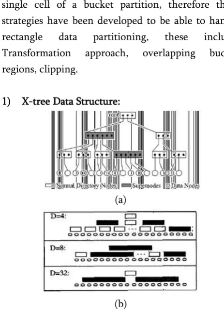
1) X-tree Data Structure:

(a)

(b)

Figure 2. (a) X-tree structure, (b) shapes of X-tree in different dimension of data [26].

regions but no strategy to avoid overlap. Each node there is of radius r, every node n and leaf node l residing in node N is at most distance r from N. the M-tree is balanced tree and does not requires periodical reorganization. On the other hand the X-tree prevents overlapping of bounding boxes which is a problem in high dimensionality. Any node that is not split will then result into super-nodes and in some extreme cases tree will linearize. The X-tree may be seen as a hybrid of a linear array-like and a hierarchical R-tree-like directory [26]. According to [16], the increase in the fan-out of the X-tree is the main positive side effect of the so called super-node strategy.

Advantage of the X-tree as given by [23]; [16] indicates that the X- tree is a heterogeneous access method because it is composed of nodes of different types. In most cases whereby it has become impossible to overcome or avoid overlap, super-nodes are created during the processes of inserting new entries into an X-tree. These super nodes accounts for the advantage of X-trees over all other access methods. Some of the benefits of the super-nodes include: a) Increase in average storage utilization due to fewer splits taking place and b) Reduction in height of tree due to increase in average tree fan-out. In cases where it is impossible to construct a hierarchical access method with minimized overlap between node bounding regions, then sequential scanning of the dataset is facilitated for very high-dimensional spaces. Further description of the structure of the X-tree according to [29]; as well as the “super-node”, the X-tree makes use of overlap-free algorithm and uses a the hierarchical directory structure for low dimensional vectors and a linear directory structure for high dimensional vector. These lead to fast access of the object attribute vector. However, the X-tree degrades on retrieval performance as dimensionality increases and brings about poor worst case performance than sequential scan when the number of dimensions is greater than 16, for low dimensionality, it means that

there is no overlap between the triangles. The X-tree applies the overlapping bucket regions which benefits from the possession of a key. Thus the Spatial object (or key) falls into a single bucket but the disadvantage here is that there are always multiple search paths due to the overlapping bucket regions. Nevertheless, the tree structure have been known to possess obvious limitations which include: (i) possibility of an overflow in the so called „super-nodes‟ (ii) unnecessary overhead induced by multiple disk access (iii) plus in some extreme cases the X- tree will totally linearize as such leads to inefficient memory management. This research work focuses on methods of building scalable large spatial database systems by extending the existing X-tree model to be able to overcome its limitations and therefore proposes a new heuristics based spatial indexing model; the adjusted X- tree ( aX-TREE) which is built upon the improvement of the existing models for efficient handling large data in a static environment. Many variations of the X-tree (X+-tree, VA-File, CBF e.t.c) has been proposed but none of these methods has shown total efficiency in large spatial data management.

2) X+-tree Data Structure:

VA-File and the CBF data structure:

The VA-File described in [29] was introduced to improve the retrieval performance deterioration of the X-tree, which falls into sequential scan in case of overgrown super-node in higher dimensional data. Using vector approximations (see fig.3), the number of disk I/O accesses is reduced and the high dimensional vector space is divided into sets of cells, which then generates an approximation of each cell to be able to scan the VA-File for a candidate cell when a user query is given. With this, the attribute vector within each candidate cells is searched to obtain its K-NN. The disadvantage of this method is that the algorithm may result to a conflicting query operation

Figure 3. the sample vector approximations [29].

III.

BULK LOADING TREE DATA STRUCTURE

Applying a bulk loading technique rather than the insertion operation of the existing X-tree will help to overcome the slower approach of individually inserting each object recursively and possible overcome the over expansion of the super-node. Once the data is sorted according to the any suitable ordering for spatial data, then a spatial data structure is then built on top of it and any n-dimensional data structure can be used for indexing the data, such as binary search trees and B-trees, R-trees X-trees e.t.c. [20]. In this way we may be able to overcome the challenge of un-expected overflow or overloading of the so called “super-node” that limits the efficacy of the existing X-tree. For static data, one of the best ways of building the data structure is by bulk-loading. Bulk-loading method builds a tree at a time instead of iteratively inserting each object into an initially empty tree one by one. A good bulk loading

method according to [31] would build fast for static objects and will ensure a lesser amount of

wasted empty spaces on the tree pages. [32] identified the advantages of the bulk loading a tree structure as the follows: 1. faster loading of the tree with all spatial objects at once 2. Reduced empty spaces in the nodes of the tree and 3. Better splitting of spatial objects into nodes of the tree.

A Data Sorting

particular, suppose we sort all of the cities in the US by their distance from Chicago, the process will be fine for finding the closest city to Chicago, say with population greater than 300,000. However, we cannot use the same ordering to find the closest city to New York, say with population greater than 300,000, without resorting the cities. The problem with two dimensions and higher according to [35] is that the notion of an ordering does not exist unless a dominance relation holds. This means that a point a = {ai |1 ≤ i ≤ d} is said to dominate a point b = {bi |1 ≤ i ≤ d} if ai ≤ bi, 1 ≤ i

≤ d. notwithstanding, using a space-filling curve according to [35]; [36], one can ensure the existence of an ordering by linearizing the data. Unfortunately such explicit ordering does not suit the requirements of having dynamically sorted the index structure when there is a change in query.

B Partitioning

[34] suggested few possible algorithms for packing a tree structure, which might help to split a node that is likely to overflow or already overflowing (although he limited the algorithms to r-tree packing only). These methods benefit the choice of partitioning strategy that has been adopted for decomposing the underlying space. Among these are:

1) Nearest-X method: [37] where objects are sorted by their first coordinate ("X") only and then split into pages of the desired size.

2) Sort-Tile-Recursive (STR): [33] another variation of Nearest- X, that estimates the total number of leaves required as⌈l = ⌉ number of objects/capacity of a node , the required split factor in each dimension to achieve this as p = l1/d , then repeatedly splits each dimensions successively into p equal sized partitions using 1-dimensional sorting for each split. The resulting pages, if they occupy more than one page, are again bulk-loaded using the same algorithm. For point data, the leaf nodes will not overlap, and

the data space would be "tiled" into approximately equal sized pages.

3) Packed Hilbert R-tree or the Hilbert Sort (HS) : [38] variation of Nearest-X, but sorting using the Hilbert value of the centre of a rectangle instead of using the X coordinate. There is no guarantee that the pages will not overlap

C Sort-tile Recursive Bulk-Loading

Sort-tile recursive –STR- method for sort - based (secondary sorting) bulk – loading proposed by [33] is a simple packing algorithm for efficient bulk-loading of data into a tree data structure, the algorithm has the potentials of improving the efficiency of the existing X-tree by loading the objects in bulk into memory, rather than the present direct insertion method. It will lead to an easy to implement polynomial-time algorithms and might most likely prove more efficient with larger data sets than the one used in the existing structure. Following the sort strategy, the aX-tree is built based on the sorted MBRs (rectangles) using a bottom – up rectangle packing approach. Some of the benefits of adopting this method is as follows for rectangle packing include:

 It‟s a typical example of a way of bulk-loading the existing X-tree

 It‟s a method commonly used in DBMS and GIS at the moment {32]

 Sort-Tile-Recursive has not been applied yet on the X-tree data structure

1. Simple to implement yet a has a good performance for query optimization

IV.

THE PROPOSED AX-TREE -INDEX

STRUCTURE

A Our Contributions

perspective. First, we argue that this is the first time that an adjusted X-tree based on secondary sorting is proposed for multidimensional data. Similar sort-based- algorithm might have been used in other

spatio-temporal data management indexing

structures (for instance the R-tree but not on the

X-tree). Most other methods for handling

dimensionality majors strictly on dimension reduction, feature based vector mapping, space reduction, feature embedding, point transformation etc. Also, previous work has based majorly on improving the R-tree and only a few amendments has been suggested for the improvement of the X-tree (which research has shown has a greater ability in terms of handling high dimensional spatio -temporal data as we have pointed out in section 2B 1)). Second, our system does not adopt the same similar insertion algorithm with existing X-tree, we differentiate our method by performing an initial secondary sort before packing the X-tree. The proposed aX-tree is expected to carry out the role of a filtering mechanism to reduce the costly direct examination of geometric objects induced by the increased overlap between the MBRs; thus, a systematic ordering of the intersecting hyper triangles in addition to reducing the extents of the MBRs may benefits query efficiency as fewer MBRs are expected to intersect. This is the goal the proposed aX-tree Index Structure is set to achieve.

B Motivation for aX-tree

[40], noted that current modelling research tends to focus on sampling and modelling techniques themselves and neglect studying and taking the advantages of characteristics of the underlying expensive functions. These always leave the problems of cost in high-dimensional data management and the problem of computational complexity un-tackled. For instance it is well established in the existing X-tree that in low dimensions the most efficient organization of the directory is a hierarchical organization which equates the height of the tree to the number of

required page accesses and it is also recognised, that for very high dimensionality a linear organization of the directory is more efficient. Then it suffices it to say that the X-tree is an inefficient data structure for high dimensional data management because while it is faster to access the linear part of the tree, without having to go through multiple paths, the X-tree still bear High implementation cost evolved from the overhead created by the super-node (especially in cases where a given query does not cover the entire MBR of the super node) and again it bears cost resulting from overhead induced by traversing the nodes of the hierarchical part of the tree. Moreover in some extreme cases the X-tree will totally linearizes as such leading to inefficient memory management. It has also been observed that in higher-dimensional data, many geometric data structures (including the X- tree – [26] and X+-tree which grows to further splitting of the super node and thereby degenerating to a clipped or disjoint region [30] fail to work well. Most of the existing variants of X-tree introduced to improve the X-tree are Cell/grid based. Cell/grid-based indexing approach needs point transformations to store spatial data and therefore does not provide a good spatial clustering. These disadvantages of the existing structure motivates a quest for a solution that overcomes them.

C Packing X-tree (aX-tree construction)

using one of two different approaches as descried in [41]; [42]: (1) by using the objects minimum bounding rectangles (MBRs – which is the smallest axis aligned rectangle enclosing a spatial object), enclosed with the points (xmin, xmax, Ymin, Ymax), so as to be able to estimate their extent in space using their minimum and maximum values for single measurements on each axis, and (2) by using a more accurate object decomposition technique where the spatial object (complex) is broken down into simple and smaller spatial component. If the first approach is adopted (which we did), then Afterwards, the tree construction follows steps described below. We

represent spatial object or query as

(xmin,ymin,xmax,ymax) in 2D space so points, lines and regions (or surfaces) can also be represented using MBRs.

D Algorithm description and Pre-processing

The algorithm starts with the pre-processing, which includes refining the table and converting the

LAT/LONG or X/Y coordinate column to standard geometric shape (points, polygons or lines) for spatial database, so as to get the extent.Following this phase, the algorithm then continues by building a bounding box (envelop) around the object‟s extent. The next phase consists of computing the midpoint of the bounding box, which is then sorted first by the X-coordinate of their centre point and then β (total nodes (page) required for the data) is computed as

explained later. R is the total database objects or rows and M is the maximum capacity of the node (explained later). In the next phase, the packing begins with the computation of (β1/d_{), where d stands}

for the dimension. This determines the total number of partitioning required for the data space. Based on the outcome of the partitioning, the rectangles are then loaded into pages in groups of M with rectangle ID, object ID and maximum node entry M as the input (i.e The algorithm take as input an array of pointers to a set rectangles and a description of maximum children count for each node). This phase returns the page/Node ID, and the MBR of the spatial

objects. We consider the centroids of the spatial objects rectangles (MBR) for ordering purpose because the simple heuristics behind aX-tree indexing is to first filter the nodes by the first coordinate ( e.g x-coordinate) and then filter the internal nodes on the subsequent coordinates (e.g y- and z- coordinates). After a successful partitioning, the entire dataset can then be scanned and each object is placed in the right partition based on the underlying interval (range). Fig.4 shows the general structure of the aX-tree in 2-dimension. To improve the space performance of the algorithm, the storage of data objects in aX-tree is such that the entry consist of the tree (3) important attribute (the object rectangle, rectangle id (ID), and the Maximum node entry (M)), which are the information necessary to differentiate between the data objects. This measure ensures a higher fan-out and a smaller directory (based on approximately 100% node fill), resulting in a better query performance and ensures that the area and perimeter of the resulting minimum bounding rectangles (MBRs) is minimized. Since the fan-out of the tree is determine by the page size (i.e. the size of the tree node that matches the page size) of the external memory, and because we have assumed that each tree node consume one disk page on the disk storage (as such, where M is the size of a disk page). Therefore, each non-leaf node will contain M

children or at least ≤ M/2. We compute the optimal value of the maximum node entry M to the tree as:

1.→ size of database (reduced by storing only the significant information)

2. → size of the block storage (page), typically 8kb for SQL sever

β→ total nodes (page) required for the data

tR → total rows or total number of database objects T → total nodes (Extent) required for the data

Wher

e ( )

) (

k b k b





 maximum node entry (m)

) 2 _______(



tR ceiling m

For example given a dataset with 0.500mb dataspace, 7313 data objects (rows), 8kb page size, the size of M

will be: 7313/ (0.500*1000KB/7.800KB) .

Alternatively, one could just in get the value of T as

Ω (in mb) * 128 (one extent in the block storage) for larger data and then get the value of M as tR/ T.

Intuitively, the calculation above guarantees a smaller directory than other indexes at all time for d

dimension.

Note for this experiment, the value of µ is applied as 8kb – (96 bytes + 36 bytes + 78bytes) = 7.800kb. The logic is simple: we subtracted 96bytes for the page header, 36bytes for row-offset and 78bytes free space on the page as typical of SQL server pages.

The idea of building the rectangles around the objects (by constructing the smallest enclosing block around them based on the value of the geometry or geography column of the database table) is adopted

to capture points and extended objects in a simple but efficient manner without having to create separate methods.

E Partitioning and Bulk-loading algorithm

Using the str algorithm, the partitioning is done logically through an interval (range) partitioning procedure. Spatially nearby objects are packed into one parent node. This guarantees that dead space in the parent MBR is minimized, and the parent MBR can be densely filled with child MBRs. The entire space is partitioned recursively until all the selected dimensions (x, y…N) are considered. Leaf node entry → (oId, MBR): oId is the tuple identifier for referring to an object in the database. MBR describes the smallest bounding n dimensional region around the data objects (for a 2d - space, the value of MBR will be of the form – xmin, xmax, ymin, ymax, and for 3d

space – xmin, xmax, ymin, ymax, zmin, zmax). Non-leaf node entry → (Cp, MBR, level): Cp is a (child) pointer to a lower level node and MBR is the rectangle enclosing it (which covers all regions in child node). PId identifies the partition (computing node) where the object is stored.

ALGORITHM 1: Partitioning

Input →(Obj ID, geometric col)

Build bounding box (bb) of objects as While R > 0

//Convert geometry column (geom) from table geom → Envelop (xmin, xmax, ymin, ymax) Compute Midpoint of bb

Midpoint → ([xmax – xmin], [ymax – ymin])/2 Sort rectangles (objects bounding box)

// Use value x-coordinate

Partition sorted rectangles into r → β 1/2 _{groups of vertical slices (partition)}

//β is explained later //for d >2, r → β 1/d

Sort r on the y – coordinate of the rectangles center. Repeat 1 to 5 for each selected dimension

Output → (MBR, Node ID), for each leaf level node that loaded into a temporary file to be processed in phase two of the aX-tree algorithm

Procedure two (2) begins with the temporary file that resulted from phase one. In this stage the new aX-tree is built recursively continuing upwards, until the root node is built starting from the leaves nodes.

ALGORITHM 2: Bulk-Loading

Create leaf nodes → the base level (L = 0)

While R /* in procedure 1*/ > 0 Create a new aX-tree node,

Allocate M rectangles (of R) to this node

/* during node creation avoid overlapping nodes, extend to super-node in the current level (only for leave level) see algorithm 3 */

Create nodes at higher level (L + 1) While (nodes at level L > 1)

Sort nodes at level L ≥0 on ascending creation time Repeat

Return Root

The simple heuristics in procedure 3, logically decides when it‟s appropriate to extend a node to super-node

ALGORITHM 3: Extend a Node (create super-node)

While creating the nodes in procedure 2

Do

Consider total number of MBRs in each partition Consider the value of M

For each partition

IF remaining RECTANGLE <= (M + ((M / 2) - 1))

&& RECTANGLE > M

&& RECTANGLE != 0

//RECTANGLE is used to represents objects that falls into individual partitions Create S (maximum number of entry for super-node)

{

S =M*2; M = S; }

END DO

Fig.4: the structure of the aX –tree in 2-dimension.

F Discussion and Experimental Analysis

construction in multidimensional data space when processing system and user queries. Therefore, Since overlap of bounding boxes is straight connect to query performance (because the access path of the query processing is effected directly by the overlap of directory nodes), which lead to multiple path and which according to [27] is the impending problem of the existing X-tree, and even the extension of the super- node unfortunately does not offer optimal solution for this problem in high dimensional data where overlap problem dominates the index eventually [43]. Hence, the main significance of our work is found in the unique technique for extending a node (to form a super node). From the discussions above, it is obvious that the ability to produce minimal, leave centred, non-overflowing super- node shields the structure from dearly deterioration. The proposed algorithm was implemented for 2D datasets; all our experiments were conducted using two-dimensional data for easy illustration. Nevertheless, the structure of algorithms can work for any number of dimensions. For illustrative purposes, we shall restrict our attention to 2-dimensional aX-trees with varying branching factor, depending on the application and resource at hand. It is important to remember that the nodes we refer to here relates to the pages on a disk (computer memory) therefore, building the tree structure should put into consideration the fact that minimum number of disk pages needs to be visited for any query operation for the indexing structure to be considered optimal.

1) Performance: The original X-tree, allows the size of a super-node to be many times larger than size of a normal node. In the X+-tree, the size of super-node is at most the size of a normal node multiplied by a given user parameter MAX_X_SNODE and when the super-node becomes larger than the upper limit, it is split into two new nodes. This two (2) scenarios have the tendency to deteriorate performance as such, we have limited the size of the super node to just a size double (2X) the normal node size and the formation (leave centric) is just a straightforward consideration of the value M for each partitions. In addition, to further improve this behavior, we have restricted the super node only at the leave level (as you can see in fig.4), as such, yielding an increased speed because increasing dimension but in our case, we are already guaranteed that the height only grows exponentially only at logM(R) – That is log in M base of R which

improves performance as the height of the tree is a function on M and M is optimized for space and speed efficiency.

Generally, the Performance of any tree search would be measured by the number of disk accesses (reads) necessary to find (or not find) the desired object(s) in the database. Therefore, the tree branching factor is chosen (as we have done) such that the size of a node is equal to (or a multiple of) the size of a disk block or file system page. In most database applications with high -dimensional data nearest neighbour queries are very important [26] therefore the main concern for nearest neighbour search (if the database was indexed with a tree data structure) is CPU-time rate which is always higher because the search is required to sort all the nodes based on their min-max distance. Fig.5(a), shows the performance of the proposed algorithm on a nearest neighbor query to find the nearest rectangle to a query point from a database of 81,177 polygon objects representing the different towns around our study area. fig.5(b) is the image of the packed rectangles.

it would not degenerate to a linear scan beyond the leave level as the super node is only created at the leave. In the second case, when there is no super node, the structure still promises a better performance as against the X-tree because it guarantees little or no overlap owing to the fact that the nodes contains equal objects which number is predetermined. Moreover, even when there are super nodes, they are quite few as such maintains overlap minimal partitioning. The only similar behavior between the two (2) structures is the height of the tree which behaves similar to that of the X-tree where the presence of increased number of super nodes forces the height of the tree to reduce. The super- node in this case is constructed such that after the partitioning, where objects are grouped according to the maximum node entries, I f the last group is less than the minimum allowed, then the last node in the partition is extended to super node. The justification for creating the super node in this manner, is to handle cases of highly skewed distributed data (which is very typical of spatial data), because unlike the case of uniformly distributed data where the MBRs are guaranteed to contains same amount of data, skewed datasets may vary by partition.

3): Basic operation: The algorithm has the functionalities for processing range queries, nearest neighbour queries point queries, join (intersection) queries and containment queries in a fast and efficient manner: fig (5a) shows the response time - 00:00:00.0000877μs - to a nearest neighbor query from a database of 81177 polygon objects.

Finally, another interesting thing about the proposed system is the ability to predict its performance based on disk page size. That is, great space efficiency is achieved by accurately predicting the space that would be consumed from the computation of total required pages. Moreso, a useful aspect of the

program is the fact that once the program executed and is running, increasing the table size (in any dimension) does not have any negative or overbearing effect on the program.

(a)

(b)

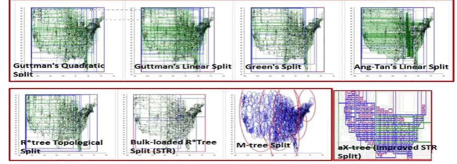
Figure 6. Comparison between our aX-tree algorithm and other splitting algorithms on a database with US postal districts

V.

Conclusion

We have discussed spatial indexing for managing large spatial database. The study reveals that the X-tree (designed for dynamic environment) has outstandingly performed well when it comes to indexing spatial data for efficient query performance. However, we discovered that the X- tree begins to in terms of space for large databases, thus this research examines the possibility of improving the X-tree and therefore proposes (aX-tree) a method of building a packed X-tree by bulk-loading the existing X-tree structure. The packed X-tree (aX -tree) outperforms the existing system in terms of speed and space management due to the mode of construction. It allows for the pre-processing of the data before loading into the structure. Bulk-loading method builds a tree at a time instead of iteratively inserting each object into an initially empty tree one by one. A good bulk loading method builds fast for static objects and will ensure a lesser amount of wasted empty spaces on the tree pages (by ensuring maximum node occupancy). The new aX-tree is performs faster by loading the tree with all spatial objects at once to reduce empty spaces in the nodes of the tree and thus producing a better splitting of spatial objects into nodes of the tree. Due to the leave centric super-node feature of the aX-tree, the structure benefits from: i) minimum tree height ii)

high directory node quality (being as hierarchical as possible) iii) minimum overlap and iv) reduced area the MBR and most importantly, maximized space efficency.

VI.

REFERENCES

[1]. Vieira, M. R. and Tsotras, V. J. (2013) Spatio-Temporal Databases: Complex Motion Pattern Queries. Springer

[2]. Tian, Y., Ji, Y., and Scholer, J. (2015) ―A prototype spatio-temporal database built on top of relational database‖. Paper presented at the 14-19. doi:10.1109/ITNG.2015.8

[3]. Samson, G. L., & Lu, J. (2016). PaX-DBSCAN: A PROPOSED ALGORITHM FOR IMPROVED CLUSTERING. In M. R. Pańkowska (Ed.) Studia Ekonomiczne. Zeszyty Naukowe, (269524th ed.). Katowice: Wydawnictwo Uniwersytetu Ekonomicznego w Katowicach. Retrieved from www.sbc.org.pl/Content/269524

[4]. Samson, G. L., LU, J., and XU, Q. (2016) Large spatial datasets: Present Challenges, future opportunities. Int'l Conference on Change, Innovation, Informaticsand Disruptive Technology,North America,dec.2016. Availableat:

<http://proceedings.sriweb.org/repository/index.p hp/ICCIIDT/icciidtt_london/paper/view/24>. Date accessed: 28 Dec. 2016.

Lu, & Q. Xu (Eds.), Ontologies and Big Data Considerations for Effective Intelligence (pp. 111-149). Hershey, PA: IGI Global. spatio-temporal database repairs‖. Paper presented at the 492-495. doi:10.1145/2525314.2525468

[7]. Kamlesh, K. Pandey., Rajat, K. Y., Anshu, D., and Pradeep, K. S. (2015), ―A Analysis of Different Type of Advance database System For Data Mining Based on Basic Factor‖, International Journal on Recent and Innovation Trends in Computing and Communication (IJRITCC), 3 (2) ISSN: 2321-8169, PP: 456 - 460, DOI: 10.17762/ijritcc2321-8169.150206 [8]. Billings, S. (2013) Nonlinear system

identification: NARMAX methods in the time, frequency, and spatio-temporal domains (1st ed.). Hoboken: Wiley.

[9]. Meng, X., Ding, Z., and Xu, J. (2014). Moving objects management: Models, techniques and applications (2; 2nd 2014; ed.). Dordrecht: Springer Berlin Heidelberg. doi:10.1007/978-3-642-38276-5

[10]. Huang, Y., and He, Z. (2015; 2014 ) ―Processing continuous K-nearest skyline query with uncertainty in spatio-temporal databases‖ Journal of Intelligent Information Systems, 45(2), 165-186. doi:10.1007/s10844-014-0344-1

[11]. Kang, C., Pugliese, A., Grant, J., & Subrahmanian, V. S. (2014). STUN: Querying spatio-temporal uncertain (social) networks. Social Network Analysis and Mining, 4(1), 1-19. doi:10.1007/s13278-014-0156-x

[12]. Moussalli, R., Absalyamov, I., Vieira, M. R., Najjar, W., and Tsotras, V. J. (2015; 2014;) ―High performance FPGA and GPU complex pattern matching over spatio-temporal streams‖. Geoinformatica, 19(2), 405-434. doi:10.1007/s10707-014-0217-3

[13]. Secchi, P., Vantini, S., and Vitelli, V. (2015) ―Analysis of spatio-temporal mobile phone data: A case study in the metropolitan area of milan‖ Statistical Methods & Applications, 24(2), 279-300. doi:10.1007/s10260-014-0294-

[14]. Eldawy, A., Mokbel, M. F., Alharthi, S., Alzaidy, A., Tarek, K., and Ghani, S. (2015) SHAHED: ―A MapReduce-based system for querying and visualizing spatio-temporal satellite data‖. Paper presented at the 1585-1596. doi:10.1109/ICDE.2015.7113427

[15]. Eldawy, A., & Mokbel, M. F. (2015, June). The Era of Big Spatial Data: Challenges and Opportunities. In 2015 16th IEEE International Conference on Mobile Data Management (Vol. Advance Tree Data Structures.arXiv preprint arXiv:1209.6495.

[18]. Ajit, S. and Deepak, G. (2011) "Implementation and Performance Analysis of Exponential Tree Sorting" International Journal of Computer Applications ISBN: 978-93-80752-86-3 24 (3) pp. 34-38.

[19]. Samet, H. (2009) ―Sorting spatial data by spatial occupancy‖ GeoSpatial Visual Analytics (pp. 31-43). Springer Netherlands.

[20]. Cazals, F., Emiris, I. Z., Chazal, F., Gärtner, B., Lammersen, C., Giesen, J., and Rote, G. (2013). ―D2. 1: Handling High-Dimensional Data‖. Computational Geometric Learning (CGL) Technical Report No.: CGL-TR-01.

[21]. Park, Y., Liu, L., and Yoo, J. (2013) ―fast and compact indexing technique for moving objects‖ Information Reuse and Integration (IRI), 2013 IEEE 14th International Conference on (pp. 562-569). IEEE.

[22]. Guting, R. H. (1994) ―An introduction to spatial database systems‖ The VLDB Journal—The International Journal on Very Large Data Bases, 3(4), 357-399.

[23]. Manolopoulos, Y., Nanopoulos, A., Papadopoulos, A. N., and Theodoridis, Y. (2010) R-trees: Theory and Applications. Springer Science and Business Media.

[24]. Jin, S., Kim, O., & Feng, W. (2013, June). MX-tree: a double hierarchical metric index with overlap reduction. In International Conference on Computational Science and Its Applications (pp. 574-589). Springer Berlin Heidelberg.

International Journal of Computer Science and Information Technologies. 6 (2) pp. 1737-1739. ISBN:0975-9646

[26]. Berchtold, S., Keim, D. A.., Kriegel, and Hans-Peter (1996). "The X-tree: An Index Structure for High-Dimensional Data". Proceedings of the 22nd VLDB Conference (Mumbai, India): 28– 39.

[27]. Berchtold, S., Keim, D. A., & Kriegel, H. P. (2001). An index structure for high-dimensional data. Readings in multimedia computing and networking. pp. 451.

[28]. Ciaccia, P., Patella, M., and Zezula, P., 1997. M-tree: An E cient Access Method for Similarity Search in Metric Spaces, in VLDB'97, pp. 426-435

[29]. Stuller, J., Pokorny, J., Bernhard, T. and Yoshifumi, M. (2000) Current Issues in Databases and Information Systems: East-European Conference on Advances in Databases and Information Systems Held Jointly with International Conference on Database Systems for Advanced Applications, ADBIS-DASFAA 2000 Prague, Czech Republic, September 5-9, 2000 Proceedings

[30]. Doja, M. N., Jain, S., and Alam, M. A. (2012) ―SAS: Implementation of scaled association rules on spatial multidimensional quantitative dataset‖ International Journal of Advanced Computer Science and Applications Vol. 3,(9) pp. 30-35 [31]. Mamoulis, N. (2012). Spatial data management

(1st ed.). Morgan & Claypool Publishers.

[32]. Giao, B. C., and Anh, D. T. (2015) ―Improving Sort-Tile-Recusive algorithm for R-tree packing in indexing time series‖ In Computing & Communication Technologies-Research, Innovation, and Vision for the Future (RIVF), 2015 IEEE RIVF International Conference on (pp. 117-122). IEEE.

[33]. Leutenegger, S. T., Edgington, J. M. and M. A. Lopez. (1997) "STR: A simple and efficient algorithm," in Proceedings 13th International Conference on Data Engineering, p. 497–506 [34]. Preparata F. P. and Shamos M. I. (1985.)

Computational Geometry: An Introduction. Springer-Verlag, New York.

[35]. Sagan H. (1994). Space-Filling Curves. Nueva York: Springer-Verlag.

[36]. Samet, H. (2006) Foundations of Multidimensional and Metric Data Structures: Mor-ganKaufmann

[37]. Roussopoulos, N., Kelley, S., & Vincent, F. (1995, June). Nearest neighbor queries. In ACM sigmod record (Vol. 24, No. 2, pp. 71-79). ACM. [38]. Kame I., and Faloutsos C. (1993) On Packing R-trees Proceedings of the second international conference on Information and knowledge management Pages 490-499.

[39]. Shan, S., and Wang, G. G. (2010) ―Survey of modeling and optimization strategies to solve high-dimensional design problems with computationally-expensive black-box functions‖ Structural and Multidisciplinary Optimization, 41(2), 219-241.

[40]. Lodi, A., Martello, S., and Monaci, M. (2002) "Two-dimensional packing problems: A survey". European Journal of Operational Research (Elsevier)141: 241–252. doi:10.1016/s0377-2217(02)00123-6.

[41]. Dolci, C., Salvini, D., Schrattner, M. and Weibel R. (2010) ―Spatial Partitioning and Indexing‖ Geographic Information Technology Training Alliance (GITTA). Available at: < International Conference on Database and Expert Systems Applications (pp. 207-223). Springer Berlin Heidelberg.

[43]. Assent I., Krieger R., Muller E. and Seidl T. (2007) DUSC: Dimensionality Unbiased Subspace Clustering IEEE International Conference on Data Mining (ICDM 2007), Omaha, Nebraska, USA, pages 409-414

[44]. Arya, S., Mount, D. M., Netanyahu, N.,