ISSN 2348 – 7968
Comparing Naive Bayes Method and Artificial Neural
Network for Semen Quality Categorization
Macmillan SimfukweP 1
P
, Douglas KundaP 1
P
and Christopher ChembeP 1
P
1
P
Center for ICT Education, Mulungushi University, Kabwe, P.O. Box 80415, Zambia
Abstract
One of the world wide health care concerns in the last two decades has been the decrease in fertility rates. The problem is said to be more severe among the male population. Research has shown that environmental factors and life style habits have an impact on the quality of semen. Orthodox diagnosis of seminal quality employs a laboratory approach, involving expensive tests, which are also sometimes uncomfortable to the patient. Application of machine learning techniques has been on the rise and has demonstrated encouraging results in many fields, including health care.
In this paper we propose Naïve Bayes and Artificial Neural Network classifiers for the characterization of seminal quality, based on environmental factors and life style habits Comparisons between the two classifier models show that their accuracy rate is the same and stands at 97%, on the training set.
Keywords: Artificial Neural Network, Naïve Bayes,
Semen Quality, Classification, Male Fertility
Potential
1. Introduction
The decline in male potential has been on the world wide health care concerns for the last two decades. Research has demonstrated that the main causes of this problem have been environmental and life style habits, such as smoking and alcohol consumption. Semen analysis is important for the evaluation of male fertility potential and can also be used for the assessment of sperm donors (Barrat et al, 1998).
In order to evaluate a male fertility potential, clinicians use the data obtained from semen analysis (Koletti, 2003) and compare the results with the corresponding reference value determined and set by the World Health Organization (WHO, 1999). Rowe and others (2000) recommend that the interpretation of results should be done by taking into consideration certain factors that may modify the semen parameters, such as fever, toxic exposure, childhood disease, etc.
Machine learning techniques have been applied in several fields, ranging from engineering disciplines to management and biomedical sciences. In the health care domain, expert and decision-support systems have been developed and used to improve efficiency. In our previous work, (Simfukwe et al, 2014), we suggested that the use of expert and decision-support systems may assist in addressing the shortage of medical personnel in developing countries. The benefits of using machine learning techniques in medical applications are further highlighted by Liboa and others (2006) and summarized as follows: (a) Easy optimization, leading to cost-effective and flexible non-linear modeling of large data sets; (b) good predictive accuracy, capable of supporting clinical decision making and (c) easier knowledge dissemination, with the provision of explanations on how decisions are arrived at.
The main objective of this paper is to compare Naïve Bayes and Artificial Neural Network models, as
applied to the problem of semen quality
categorization.
Naïve Bayesian classifier is a very attractive classifier has proved to be effective in many practical applications, including text classification, medical diagnosis, and systems performance management. Altheneyan et al (2014) applied the Naïve Bayes model for the author prediction of Arabic texts. The Naïve Bayes model has also been used for fault diagnosis in steam turbines (Wentao et al, 2014), Sales forecasting (Katkar et al, 2015 and automatic classification of webpages from a massive data network (LinBin et al, 2014).
Artificial neural networks have been widely applied for both classification and clustering problems. Ramzi and Zahari (2014) applied a back-propagation ANN for online recognition od? of handwritten Arabic characters, while Rajput and Verma (2014) proposed the utilization of a backpropagation feed forward ANN approach for speech recognition. ANN have also been used for feature reduction (Shah et al, 1999), in symmetric key cryptography (Sagar et al, 2015) and for leaf identification (Ankalaki et et, 2015).
We have used the male fertility data set from the UCI data set repository. The rest of the paper is arranged as follows: in section 2 we discuss our methodology, in section 3 we talk about our experiment's design, in section 4 we analyze and discuss the results. Finally, we draw some conclusions from our study and project some future research directions.
2. Methodology
2.1. Fertility Data set
The data set is obtained from the University of California Irvine (UCI) dataset repository. It consists of semen samples, obtained from 100 volunteers, and analyzed according to WHO 2010 criteria. The data set attributes are based on the fact that sperm concentration is affected by the social demographic and environmental factors, health status and life style habits. The data set can be summarized as follows:
• Number of Attributes: 9 plus the class attribute
• Number of instances: 100 • Missing attribute values: None
• Class distribution: There are 88 normal samples (88%) and 12 altered samples (12%)
Table 1 presents a description of the attributes and the range of their domain values.
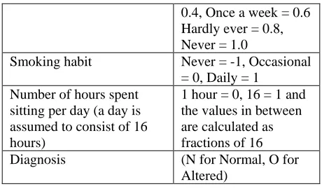
Table 1. Attribute description and domain value range
Attribute/Feature Domain Values
Season in which the
analysis was performed
Winter = 1, Spring = -0.33, Summer = -0.33, Fall = 1
Age at the time of analysis (18-36 range normalized to [0,1] range)
18-36 = 0, 36= 1 and the values in between are calculated as a fraction of 36 Suffered from childhood
diseases (e.g. chicken pox, mumps, measles, polio)
Yes = 0, No = 1
Suffered accident or serious trauma
Yes = 0, No = 1
Surgical intervention Yes = 0, No = 1 Suffered high fever in the
last year
Less than 3 months ago = -1, More than 3 months ago = 0, No = 1
Frequency of alcohol consumption
Several times a day = 0.0, Every day = 0.2 Several times a week =
0.4, Once a week = 0.6 Hardly ever = 0.8, Never = 1.0
Smoking habit Never = -1, Occasional = 0, Daily = 1 Number of hours spent
sitting per day (a day is assumed to consist of 16 hours)
1 hour = 0, 16 = 1 and the values in between are calculated as fractions of 16 Diagnosis (N for Normal, O for
Altered)
The data collection and preprocessing (normalization) procedure for this data set is described in Gil et al (2012).
2.2. Naïve Bayes
Naïve Bayes (NB) is a simple technique for constructing classifiers: models that assign class labels to problem instances, represented as vectors of feature values, where the class labels are drawn from some finite set. Naive Bayes classifiers are based on the assumption that the features are independent of each other, given the class variable. Now let us derive a Naïve Bayes model for our problem (fertility dataset).
Let 𝑆= {𝑓𝑓1,𝑓𝑓2, … … .𝑓𝑓𝑛} be a set of the features, such as those presented in table 1, where n denotes the total number of features, respectively. Let each instance 𝑋𝑗𝑗𝜖�𝑋1,𝑋2, … …𝑋𝑝𝑝�=𝑃, where p is the total number of instances, be represented by the same feature set S. Let 𝐶𝑖𝜖{𝐶1,𝐶2, … …𝐶𝑚} =𝐶 be a class to which a particular instance, 𝑋𝑗𝑗, belongs depending on the values of its features. The Naïve Bayes Learner is to categorize/classify an instance, 𝑋𝑗𝑗, based on the assumption that the elements of set S
(features) assume their values independent on one another. The Naïve Bayes classifier attributes a new instance, expressed in the form of feature set S, to the most probable target class 𝐶𝑖 according to equation 1.
𝐶𝑖=𝑎𝑎𝑟𝑔𝑚𝑎𝑎𝑥𝑥𝐶𝑖𝜖𝐶𝑃(𝐶𝑖|𝑓𝑓1,𝑓𝑓2, … … …𝑓𝑓𝑛) (1)
The probability 𝑃(𝐶𝑖|𝑓𝑓1,𝑓𝑓2, … … …𝑓𝑓𝑛) must be calculated for each 𝐶𝑖𝜖𝐶 using the following Bayes formula:
𝑃(𝐶𝑖|𝑓𝑓1,𝑓𝑓2, … …𝑓𝑓𝑛) =
𝑃(𝑓𝑓1,𝑓𝑓2, … … ,𝑓𝑓𝑛|𝐶𝑖) ×𝑃(𝐶𝑖)⁄𝑃(𝑓𝑓1,𝑓𝑓2, … … ,𝑓𝑓𝑛) (2)
where 𝑃(𝑓𝑓1,𝑓𝑓2, … … ,𝑓𝑓𝑛)≠0.
ISSN 2348 – 7968 Assuming the uniformity of {𝑓𝑓1,𝑓𝑓2, … … .𝑓𝑓𝑛}, equation
2 can be simplified into equation 3.
𝑃(𝐶𝑖|𝑓𝑓1,𝑓𝑓2, … …𝑓𝑓𝑛) =𝑃(𝑓𝑓1,𝑓𝑓2, … …𝑓𝑓𝑛|𝐶𝑖) ×𝑃(𝐶𝑖) (3)
Applying the chain rule, we get:
𝑃(𝑓𝑓1,𝑓𝑓2, … …𝑓𝑓𝑛|𝐶𝑖) ×𝑃(𝐶𝑖) =
𝑃(𝐶𝑖) ×∏𝑛𝑘=1𝑃(𝑓𝑓𝑘|𝐶𝑖) (4)
Therefore the quality of semen sample is categorized to a particular class 𝐶𝑖 , according to equation 5.
𝐶𝑖=𝑎𝑎𝑟𝑔𝑚𝑎𝑎𝑥𝑥𝐶𝑖𝜖𝐶𝑃(𝐶𝑖)∏𝑛𝑘=1𝑃(𝑓𝑓𝑘|𝐶𝑖) (5)
Where the probability P(𝐶𝑖) is estimated by the frequency of instances belonging to class 𝐶𝑖in the training data set.
𝑃(𝐶𝑖) =𝑡𝑜𝑡𝑎𝑙𝑛𝑢𝑚𝑏𝑒𝑟𝑛𝑢𝑚𝑏𝑒𝑟𝑜𝑓𝑜𝑓𝑖𝑛𝑠𝑡𝑎𝑛𝑐𝑒𝑠𝑖𝑛𝑠𝑡𝑎𝑛𝑐𝑒𝑠𝑏𝑒𝑙𝑜𝑛𝑔𝑖𝑛𝑔𝑖𝑛𝑡ℎ𝑒𝑡𝑟𝑎𝑖𝑛𝑖𝑛𝑔𝑡𝑜𝑐𝑙𝑎𝑠𝑠𝑑𝑎𝑡𝑎𝐶𝑖 𝑠𝑒𝑡 (6)
𝑃(𝑓𝑓𝑘|𝐶𝑖) can be estimated using a Gaussian
distribution (Altheneyan et al, 2014), using equation 7:
𝑃(𝑓𝑓𝑘|𝐶𝑖) =𝑔(𝑓𝑓𝑘,𝜇𝑘,𝜎𝑘)
𝑔(𝑓𝑓𝑘,𝜇𝑘,𝜎𝑘) =√2𝜋𝜎1 𝑘𝑒
(𝑓𝑘−𝜇𝑘)2
2𝜎𝑘2 , (𝜎> 0) (7)
2.3. Artificial Neural Network
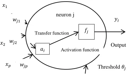
An artificial neural network (ANN) consists of a pool of simple processing units, called neurons, which communicate by sending signals to each other over a large number of weighted connections (Krose and Van der Smagt, 1996). The neurons are grouped together to from layers, thus an ANN consists of: (1) the input layer which receives inputs from the external environment, the hidden layer(s) (optional), and the output layer which generates the results (e.g. classification results). Figure 1 presents a feed forward ANN, with one hidden layer. Except for the input layer neurons, every neuron is a computational element with an activation function. The principle mechanism of the ANN is that when data is presented to the input layer, the network neurons run computations in the subsequent layers until an output value is yielded at each of the neurons in the output layer.
Figure 1. Multi-layer feed forward ANN
Each neuron in a particular, except for the output layer neurons, feeds its output as input for the neurons in the next layer. The neurons in the processing layers (i.e. hidden and output layers) computes weighted sums of their inputs and add a threshold. The resulting sums are then used to compute the activation levels of the neurons by applying an activation function (e.g. sigmoid function). The process can be defined as follows.
𝑎𝑎𝑗𝑗=∑𝑝𝑝𝑖=1𝑤𝑤𝑗𝑗𝑖𝑥𝑥𝑖+𝜃𝜃𝑗𝑗 , 𝑦𝑦𝑗𝑗=𝑓𝑓𝑗𝑗(𝑎𝑎𝑗𝑗) (8)
where 𝑎𝑎𝑗𝑗 is the activation of neuron j, which is equal to the sum of the weighted sum of the inputs
𝑥𝑥1,𝑥𝑥2, … … . ,𝑥𝑥𝑝𝑝 and the threshold 𝜃𝜃𝑗𝑗, 𝑤𝑤𝑗𝑗𝑖 is the connection weight from neuron i to neuron j, 𝑓𝑓𝑗𝑗 is the activation function for the 𝑗𝑡ℎ neuron and 𝑦𝑦𝑗𝑗 is the output. Figure 2 shows a graphical representation of how a neuron processes information.
Figure 2. A processing neuron
The sigmoid function is popularly used as the activation function and is defined as:
𝑎𝑎𝑗𝑗
𝑓𝑓𝑗𝑗
Transfer function
Activation function
neuron j
𝑦𝑦𝑗𝑗
Output
Threshold 𝜃𝜃𝑗𝑗
𝑥𝑥1
𝑤𝑤𝑗𝑗1
𝑥𝑥2 𝑤𝑤𝑗𝑗2
𝑥𝑥𝑝𝑝 𝑤𝑤𝑗𝑗𝑝𝑝
𝑓𝑓(𝑡) = 1+𝑒1−𝑡 (9)
A single neuron in a multi-layer ANN is able to linearly separate the input space into subspaces by means of a hyper plane defined by the weights and the threshold, where the weights define the direction of the hyper plane and the threshold offsets it from the origin (Gil et al, 2012).
In order to train a multi-layer feed forward ANN, we employ supervised learning based on the
backpropagation algorithm (Rumelhart, Hinton and Williams, 1986). The backpropagation algorithm is a gradient descent method for the adaptation of connection weights. Here is how the backpropagation algorithm works:
All the weight vectors 𝑤𝑤𝑖 are initialized with small random values from a pseudorandom sequence generator. Then and until the convergence (i.e. when the error E is below a preset value) we repeat the three basic steps:
1. The weight vectors 𝑤𝑤𝑖 are updated by
𝑤𝑤(𝑡+ 1) =𝑤𝑤(𝑡) +𝛥𝑤𝑤(𝑡) (10)
2. Where
𝛥𝑤𝑤(𝑡) =−𝛼𝜕𝐸(𝑡)/𝜕𝑤𝑤 (11) 3. Compute the error E(t+1), where t is the
iteration number, w is the weight vector and
𝛼 is the learning rate. The backpropagation algorithm adapts the weights and the thresholds of the neurons in a way that minimizes the error function:
𝐸=12∑𝑛𝑝𝑝=1(𝑑𝑝𝑝− 𝑦𝑦𝑝𝑝)2 (12)
where 𝑦𝑦𝑝𝑝 is the actual output and 𝑑𝑝𝑝 is the desired output for input pattern/instance p.
The minimization of E can be accomplished by gradient descent, i.e. the weights are adjusted to change the value of E in the direction of its negative gradient. The exact updating rules can be computed by applying the derivatives and the chain rule.
3. Experiment Design
The experiments were conducted in the Mat Lab R2014a platform on computer equipped with 1.00 GHZ processor and 4GB RAM.
The dataset was first imported into Mat Lab with the help of the Mat Lab import wizard, and saved in the form of two matrices; a 100 by 9 matrix for the
attribute values and a 100 by 1 for the class labels (for the NB model) or a 100 by 2 (for the ANN model).
3.1. Building and training of the Naïve Bayes Classifier
The Naïve Bayes model was created and trained using the "fitNaiveBayes" command contained in Mat Lab, and figure 3 presents the results of invoking this command.
Figure 3. Creating the Naïve Bayes classifier
Value indicates the class label. In this case, 0 is for normal and 1 is for altered. Count shows the
distribution or number of samples in each class, while percent shows the number of samples in each class as a percentage of the total number of samples in the data set.
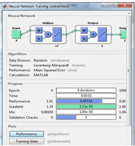
3.2. Building and training of the Neural Network Classifier
The ANN model was created using a set of Mat Lab built-in commands. Figure 4 presents a graphical summary of the creation and training process for the ANN model.
ISSN 2348 – 7968
Figure 4. Creating and building the ANN classifier
An ANN with 9 neurons in the input layer (since we have nine attributes), 17 neurons in the hidden layer (determined experimentally) and 2 neurons in the output layer (since we have 2 possible outputs), was created. For training we used the Levenberg-Marquardt training approach and the Mea Squared Error for performance assessment. The data set is partitioned as follows: 70% of the samples are used for training, 15% for validation and 15% for testing.
3.3. Testing the Classifiers and Results Analysis
Validation of the classifiers is done using the training data samples, and the validation results are presented in the form of confusion matrices, shown in tables 2 and 3.
Table 2. Confusion matrix for ANN on training data samples
Positive Negative
Positive 86 (TP) 1 (FN)
Negative 2(FP) 11 (TN)
Table 3. Confusion matrix for NB on training data samples
Positive Negative
Positive 86 (TP) 2 (FN)
Negative 1 (FP) 11 (TN)
We can compute the accuracy rates for the two classifiers suing equation 13.
𝐴𝑐𝑐𝑢𝑟𝑎𝑐𝑦𝑟𝑎𝑡𝑒=𝑇𝑃+𝑇𝑁+𝐹𝑁+𝐹𝑃𝑇𝑃+𝑇𝑁 × 100 (13)
Where TP, TN, FN and FP stand for true positive, true negative, false negative and false positive, respectively.
The accuracy rates for both classifiers on the training dataset are equal and stand at 97%. However, this does not guarantee good performance on unseen data samples.
The two classifiers were further tested on randomly generated unseen data samples, presented in table 4. F1 through to F9 are the attributes columns, presented in table 1, and in the class column, N stands for "normal" and O stands for "altered".
Table 4. Randomly generated unseen data samples
F1 F2 F
3 F 4
F 5
F 6
F7 F
8
F9 Clas
s 1
-0.3 3
0.6 9
0 1 1 0 0.
8
0 0.8 N
2 -0.3 3
0.9 4
1 0 1 0 0.
8
1 0.3
1 O
3 1 0.6
4
0 0 1 0 0.
8
-1 0.2 5
N
4 1 0.6
9
1 0 1 0 0.
8
-1 0.2 5
O
5 -0.3 3
0.5 1 1 0 -1 0.
8
0 0.8
8 O
The results were as follows: the accuracy rate for the NB classifier was 80%, while that of the ANN classifier was also 80%. Tables 5 and 6 present the test results on unseen data samples.
Table 5. Confusion matrix for ANN on unseen data samples
Positive Negative
Positive 2 (TP) 1 (FN)
Negative 0(FP) 2 (TN)
Table 6. Confusion matrix for NB on unseen data samples
Positive Negative
Positive 1 (TP) 1 (FN)
Negative 0 (FP) 3 (TN)
4. Conclusions
We have experimented with two popular machine learning techniques to classify the quality of human semen, in order to assess the male fertility potential. Our dataset is highly imbalanced and biased towards the "Normal" class (88%) and this has an impact on the accuracy rate (80%) of the classifiers, on unseen data samples. We can develop a decision support system for the assessment of male fertility potential, based on the techniques. Such a system can be used for preliminary assessment of semen quality before more elaborate, expensive and uncomfortable tests are conducted on the patient.
In future we would strive to improve the classification accuracy on unseen data samples by employing classifier fusion. This is to ensure that different classifiers complement each other, since they use different assumptions as regards the data; they are likely to make different mistakes. This fact is evident from the results presented in tables 5 and 6; i.e. even though both classifiers have the same accuracy, their true positive (TN) and true negative (TN) results are different, for the same unseen data samples. We would also like to experiment with other machine learning techniques on this data set and compare the results.
References
[1] Barrat C.L., Clements S., Kessopoulou E. (1998). Semen Characteristics and fertility tests required for storage of spermatozoa. Human Reproduction (Oxford, England), 13(Suppl. 2). 1-7. Discussion 8-11
[2] Koletti P.N. (2003). Evaluation of the subfertile man. American Family Physician, 67 (10), 2165-2172
[3] WHO (1999). WHO laboratory manual for the examination of human semen and sperm-cervical mucus interaction (4th ed.). Published on behalf of the World Health Organization by Cambridge University Press, Cambridge, UK
[4] Rowe P.J., Comhaire F.H. (2000). WHO manual for the standardized investigation, diagnosis and management of the infertile male, Cambridge University Press
[5] Lisboa P.J, Taktak A.F.G. (2006). The use of artificial neural networks in decision support in cancer: A systematic review. Neural Networks, 19(4), 408-425
[6] Simfukwe M, Kunda D, Zulu M. (2014). Addressing the shortage of medical doctors in Zambia: Medical diagnosis expert system as a solution. IJISET, Vol. 1 Issue 5
[7] David Gil, Jose Luis Girela, Joaquin De Juan, M. Jose Gomez-Torres, and Magnus Johnsson. Predicting seminal quality with artificial intelligence methods. Expert Systems with Applications, 39(16):12564 – 12573, 2012
[8] Altheneyan A.S., Menai M.B.. Naïve Bayes classifiers for authorship attribution of Arabic texts. Journal of King Saudi University – Computer and Information Sciences (2014) 26, 473-484
[9] Huang Wentao; Yu Jun; Zhao Xuezeng; Lu Xiaojun. Fault diagnosis for steam turbine based on flow graphs and naïve Bayesian classifier. Mechatronics and Automation (ICMA), IEEE International Conference 2014
[10] Xu LinBin; Liu Jun; Zhou WenLi; Yan Qing. Adaptive Naive Bayesian Classifier for Automatic Classification of Webpage from Massive Network Data. Intelligent Human-Machine Systems and Cybernetics (IHMSC), Sixth International Conference on 2014
[11] Katkar, V.; Gangopadhyay, S.P.; Rathod, S.; Shetty, A. Sales forecasting using data warehouse and Naïve Bayesian classifier. Pervasive Computing (ICPC), International 2015
[12] Xu LinBin; Liu Jun; Zhou WenLi; Yan Qing. Adaptive Naive Bayesian Classifier for Automatic Classification of Webpage from Massive Network Data. Intelligent Human-Machine Systems and Cybernetics (IHMSC), Sixth International Conference on 2014
[12] Krose B., Van der Smagt P., An Introduction Neural Networks. University of Armsterdam, 8th Edition, 1996 [13] Rumelhart D.E., Hinton G.E., Williams R.J, Learning representations by backpropagating errors. Nature, 323, 533-536. 1986
[14] Ramzi, A.; Zahary, A. Online Arabic handwritten character recognition using online-offline feature extraction and back-propagation neural network. Advanced Technologies for Signal and Image Processing (ATSIP), 1st International Conference 2014
[15] Rajput, N.; Verma, S.K. Back propagation feed forward neural network approach for Speech Recognition. Reliability, Infocom Technologies and Optimization (ICRITO) (Trends and Future Directions), 3rd International Conference 2014
[16] Shah, B.; Trivedi, B.H. Reducing Features of KDD CUP 1999 Dataset for Anomaly Detection Using Back Propagation Neural Network. Advanced Computing & Communication Technologies (ACCT), Fifth International Conference 2015
[17] Sagar, V.; Kumar, K. A symmetric key cryptography using genetic algorithm and error back propagation neural network. Computing for Sustainable Global Development (INDIACom), 2nd International Conference 2015
ISSN 2348 – 7968
[18] Ankalaki, S.; Majumdar, J. Leaf identification based on back propagation neural network and support vector machine. Cognitive Computing and Information Processing (CCIP), International Conference 2015
Macmillan Simfukwe is currently pursuing a PHD in Computer
Science at Southwest Jiaotong University in China. He holds a Bachelor of Applied Informatics Degree and a Master of Applied Informatics Degree, both obtained from the St. Petersburg State University of Engineering and Economics in Russia. He is also a Lecturer at Mulungushi University in the Center for ICT Education in Zambia. . He is doing is PHD research under the Key Lab of Cloud Computing and Intelligent Technology of Sichuan Province, china. He is also a member of the computer society of Zambia. His research areas of interest include machine learning, data mining, computer vision, health informatics and enterprise information systems
Dr Douglas Kunda holds a Doctorate Degree from the University
of York, UK. He is currently the Director of the Center for ICT Education at Mulungushi University in Zambia. He is a fellow of the Computer Society of Zambia and a member of the Association of Computing Machinery. He worked as project manager for the Integrated Financial management Information System (IFMIS) project for the Ministry of Finance of Zambia and he is a certified SAP ERP Solution Manager Consultant.
Christopher Chembe is currently pursuing a PHD in Computer
Science at the University of Malaya in Malaysia. He holds a BSc in Computer Science from University of Zambia and a Master's Degree in Computer from University of Malaysia. He is also a lecturer at Mulungushi University, Zambia, in the Center for ICT Education. He is a member of the Computer Society of Zambia. His areas of research wireless networks, ad hoc networks and internet of vehicles.