Investigating temporal field sampling strategies for site specific calibration of three soil moisture–neutron intensity parameterisation methods

www.hydrol-earth-syst-sci.net/19/3203/2015/ doi:10.5194/hess-19-3203-2015

© Author(s) 2015. CC Attribution 3.0 License.

Investigating temporal field sampling strategies for site-specific

calibration of three soil moisture–neutron intensity

parameterisation methods

J. Iwema1, R. Rosolem1,2, R. Baatz3, T. Wagener1,2, and H. R. Bogena3

1_{Department of Civil Engineering, University of Bristol, Queen’s Building, Bristol, UK} 2_{Cabot Institute, University of Bristol, Bristol, UK}

3_{Agrosphere (IBG-3), Forschungszentrum Jülich GmbH, 52425 Jülich, Germany} Correspondence to: J. Iwema ([email protected])

Received: 29 January 2015 – Published in Hydrol. Earth Syst. Sci. Discuss.: 24 February 2015 Revised: 18 June 2015 – Accepted: 9 July 2015 – Published: 24 July 2015

Abstract. The Cosmic-Ray Neutron Sensor (CRNS) can provide soil moisture information at scales relevant to hy-drometeorological modelling applications. Site-specific cali-bration is needed to translate CRNS neutron intensities into sensor footprint average soil moisture contents. We investi-gated temporal sampling strategies for calibration of three CRNS parameterisations (modifiedN0, HMF, and COSMIC) by assessing the effects of the number of sampling days and soil wetness conditions on the performance of the calibration results while investigating actual neutron intensity measure-ments, for three sites with distinct climate and land use: a semi-arid site, a temperate grassland, and a temperate for-est. When calibrated with 1 year of data, both COSMIC and the modified N0 method performed better than HMF. The performance of COSMIC was remarkably good at the semi-arid site in the USA, while theN0modperformed best at the two temperate sites in Germany. The successful performance of COSMIC at all three sites can be attributed to the bene-fits of explicitly resolving individual soil layers (which is not accounted for in the other two parameterisations). To better calibrate these parameterisations, we recommend in situ soil sampled to be collected on more than a single day. However, little improvement is observed for sampling on more than 6 days. At the semi-arid site, the N0mod method was cali-brated better under site-specific average wetness conditions, whereas HMF and COSMIC were calibrated better under drier conditions. Average soil wetness condition gave better calibration results at the two humid sites. The calibration re-sults for the HMF method were better when calibrated with

combinations of days with similar soil wetness conditions, opposed toN0modand COSMIC, which profited from using days with distinct wetness conditions. Errors in actual neu-tron intensities were translated to average errors specifically to each site. At the semi-arid site, these errors were below the typical measurement uncertainties from in situ point-scale sensors and satellite remote sensing products. Nevertheless, at the two humid sites, reduction in uncertainty with increas-ing samplincreas-ing days only reached typical errors associated with satellite remote sensing products. The outcomes of this study can be used by researchers as a CRNS calibration strategy guideline.

1 Introduction

(Wood et al., 2011; Robinson et al., 2008; Vereecken et al., 2008).

A recent technology that may help fill this scale gap, is the Cosmic-Ray Neutron Sensor (CRNS) (Zreda et al., 2008, 2012). The CRNS detects fast neutrons, which are produced from high-energy neutrons of cosmic origin and are further attenuated as they travel through the soil (Hess et al., 1961; Zreda et al., 2008). Because of the high attenuation power of hydrogen for these cosmic-ray neutrons, fast neutron inten-sity decreases with increasing hydrogen content within the sensor footprint (Zreda et al., 2008). Through this inverse relationship with hydrogen content, fast neutron intensity is non-linearly related with soil moisture content (Zreda et al., 2008). The sensor footprint has a horizontal effective area of about 600 m diameter at sea level for dry air but changes slightly with elevation and soil moisture content in the atmo-sphere (Desilets and Zreda, 2013). The measurement depth varies between about 12 (wet conditions) and 76 cm (dry con-ditions) (Zreda et al., 2008).

Site-specific neutron intensity–soil moisture relationships should be determined to derive soil moisture values, i.e. the CRNS needs site-specific calibration. The fully empiricalN0 formula (Desilets et al., 2010) is usually deployed for this calibration (Zreda et al., 2012). However, not only soil mois-ture content affects the fast neutron intensity (Franz et al., 2013c). All other hydrogen pools, (e.g. biomass, snow) af-fect the signal, complicating the finding of a unique rela-tionship between neutron intensity and soil moisture con-tent for a variety of sites and conditions (Zreda et al., 2012). Therefore a universal calibration function, the hydrogen mo-lar fraction method (HMF), was developed, which assumes a relationship between hydrogen prevalence and neutron in-tensity (Franz et al., 2013b). WhileN0and HMF both calcu-late an integrated, depth-weighted profile average soil mois-ture content, the COsmic-ray Soil Moismois-ture Interaction Code (COSMIC) computes neutron intensities from soil moisture profiles (Shuttleworth et al., 2013) and can be directly ap-plied in the context of hydrometeorological data assimilation (Rosolem et al., 2014).

Typically only a single parameter (N0) of theN0-method needs to be calibrated with a single point from average soil moisture, representative of the CRNS footprint (Desilets et al., 2010; Zreda et al., 2012). A similar approach is typ-ically used for HMF, although estimates of additional hy-drogen pools are also needed (Franz et al., 2013b). Orig-inally, COSMIC was site-calibrated against neutron parti-cle transport model Monte Carlo N-Partiparti-cle eXtended (MC-NPX, Pelowitz, 2005), using 22 hypothetical profiles cover-ing a range of possible soil moisture profiles, but weighted towards the more probable profiles at each considered site (Shuttleworth et al., 2013).

Although a number of investigations have used single cal-ibration points from measured soil moisture profiles for each of the three methods (Rivera Villarreyes et al., 2011; Zreda et al., 2012; Franz et al., 2013c; Bogena et al., 2013; Baatz

et al., 2014), to our record, there has been no previous study on whether this is feasible for each of these three methods at distinct sites. The fact that hydrogen pools (e.g. biomass, litter layer water) vary differently over time than soil mois-ture content profiles, and that not all these hydrogen pools can always be monitored completely and accurately (Bogena et al., 2013; Rivera Villarreyes et al., 2011), could be a com-plicating factor. Therefore we posed the following research questions:

– What are the benefits and limitations of the three dif-ferent soil moisture–neutron intensity parameterisation methods (N0, HMF and COSMIC) across sites with dis-tinct climates and land cover types?

– How often should soil moisture profiles be sampled in order to reliably calibrate the three soil moisture– neutron intensity parameterisation methods?

– Under what type of wetness conditions or combina-tions of wetness condicombina-tions should soil moisture profiles be sampled in order to reliably calibrate the three soil moisture–neutron intensity parameterisation methods? In order to answer these questions, we calibrated the three parameterisation methods for three sites with distinct types of land cover and climate: a semi-arid, sparsely vegetated site, a humid grassland, and a humid spruce forest. We used data from 2012 to evaluate whether different days or differ-ent combinations of days would lead to differdiffer-ent calibration results and to investigate our hypothesis that a single cali-bration day is not always sufficient. We used depth-weighted average soil moisture content to see whether wetness condi-tions affect calibration results, and whether combinacondi-tions of days with different wetness conditions would yield different calibration results.

2 Materials and methods 2.1 Methodology

Table 1. Temporal sampling strategies and their theoretical numbers

of combinations.

Strategy Number of days Theoretical number of from data series combinations for

Santa Rita Creosote (SR)

1DAY any 1 day 362 2DAY any combination of 2 days 6.5×104 4DAY any combination of 4 days 7.0×108 6DAY any combination of 6 days 3.0×1012 10DAY any combination of 10 days 9.4×1018 16DAY any combination of 16 days 3.0×1027

combined use of CRNS and sensor networks has been essen-tial for understanding and improving this technology (Franz et al., 2013b; Rosolem et al., 2014; Bogena et al., 2013; Baatz et al., 2014). Despite having slightly different uncertainties compared to gravimetric/volumetric soil samples obtained in the field, in situ sensors have been already successfully used in previous studies for comparison of CRNS and smaller-scale soil moisture sensors (Franz et al., 2012; Bogena et al., 2013; Baatz et al., 2014).

2.2 Site and data description 2.2.1 Santa Rita Creosote (SR)

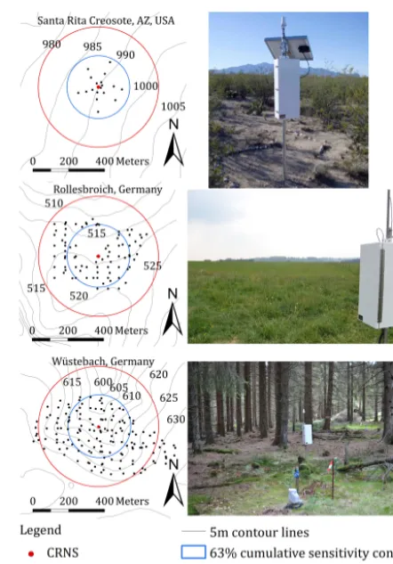
Santa Rita Creosote (Table 2 and Fig. 1), hereinafter referred to as SR, is a semi-arid site in Arizona, USA (Scott et al., 1990), which is sparsely vegetated (∼24 % of surface area) with creosote bush (∼14 % of surface area) and other species of bushes, grasses, and cacti (Cavanaugh et al., 2011). Day-time temperatures above 35◦C in summer and above 15◦C in winter are common, and precipitation falls mostly in sum-mer and winter (Scott et al., 1990; Franz et al., 2012). The soil texture can be characterised as sandy loam with 5 to 15 % gravel (Cavanaugh et al., 2011). At SR 18 paired in situ sensor profiles, with sensors (ACC-SEN-TDT, Acclima Inc., Meridian,ID,USA) at 5, 10, 20, 30, 50, and 70 cm depth, were installed with the spatial distribution as described by Franz et al. (2012), with all equal horizontal weights (less than 1 % of missing data). We computed a simple mean hor-izontal soil moisture content for each sensor layer on every day.

2.2.2 Rollesbroich (RB)

Rollesbroich (Table 2 and Fig. 1), located in Germany and hereinafter referred to as RB, is a humid grassland site, dom-inated by rye grass and smooth meadow grass (Baatz et al., 2014). The seasonality in precipitation is small, with on av-erage 540 mm in winter and 610 mm in summer (DWD, 2014). Average temperatures are 4.9◦C in winter and 10.9◦C in summer (DWD, 2014). The soil contains mainly silt (∼ 61 %) and some sand (∼20 %) and clay (∼18 %) (Qu et al.,

Figure 1. Maps and photos of the three research sites; Santa Rita

Creosote (SR), Rollesbroich (RB), and Wüstebach (WB). The cu-mulative uncertainty contours indicate the relative areal contribu-tions to the CRNS-signal. The 86 % contour represents the theoret-ical CRNS footprint (Zreda et al., 2008).

2014). The in situ sensor network (SoilNet, Qu et al., 2013, 2014) consisted of 83 profiles with soil moisture sensors (SPADE soil water content probes, sceme.de GmbH i.G., Horn-Bad Meinberg, Germany; Hübner et al., 2009) installed at 5, 20, and 50 cm depth (with ∼15 % of missing data). While the sensor profiles at SR were positioned such that all had equal weights, this was not the case at RB, where we calculated horizontal average daily soil moisture contents by assigning weights to the sensor profiles representing their distance to the CRS, as described in Bogena et al. (2013). 2.2.3 Wüstebach (WB)

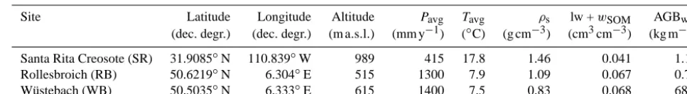
Table 2. Characteristics of the three study sites. Information for SR is from Shuttleworth et al. (2013); Franz et al. (2013b); Scott et al.

(1990); Cavanaugh et al. (2011); WRCC (2006). Information for RB and WB is from Baatz et al. (2014).

Site Latitude Longitude Altitude Pavg Tavg ρs lw +wSOM AGBwet

(dec. degr.) (dec. degr.) (m a.s.l.) (mm y−1) (◦C) (g cm−3) (cm3cm−3) (kg m−2)

Santa Rita Creosote (SR) 31.9085◦N 110.839◦W 989 415 17.8 1.46 0.041 1.12

Rollesbroich (RB) 50.6219◦N 6.304◦E 515 1300 7.9 1.09 0.067 0.70

Wüstebach (WB) 50.5035◦N 6.333◦E 615 1400 7.5 0.83 0.068 68.2

amount of coarse material in the deeper parts, and a litter layer of variable depth (0.5 to 14 cm) (Bogena et al., 2014). 150 profiles with in situ soil moisture sensors (horizontally installed ECH2O sensors (EC-5 and 5TE, Decagon Devices Inc., Pullman, USA), SoilNet, Rosenbaum et al., 2012) at 5, 20, and 50 cm depth were installed (with∼23 % of missing data). Horizontal averaging was done with the same distance-weighting method as for RB. Because snow layers com-plicate the interpretation of CRNS soil moisture estimates (Zreda et al., 2012), days with snow cover were omitted for both German sites, RB, and WB (Baatz et al., 2014), while at SR no snow cover was recorded.

2.2.4 CRNS and in situ soil moisture data preprocessing

The same CRNS model (CRS-1000, Hydroinnova LLC, Al-buquerque, NM, USA) was used at all sites. We corrected the CRNS observed neutron intensities at each site for variation in high-energy neutron intensity, atmospheric pressure, and atmospheric water vapour content (Rosolem et al., 2013), fol-lowing the suggestions of Zreda et al. (2012) and Baatz et al. (2014). To simulate a single day soil sampling campaign, we used daily average soil moisture contents from each in situ soil moisture sensor layer and daily average neutron intensi-ties (Fig. 2).

2.3 Soil moisture–cosmic-ray neutron parameterisations

2.3.1 ModifiedN0method

The N0method was originally developed by Desilets et al. (2010), using MCNPX. Bogena et al. (2013) introduced some changes to theN0method by taking into consideration dry soil bulk density to calculate the volumetric water con-tent, and adding lattice water and soil organic matter water equivalent (Eq. 1):

θ= a0·ρs Npih/N0−a1

−a2·ρs−lw−wSOM, (1)

where the parameter values a0=0.0808(cm3g−1), a1= 0.372(−), a2=0.115(cm3g−1), and N0(cph) is a site-dependent normalisation parameter. Parameters lw and wSOMare the CRNS-footprint average volumetric lattice

wa-Figure 2. Precipitation (P) and in situ sensor soil moisture content (θ) time series from the three research sites.

ter content and soil organic matter equivalent water content (cm3cm−3_{) respectively, andρ}

s(g cm−3) is the dry soil bulk density, usually determined from soil samples.Npihis cor-rected fast neutron intensity andθis CRNS footprint average volumetric soil moisture content (cm3water cm−3soil).

In order to better compare the results with the HMF and COSMIC methods, we have rearranged terms in theN0mod formulation, so that neutron intensities are calculated based on given soil moisture. However, our preliminary results in-dicated that theN0method failed to accurately estimate the soil moisture measurements consistent to the sites (results not shown). The likely reason was the fixed coefficients de-fined in the equation which was also found by Rivera Vil-larreyes et al. (2011). We therefore modified Eq. (1), giving Eq. (2).

Npih=

b0·ρs

θ+lw+wSOM+b2·ρs

−b1 (2)

This equation contains parameters b0(cph cm3g−1), b1(cph), and b2(cm3g−1), which all need site-specific calibration. We hereinafter refer to this equation as the modifiedN0method (N0mod).

with depth (Eq. 3): ws=1−e

−z

y ₍₃₎

and

y= −5.8

ln(0.14)·(Hp+0.0829)

, (4)

wherezrepresents the measurement depth (cm) andHp rep-resents the total below ground hydrogen pool in the respec-tive soil layer in g H2O cm−3. For a more detailed description we refer to Bogena et al. (2013).

2.3.2 Hydrogen Molar Fraction (HMF) method The HMF method was first developed to avoid site-specific calibration of the CRNS where soil sampling is difficult and also to facilitate the application of the mobile cosmic-ray soil moisture sensors (i.e. rover applications) (Franz et al., 2013b). In such cases soil moisture could be calcu-lated provided neutron intensity and other hydrogen sources are known. However, for sites for which reliable soil mois-ture samples can be obtained, the HMF method can also be used for site-specific calibration of the CRNS. In the HMF method, the fast neutron intensity is calculated with Eq. (5): Npih=Ns·

n

3.007e(−48.391·hmf)+3.499e(−5.396·hmf)o, (5) where the values of the coefficients were revised accord-ing to McJannet et al. (2014). hmf isP

(H)/P

(Eall)is to-tal hydrogen molar fraction (mol H/total mol).P

(H)is the sum of all hydrogen (mol), including hydrogen in above-ground biomass, lattice water hydrogen, hydrogen in and bound to soil organic matter, and soil water hydrogen; and P

(Eall) (mol) is the sum of all elements: atmospheric N and O, soil solids (quartz), lattice water, soil organic matter wa-ter equivalent, soil wawa-ter, above-ground biomass, (cellulose) and above-ground biomass water.Ns(cph) is a normalisation parameter which needs to be site-calibrated.

We employed HMF following the same approach rec-ommended by Franz et al. (2013b), and calculated average profile soil moisture contents with the same depth weight-ing method used for the N0mod method. We neglected root biomass, and litter layers. To calculate total amounts of chemical elements, we used a horizontal footprint radius of 335 m for all three sites (Franz et al., 2013b). We calculated measurement depths with the method from Bogena et al. (2013).

2.3.3 COSMIC

COSMIC was developed as a data assimilation forward op-erator, and is a simpler, computationally less expensive fast neutron transport model than MCNPX (Shuttleworth et al., 2013; Rosolem et al., 2014). COSMIC considers three pro-cesses: (1) exponential decay of high-energy neutron inten-sity with depth, (2) creation of fast neutrons as a consequence

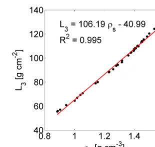
Figure 3. Relationship (red line) between soil bulk density ρs (g cm−3) and COSMIC parameterL3(g cm−2), adapted from Shut-tleworth et al. (2013). Two volcanic Hawaïan sites from Shuttle-worth et al. (2013) were discarded in this case because of their aber-rant physical characteristics.

of collisions with soil and water particles and (3) exponen-tial decay of fast neutrons while they travel upward from the place where they were created. COSMIC can be written as follows (Eq. 6):

Npih=N

∞

Z

0

e

−hms(z)

L₁ +

mw(t,z) L₂

i

· [αρs+θ (t, z)+lw+wSOM]

· 2 π ·

π 2 Z

0 e

−1 cos(β)

·

h

ms(z)

L₃ +

mw(t,z) L₄

i

dβ

dz, (6)

where β (−), L1=162.0(g cm−2), L2=129.1(g cm−2), andL4=3.16(g cm−2)are universal parameter values, and L3(g cm−2),N(cph), andα (−)are site-dependent parame-ters. The parametersmw andms are the integrated mass per unit area (g cm−2) of dry soil and water respectively andρs andρw are the dry soil bulk density and soil water density (g cm−3). In the original model, the soil water included soil moisture and lattice water (Shuttleworth et al., 2013), while Baatz et al. (2014) added soil organic matter water equivalent to this. We used an empirical relation with a high correlation (r2=0.995(−)) between parameterL3 and soil bulk den-sity (ρs) (see Fig. 3) to derive values forL3at the three sites. Hence, we calibrated only parametersNandαin this study. 2.4 Calibration methodology

sam-pling strategies (Table 1). We calibrated the parameterisa-tions, for the 1DAY strategy, for each site, for each day of the year, resulting in as many calibration solutions as there were days with data. While we could calibrate the parameterisa-tions for the 2DAY temporal strategy for all possible combi-nations of different days (65 000, 47 895, and 39 060 for SR, RB, and WB, respectively), for the higher order strategies this would, in theory, have resulted in an impractical num-ber of combinations and consequently be highly expensive computationally (Table 1). Therefore, we drew random sam-ples of day combinations, equal in size to the total number of combinations of the 2DAY strategy, from the populations of possible combinations. To investigate whether the chosen sample sizes were sufficiently large, we drew for each param-eterisation and each site, for the 4DAY and 16DAY strategies, four extra random samples of the same size. Additionally, we drew samples with different numbers of day combinations (500, 5000, 50 000, 200 000, 1 000 000) for each parameter-isation at each site. The results of both tests (not shown) in-dicated that using sample sizes of 65 000, 47 895, and 39 060 for SR, RB, and WB respectively, was sufficient for our anal-yses.

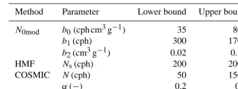
To determine parameter calibration ranges for theN0mod method, we first applied relatively wide ranges (b0: 25–1000, b1: 10–3000, and b2: 0.01–1.0) based on the original val-ues of parameters a0, a1, and a2 and values of N0 from the COsmic-ray Soil Moisture Observing System (COS-MOS) (Zreda et al., 2012; data available at http://cosmos. hwr.arizona.edu/) and Baatz et al. (2014). Using the initial ranges, we calibrated the N0mod method against soil mois-ture content – neutron intensity combinations obtained from COSMIC simulations for each of these sites. We used a range (θvarying from zero to 0.50 cm3cm−3_{increments) of} homo-geneous soil moisture profiles as input for COSMIC to calcu-late the neutron intensities for COSMOS sites from Shuttle-worth et al. (2013) (except two volcanic Hawaïan sites) and the two German sites used in this study. We used COSMIC parameter values from calibration against MCNPX (Shuttle-worth et al., 2013) for this purpose, and added the two Ger-man sites with parameter values from Baatz et al. (2014) because these showed, in contrast with the COSMOS sites, neutron intensities below 750 (cph). The resulting parameter ranges were smaller than the initial ranges and were used in our analyses (Table 3). We constructed a calibration range for HMF parameter Ns (Table 3) using the values reported by Franz et al. (2013b) and Baatz et al. (2014), and we based the parameter calibration ranges for COSMIC (Table 3) on the values found by Shuttleworth et al. (2013) and Baatz et al. (2014).

A total of 100 000 parameter sets were sampled from the parameter space of the N0mod method, 5000 for the HMF method, and 200 000 for COSMIC, using Latin hypercube sampling (LHS). We ran the parameterisations with these generated parameter sets for each day, and simulated the neu-tron intensity. We calculated the absolute error (AE) for the

Table 3. Parameter ranges for the three parameterisations used in

this study.

Method Parameter Lower bound Upper bound

N0mod b0(cph cm3g−1) 35 800

b1(cph) 300 1700

b2(cm3g−1) 0.02 0.15

HMF Ns(cph) 200 2000

COSMIC N(cph) 50 1500

α (−) 0.2 0.4

1DAY strategy, and the mean absolute error (MAE) for the multiple day strategies. The best solution for each day was found by selecting the parameter set which gave the lowest AE or MAE. To compare the overall performance through-out the whole year of a given calibrated parameterisation, we computed the MAE over all available days (with respect to simulated and observed neutron intensities) of 2012, for each best solution, hereinafter referred to as MAEval.

3 Results and discussion

3.1 Identification of strengths and weaknesses of the three parameterisations when calibrated against all available data

Figure 4. Neutron intensity time series for the calibration solutions

from the reference strategy plotted with observed neutron intensities with uncertainty bounds. The uncertainty boundaries represent 95 % confidence intervals around the mean daily fluxes. MAEvalvalues of each parameterisation are shown in the same colour used for the neutron intensity time series.

poorer results at all three sites, and COSMIC performed best at the semi-arid site, and average at the two temperate sites.

The periods of over/underestimation for all parameterisa-tions at SR could indicate either limitaparameterisa-tions with the param-eterisations used or with the quality of measurements used.

The differences between the best solutions of the three pa-rameterisations for certain periods, found at all three sites, might be related to differences in parameterisation complex-ity. Where COSMIC performed better compared to the two other methods, this could indicate the benefits of explicitly resolving individual soil layers, as opposed to using depth-weighted soil moisture as employed by the other two meth-ods. Explicitly taking into consideration the depth-varying SOM and lattice water content could potentially improve measurement depth and neutron intensity estimates.

To get a better idea of how good the best solutions from the reference strategy actually were, we compared them with calibration results obtained from previous research; see Fig. 5 and Table 4. The originalN0solution (only parameterN0 cal-ibrated) for SR was taken from the COSMOS website (Zreda et al., 2012), for HMF from Franz et al. (2013a) and for COSMIC from the MCNPx calibrations from Shuttleworth et al. (2013). We took all original solutions for RB and WB from Baatz et al. (2014). Only parameterN was calibrated for COSMIC at RB and WB (Baatz et al., 2014), while pa-rameters L3andα were computed with relationships from Shuttleworth et al. (2013). The original solutions matched the observed neutron intensities less satisfactorily when com-pared to the best solutions from the reference strategy em-ployed in this study. The most striking difference is thatN0 at SR was not able to match the observed neutron intensities

Figure 5. Neutron intensity time series for the calibration solutions

from the reference strategy (Ref.) and from original (Orig.) calibra-tion solucalibra-tions plotted together with observed neutron intensities and associated uncertainty bounds. MAEval,orig (cph) values for origi-nal solutions are included.

because of the shape of the neutron intensity–soil moisture relationship defined by parametersa0,a1, anda2(notice this was one of the main motivations for introducing the modi-fiedN0method, as discussed in Sect. 2.3.1). As mentioned in Sect. 2.3.1 for our preliminary results, this suggests that using the fixed parameter values fora0,a1, and a2 should be investigated locally. At RB the original COSMIC solution was clearly worse than our reference strategy solution and at WB this occurred for HMF and COSMIC at WB.

To identify the reasons for the relatively worse perfor-mance of the original solutions of HMF and COSMIC at RB and WB, we compared these with calibration solutions for which we used the same single days, but with our model and calibration settings (in situ soil moisture data, COS-MIC with both parametersN andαcalibrated). The differ-ences between the original and reference solution of HMF seemed to have been caused by the different values for the HMF coefficients and the chosen sampling days. The main cause for the systematic underestimations by COSMIC was that Baatz et al. (2014) calibrated only parameterN, since our solutions using the same days performed clearly bet-ter (MAEval=7.6 cph at RB; 5.0 cph at WB; compare to 12.2 cph and 9.8 cph, respectively, from the original calibra-tion).

3.2 Assessing a suitable soil sampling frequency for the three methods

Table 4. Parameter values for the best solutions of the reference strategy (Ref.) and the original (Orig.) solutions. Parametersa0, a1, anda2 are constants in the originalN0(Desilets et al., 2010) and are hence not shown. For the original HMF solutions, the coefficients used were defined by Franz et al. (2013b).

Site N0mod N0 HMF COSMIC

b0 b1 b2 N0 Ns N α L3

Ref. Orig. Ref. Orig. Ref. Orig Ref. Orig Ref. Orig

SR 122 1004 0.028 2945 870 1003 469 390 0.200 0.251 113.5 114.8

RB 61 504 0.062 1208 478 494 247 213 0.201 0.293 76.6 76.6

WB 44 384 0.021 936 706 669 195 166 0.201 0.320 50.8 50.8

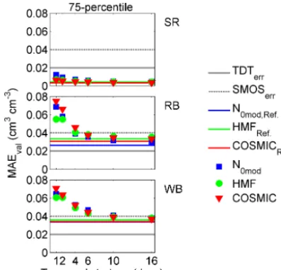
Figure 6. 25, 50, and 75 percentiles of MAEvalbest solution popu-lations. The coloured horizontal lines represent the MAEvalvalues for the calibrated solutions from the reference strategy.

horizontal lines. This figure can be interpreted as such that 25 % of the best solutions of a population had an MAEval equal to or smaller than the MAEval of the 25 percentile, the 50 % best calibration solutions had values smaller than the 50 percentile MAEval, etcetera. The MAEvalvalue of the 25 percentile hence tells us how good the better solutions were; a low value means the chance of obtaining a good solu-tion was high. A MAEvalvalue for the 75 percentile closer to the 50 and 25 percentiles means the overall range of solutions was reduced, and hence the chance of obtaining a relatively poor performance due to calibration was relatively small.

We see that for the 1DAY strategy at SR, for all three per-centiles, the MAEvalvalues ofN0modwere higher than those of HMF and COSMIC (by approximately 1.5 to 2 times). However, subsequent increase of the number of days used, made the results ofN0modapproach those of HMF. At 6DAY the MAEvalofN0modwas less than 1.2 times higher than that of HMF only. As expected, with increasing number of sam-pling days, the population range was reduced for all three parameterisations, and hence also the chance of obtaining poor solutions decreased. The differences between the tem-poral strategies were smallest for HMF at all three sites:

be-Figure 7. Soil moisture–neutron intensity relationship derived from

reference calibration for all studied sites using three distinct param-eterisations. Extrapolated curves are shown as dashed lines.

tween 1DAY and 16DAY, MAEvalvalues of HMF got up to 1.6 times smaller, while MAEvalvalues of e.g. COSMIC got up to 2.2 times smaller.

From the 75 percentiles we see that the MAEvalvalues for all three parameterisations flattened out between the 6DAY and the 10DAY strategy, after improvements of between 1.3 and 2.2 times. After these sharp decreases, little improve-ments (up to 1.2 times) were made by increasing the num-ber of days to those of the reference solutions. From a field-work perspective, this means that despite the strong increase in work effort, only a small improvement in parameterisa-tion quality will be gained. The quicker improvement (to rel-atively poor reference strategy solutions), and smaller differ-ences between the temporal strategies of HMF could be due to the fact that HMF contains only one free parameter.

Figure 8. Estimated errors in soil moisture representing the

75 percentiles obtained by calibrating against observed neutron in-tensities. The coloured horizontal lines represent the estimated er-rors from the reference strategy. The grey solid and dashed lines represent the typical errors found in point-scale sensors (TDT) and satellite remote sensing products (e.g. SMOS) respectively.

that purpose we subtracted or added the MAE neutron values from the mean observed neutron intensity and then projected onto the vertical axis of Fig. 7 to obtain soil moisture differ-ences using the reference solution curves. We did this for the 75 percentiles only. We compared them with typical errors of time domain transmissivity (TDT) sensors (0.02 cm3cm−3_, Topp et al., 2001) and with those from satellite remote sens-ing products such as SMOS and SMAP (0.04 cm3cm−3, Kerr et al., 2001). We hence assumed a 75 % chance of obtaining a calibration result, which was equal to, or better than these thresholds, sufficiently reduces the uncertainty. For simplic-ity, in order to obtain curves representing the COSMIC refer-ence solutions, we assumed homogeneous soil moisture pro-files. However, the different curves for each site had differ-ent slopes (e.g. HMF flatter at RB and WB), which would introduce mixed results not necessarily relevant to the over-all behaviour analysed for each site. We hence had to choose one curve per site to estimate soil moisture errors, shown in Fig. 8. We chose N0mod for two reasons. Firstly, it yielded the best reference solutions at RB and WB. Secondly, while COSMIC was best at SR, to obtain soil moisture error esti-mates, the need to use homogeneous profiles for this model makes representing it with a single curve an approxima-tion only. Choosing HMF or COSMIC would have yielded slightly different error magnitudes only because the curves are only slightly different within the range at which obser-vations are available for each individual site. This is indi-cated by relatively similar correlation coefficients calculated between observed and individual curves (not shown).

Figure 9. Parameter range distributions obtained for the best

so-lution populations for theN0modparameters (b0,b1, andb2). The parameter values of the reference strategy solutions are represented by black horizontal lines.

On average, all computed errors were below the two im-posed thresholds at SR. At RB and WB the magnitude of the errors was always higher than the TDT threshold. At RB, about 4 days would be needed forN0modand HMF while for COSMIC, 4 to 6 days would suffice to pass the SMOS thresh-old. All three parameterisations needed about 10 days to reach the SMOS threshold at WB. At SR, relatively low soil moisture content error estimates were obtained because the observations were limited to the dry range where the curve is relatively flat and a large neutron intensity error translates into a small soil moisture content error. At RB and WB in-stead, observed soil moisture contents were limited to the wet range and the curves are steeper than those at SR.

The distributions of the parameter values are shown in Figs. 9 and 10. The 75 percentile ranges of b0 and b1 were reduced in size by 2 to 4 times for all parameterisa-tion/site combinations with increased number of sampling days. The parameter values satisfactorily approached the so-lutions from the reference strategy (Table 4), with the excep-tion ofb2at RB and WB. Parameterb2probably specifies a soil moisture content offset at the dry end of the soil moisture content/neutron intensity curve. In Eq. (3) it is added (after multiplication withρs) to the soil moisture and lattice water terms. While at SR the observations were in the dry range, at RB and WB the wet range was observed only (Fig. 7). Hence, the role of parameterb2was probably less relevant for fitting to the data. The 75 percentile parameter ranges of HMF and COSMIC converged towards the parameter values from the reference temporal strategy for all three sites.

Figure 10. Parameter range distributions obtained for the best

solu-tion populasolu-tions for HMF parameterNsand COSMIC parameters

N, andα. The parameter values of the reference strategy solutions are represented by black horizontal lines.

bias improved (decreased) clearly with increasing numbers of sampling day, for all sites and methods (up to 20 times smaller for reference solutions compared to 1DAY),r2 re-mained nearly constant. These findings indicate that param-eterisation dynamics, which are reflected in r2, are more strongly conditioned by the input data whereas systematic biases can be caused by poor parameter selection. The found improvement of the MAEvalwith increasing number of sam-pling days was hence due to reduced systematic biases. This is important, because systematic biases in soil moisture may hinder modelling applications (e.g. data assimilation, Dee, 2005; Reichle and Koster, 2004).

Calibrating with a single day appears to be insufficient to guarantee accurate/acceptable parameterisation performance for all three parameterisations at sites enduring predomi-nantly wet soil conditions and relatively steep soil moisture content/neutron intensity curves. The results for the reference strategy and the other sampling strategies indicate thatN0mod is more easily calibrated for sites with relatively low season-ality in temperature and precipitation. HMF probably showed least differences between few and many sampling days; it only has one parameter that needs calibration. Moreover the reference strategy yielded relatively poor calibration results for HMF anyway. COSMIC performed relatively similarly for sites with different vegetation cover, and precipitation and temperature variability. A model with fewer parameters but similarly or slightly worse performance may be preferred to a more complex model.

For applications of mobile CRNS rovers (Chrisman and Zreda, 2013; Dong et al., 2014), multiple calibration in-stances are more difficult to be realised. However, in regions where stationary CRNS are available, information from mo-bile surveys can be better translated/constrained by such

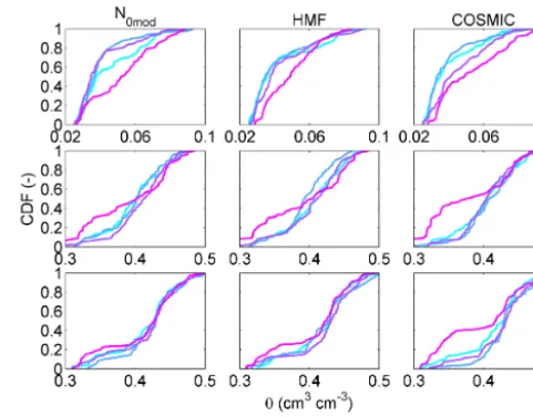
Figure 11. Cumulative density functions (CDF) of sub-groups

from the 1DAY best solution MAEvalpopulations, plotted against weighted average soil moisture content (θ) (Bogena et al., 2013).

sensors, and hence multiple-day calibration becomes even more important for stationary sensors. Alternatively, one may adopt a space-for-time approach such as those approaches proposed for satellite remote sensing soil moisture applica-tions (e.g. Reichle and Koster, 2004).

3.3 Evaluating preferred wetness conditions for calibration

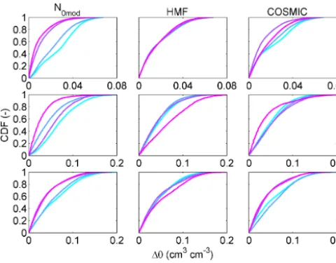
Figure 12. Cumulative density functions (CDF) of sub-groups from

the 2DAY best solution MAEvalpopulations, plotted against the dif-ference (1) between the weighted average soil moisture contents (θ) of the paired days.

The CDFs of the 1DAY strategy showed differences be-tween the 75–100 % solutions and the other groups for all site–parameterisation combinations exceptN0modand HMF at WB. At SR, relatively dry conditions seemed to yield a bet-ter chance of relatively good calibration solutions for HMF and COSMIC; for instance, 50 % (CDF=0.5(−)) of the so-lutions of the best 25 % group of both parameterisations had θ <0.035 cm3cm−3_{, while 50 % of the solutions of the worst} 25 % group hadθ >0.05 cm3cm−3_{. Relatively dry to} aver-age wetness conditions (0.03< θ <0.04 cm3cm−3_{) yielded} relatively good calibration solutions for N0mod at SR. The worst solutions (75–100 % groups) mostly originated from relatively dry conditions (θ <0.35 cm3cm−3) for all three parameterisations at RB, while the better solutions (0–75 % groups) were mostly obtained under average wetness condi-tions (0.37< θ <0.41 cm3cm−3). At WB this was only the case for COSMIC. We therefore recommend avoiding rel-atively dry conditions at RB and WB and to sample under conditions more closely related to the average conditions of those sites instead, if only a single day is used. It is unlikely that the worse calibration solutions obtained under drier con-ditions at RB and WB were caused by changes in above-ground hydrogen pools (e.g. litter layer), because Bogena et al. (2013) found that such hydrogen pools become less dominant under drier conditions.

The calibration forN0modand COSMIC at all three sites was improved when paired days with distinct soil moisture contents were used, because the CDFs of the groups of worst (50–75 and 75–100 %) calibration solutions showed rela-tively sharp increases for similar soil moisture contents (SR: 1θ <0.01 cm3cm−3; RB and WB: 1θ <0.05 cm3cm−3), whereas better solutions were obtained under relatively drier

conditions (Fig. 12). This might be expected because dif-ferent soil moisture profiles are taken into account, as well as variations in other hydrogen pools. HMF showed no dif-ferences at SR and somewhat opposite results at RB and WB, where better solutions were relatively often obtained from combinations of days with similar wetness conditions (1θ <0.05 cm3cm−3). Figures 13 (4DAY) and 14 (16DAY) show that increasing the number of days decreased the ef-fects of different wetness conditions of the constituting days. Similar to the 2DAY strategy, for the 4DAY strategy differ-ent wetness conditions were more likely to yield a relatively good calibration solution forN0modand COSMIC while for HMF, different wetness conditions seemed to affect the re-sults least.

A possible explanation for the opposite effects of wetness variability on HMF compared to the other two parameterisa-tions at RB and WB is the fixed shape of the HMF curves as shown in Fig. 7. While the shapes ofN0mod and COS-MIC can change (different parameter values) when a wider range of wetness conditions is covered, the shape of the HMF curves cannot be adjusted by sampling a wider range of wet-ness conditions and hence such practice may not always im-prove results. Figure 7 also indicates the data were limited to certain parts of the curves only and hence increasing the differences between wetness conditions outside these ranges could potentially reduce the needed number of sampling days and/or increase the confidence about the calibration results obtained.

Based on our results, we can conclude that the required number of days could be limited by choosing appropriate wetness conditions, or wetness variability. However, this is mainly limited to the worst 25 % (i.e. 75–100 %) of the anal-ysed results. The preferred choice depends on the site chosen and the parameterisation used and hence no general recom-mendation can be given.

4 Conclusions

We investigated the performance of three currently available CRNS parameterisation methods (modified N0, HMF, and COSMIC) at three sites characterised by distinct climate and land use. When calibrated with data from all days available from 1 year, the COSMIC andN0mod methods performed slightly better than HMF at the two more temperate and hu-mid sites, while at the semi-arid site, COSMIC performed better than both other methods. The soil profile approach of COSMIC gave an advantage at this site.

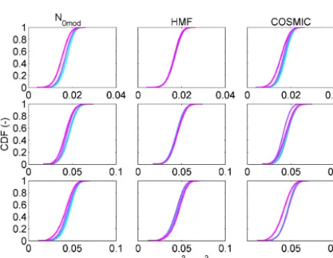
Figure 13. Cumulative density functions (CDF) of sub-groups from

the 4DAY best solution MAE_valpopulations, plotted against the SD (σ) of the weighted average soil moisture contents (θ) of the com-bined days (Bogena et al., 2013).

Figure 14. Cumulative density functions (CDF) of sub-groups from

the 16DAY best solution MAEvalpopulations, plotted against the SD (σ) of the weighted average soil moisture contents (θ) of the combined days (Bogena et al., 2013).

error is systematically below typical uncertainties observed for point-scale and satellite remote sensing products regard-less of number of sampling days. At both humid sites in Ger-many, the increase in sampling days reduced the uncertainty in translated soil moisture data to values similar or slightly below those assumed for satellite remote sensing, but failed to reach the same level of accuracy found in point-scale sen-sors.

Sampling on days or combinations of days with appropri-ate soil wetness conditions can reduce the required number of sampling days. The preferred choice depends on the site and

the parameterisation used. At the semi-arid site, theN0mod method was better calibrated better under average wetness conditions, whereas HMF and COSMIC were calibrated bet-ter under drier conditions. Average soil wetness conditions gave higher chances for better calibration results for all three parameterisations at the humid grassland site, and for COS-MIC at the humid forest site. In addition, the calibration re-sults for theN0modand COSMIC method were better when calibrated with combinations of days with distinct soil wet-ness conditions. On the other hand, HMF was less affected by distinct wetness conditions at the semi-arid site while per-forming slightly better when using days with more similar wetness conditions at both humid sites. These differences de-creased with an increasing number of days and were almost absent for the 16 days sampling strategy.

It is important to notice that varying the density and/or spa-tial (vertical and horizontal) sampling of soil moisture mea-surements may influence the calibration performance. The analysis of the actual impact on performance is beyond the scope of this study, which focuses on understanding the tem-poral sampling using typical spatial soil sampling approaches previously published in literature (Zreda et al., 2012; Desilets and Zreda, 2013; Bogena et al., 2013).

By providing a first general guideline of how often and under which wetness conditions soil moisture should be sampled, the outcomes of this study will help researchers to validate old calibration results and to reliably calibrate new CRNS sites and such as in the UK, as part of the AMUSED project (http://www.bris.ac.uk/news/2014/august/ soil-moisture-and-cosmic-rays.html). Our discussion on dif-ferences between the three CRNS parameterisation methods can be used to identify which parameterisation can be used best to relate neutron intensities to footprint average soil moisture contents.

Acknowledgements. This research was supported by the Queen’s School of Engineering (University of Bristol) PhD scholarship. Partial support for this work was also provided by the Natural Environment Research Council (A MUlti-scale Soil moisture-Evapotranspiration Dynamics study (AMUSED); grant number NE/M003086/1). We gratefully acknowledge the support from TERENO (Terrestrial Environmental Observatories) project funded by the Helmholtz-Gemeinschaft. We also thank Shirley Papuga (University of Arizona) and Trenton Franz (University of Nebraska-Lincoln) for providing data and support. We thank Robert Schwartz, Trenton Franz, Todd Caldwell, and an anony-mous reviewer for their constructive comments, which significantly improved this manuscript. Finally, the editor, Nunzio Romano, is thanked for guiding the review process.

References

Baatz, R., Bogena, H. R., Hendricks Franssen, H.-J., Huisman, J. A., Qu, W., Montzka, C., and Vereecken, H.: Calibration of a catchment scale cosmic-ray probe network: a comparison of three parameterization methods, J. Hydrol., 516, 231–244, doi:10.1016/j.jhydrol.2014.02.026, 2014.

Bogena, H. R., Huisman, J. A., Baatz, R., Hendricks Franssen, H. J., and Vereecken, H.: Accuracy of the cosmic-ray soil water content probe in humid forest ecosystems: the worst case scenario, Water Resour. Res., 49, 5778–5791, doi:10.1002/wrcr.20463, 2013. Bogena, H. R., Bol, R., Borchard, N., Brüggemann, N.,

Diekkrüger, B., Drüe, C., Groh, J., Gottselig, N., Huisman, J., Lücke, A., Missong, A., Neuwirth, B., Pütz, T., Schmidt, M., Stockinger, M., Tappe, W., Weihermüller, L., Wiekenkamp, I., and Vereecken, H.: A terrestrial observatory approach to the integrated investigation of the effects of deforestation on wa-ter, energy and matter fluxes, Sci. China Earth. Sci., 58, 61–75, doi:10.1007/s11430-014-4911-7, 2014.

Cavanaugh, M. L., Kurc, S. A., and Scott, R. L.: Evapotranspiration partitioning in semiarid shrubland ecosystems: a two-site evalu-ation of soil moisture control on transpirevalu-ation, Ecohydrology, 4, 671–681, doi:10.1002/eco.157, 2011.

Chrisman, B. and Zreda, M.: Quantifying mesoscale soil moisture with the cosmic-ray rover, Hydrol. Earth Syst. Sci., 17, 5097– 5108, doi:10.5194/hess-17-5097-2013, 2013.

Dee, D. P.: Bias and data assimilation, Q. J. Roy. Meteor. Soc., 131, 3323–3343, doi:10.1256/qj.05.137, 2005.

Demaria, E. M., Nijssen, B., and Wagener, T.: Monte Carlo sen-sitivity analysis of land surface parameters using the variable infiltration capacity model, J. Geophys. Res., 112, D11113, doi:10.1029/2006JD007534, 2007.

Desilets, D. and Zreda, M.: Footprint diameter for a cosmic-ray soil moisture probe: theory and Monte Carlo simulations, Water Re-sour. Res., 49, 3566–3575, doi:10.1002/wrcr.20187, 2013. Desilets, D., Zreda, M., and Ferré, T. P. A.: Nature’s neutron probe:

land surface hydrology at an elusive scale with cosmic rays, Water Resour. Res., 46, W11505, doi:10.1029/2009WR008726, 2010.

Dong, J., Ochsner, T. E., Zreda, M., Cosh, M. H., and Zou, C. B.: Calibration and Validation of the COSMOS Rover for Surface Soil Moisture Measurement, Vadose Zone J., 13, doi:10.2136/vzj2013.08.0148, 2014.

DWD: WebWerdis: Web-based Weather Request and Distribution System (WebWerdis) of the German Weather Service (DWD), available at: http://www.dwd.de/webwerdis, last access: 15 De-cember 2014.

Etmann, M.: Dendrologische Aufnahmen im Wassereinzugsgebiet Oberer Wüstebach anhand verschiedener Mess- und Schätzver-fahren, PhD thesis, Westfälische Wilhelms-Universität Münster, Münster, 2009.

Franz, T. E., Zreda, M., Rosolem, R., and Ferré, T. P. A.: Field val-idation of a cosmic-ray neutron sensor using a distributed sensor network, Vadose Zone J., 11, doi:10.2136/vzj2012.0046, 2012. Franz, T. E., Zreda, M., Ferré, T. P. A., and Rosolem, R.: An

as-sessment of the effect of horizontal soil moisture heterogeneity on the area-average measurement of cosmic-ray neutrons, Water Resour. Res., 49, 6450–6458, doi:10.1002/wrcr.20530, 2013a. Franz, T. E., Zreda, M., Rosolem, R., and Ferre, T. P. A.: A

uni-versal calibration function for determination of soil moisture

with cosmic-ray neutrons, Hydrol. Earth Syst. Sci., 17, 453–460, doi:10.5194/hess-17-453-2013, 2013b.

Franz, T. E., Zreda, M., Rosolem, R., Hornbuckle, B. K., Irvin, S. L., Adams, H., Kolb, T. E., Zweck, C., and Shuttle-worth, W. J.: Ecosystem-scale measurements of biomass water using cosmic ray neutrons, Geophys. Res. Lett., 40, 3929–3933, doi:10.1002/grl.50791, 2013c.

Hess, W., Canfield, E. H., and Lingenfelter, R. E.: Cosmic-ray neutron demography, J. Geophys. Res., 66, 665–677, doi:10.1029/JZ066i003p00665, 1961.

Hübner, C., Cardell-Oliver, R., Becker, R., Spohrer, K., Jotter, K., and Wagenknecht, T.: Wireless soil moisture sensor networks for environmental monitoring and vineyard irrigation, Helsinki Uni-versity of Technology, 1, 408–415, 2009.

Kerr, Y. H., Waldteufel, P., Wigneron, J.-P., Martinuzzi, J.-M., Font, J., and Berger, M.: Soil moisture retrival from space: the Soil Moisture and Ocean Salinity (SMOS) mission, IEEE T. Geosci. Remote, 39, 1729–1735, doi:10.1109/36.942551, 2001. McJannet, D., Franz, T., Hawdon, A., Boadle, D., Baker, B.,

Almeida, A., Silberstein, R., Lambert, T., and Desilets, D.: Field testing of the universal calibration function for determination of soil moisture with cosmic-ray neutrons, Water Resour. Res., 50, 5235–5248, doi:10.1002/2014WR015513, 2014.

Pelowitz, D. B.: MCNPX User’s Manual, version 2.5.0 edn., lA-CP-05-0369, Los Alamos National Laboratory, Los Alamos, New Mexico, 2005.

Qu, W., Bogena, H. R., Huisman, J. A., Martinez, G., Pachep-sky, Y. A., and Vereecken, H.: Calibration of a novel low-cost soil water content sensor based on a ring oscillator, Vadose Zone J., 12, doi:10.2136/vzj2012.0139, 2013.

Qu, W., Bogena, H. R., Huisman, J. A., Martinez, G., Pachep-sky, Y. A., and Vereecken, H.: Effects of soil hydraulic prop-erties on the spatial variability of soil water content: evidence from sensor network data and inverse modeling, Vadose Zone J., 13,doi:10.2136/vzj2014.07.0099, 2014.

Reichle, R. H. and Koster, R. D.: Bias reduction in short records of satellite soil moisture, Geophys. Res. Lett., 31, L19501, doi:10.1029/2004GL020938, 2004.

Rivera Villarreyes, C. A., Baroni, G., and Oswald, S. E.: Integral quantification of seasonal soil moisture changes in farmland by cosmic-ray neutrons, Hydrol. Earth Syst. Sci., 15, 3843–3859, doi:10.5194/hess-15-3843-2011, 2011.

Robinson, D. A., Campbell, C. S., Hopmans, J. W., Horn-buckle, B. K., Jones, S. B., Knight, R., Ogden, F., Selker, J., and Wendroth, O.: Soil moisture measurement for ecological and hydrological watershed-scale observatories: a review, Va-dose Zone J., 7, 358–389, doi:10.2136/vzj2007.0143, 2008. Rodriguez-Iturbe, I. and Porporato, A.: Ecohydrology of

Water-Controlled Ecosystems: Soil Moisture and Plant Dynamics, 1st edn., Cambridge University Press, Cambridge, United Kingdom, 2004.

Rosenbaum, U., Bogena, H. R., Herbst, M., Huisman, J. A., Pe-terson, T. J., Weuthen, A., Western, A. W., and Vereecken, H.: Seasonal and event dynamics of spatial soil moisture patterns at the small catchment scale, Water Resour. Res., 48, W10544, doi:10.1029/2011WR011518, 2012.

Hydrometeorol, 14, 1659–1671, doi:10.1175/JHM-D-12-0120.1, 2013.

Rosolem, R., Hoar, T., Arellano, A., Anderson, J. L., Shuttle-worth, W. J., Zeng, X., and Franz, T. E.: Translating aboveground cosmic-ray neutron intensity to high-frequency soil moisture pro-files at sub-kilometer scale, Hydrol. Earth Syst. Sci., 18, 4363– 4379, doi:10.5194/hess-18-4363-2014, 2014.

Scott, R. L., Cable, W. L., and Hultine, K. R.: The ecohydrologic significance of hydraulic redistribution in a semiarid savanna, Water Resour. Res., 44, W02440, doi:10.1029/2007wr006149, 1990.

Seneviratne, S. I., Corti, T., Davin, E. L., Hirschi, M., Jaeger, E. B., Lehner, I., Orlowsky, B., and Teuling, A. J.: Investigating soil moisture-climate interactions in a chang-ing climate: a review, Earth-Sci. Rev., 99, 125–161, doi:10.1016/j.earscirev.2010.02.004, 2010.

Shuttleworth, J., Rosolem, R., Zreda, M., and Franz, T.: The COsmic-ray Soil Moisture Interaction Code (COSMIC) for use in data assimilation, Hydrol. Earth Syst. Sci., 17, 3205–3217, doi:10.5194/hess-17-3205-2013, 2013.

Siebert, S., Döll, P., Hoogeveen, J., Faures, J.-M., Frenken, K., and Feick, S.: Development and validation of the global map of irrigation areas, Hydrol. Earth Syst. Sci., 9, 535–547, doi:10.5194/hess-9-535-2005, 2005.

Topp, G. C., Lapen, D. R., Young, G. D., and Edwards, M.: Eval-uation of the shaft-mounted TDT readings in disturbed and undisturbed media, Second International Symposium and Work-shop on Time Domain Reflectometry for Innovative Geotech-nical Applications. Infrastructure Technology Institute, North-western University, Evanston, Illinois, available at: http://www. iti.northwestern.edu/tdr/tdr2001/proceedings, 2001.

Topp, G. C. and Ferré, P. A.: Thermogravimetric method using con-vective oven-drying, in: Methods of Soil Analysis, edited by: Dane, J. H. and Topp, G. C., vol. Part 4: Physical Methods of Soil Science Society of America Book Series, Soil Science Soci-ety of America, Madison, Wisconsin, 422–424, 2002.

Vereecken, H., Huisman, J. A., Bogena, H., Vanderborght, J., Vrugt, J. A., and Hopmans, J. W.: On the value of soil mois-ture measurements in vadose zone hydrology: a review, Water Resour. Res., 44, W00D06, doi:10.1029/2008WR006829, 2008. Wood, E. F., Roundy, J. K., Troy, T. J., Van Beek, L. P. H., Bierkens, M. F. P., Blyth, E., De Roo, A., Döll, P., Ek, M., Famiglietti, J., Gochis, D., Van de Giesen, N., Houser, P., Jaffé, P. R., Kollet, S., Lehner, B., Lettenmaier, D. P., Peters-Lidard, C., Sivapalan, M., Sheffield, J., Wade, A., and White-head, P.: Hyperresolution global land surface modeling: meeting a grand challenge for monitoring Earth’s terrestrial water, Water Resour. Res., 47, W05301, doi:10.1029/2010WR010090, 2011. WRCC: Santa Rita Exp Range, Arizona (027593): Period of Record

Monthly Climate Summary – Temperature, available at: http: //www.wrcc.dri.edu/cgi-bin/cliMAIN.pl?azsant (last access: 16 January 2015), 2006.

Zreda, M., Desilets, D., Ferré, T. P. A., and Scott, R. L.: Measuring soil moisture content non-invasively at intermediate spatial scale using cosmic-ray neutrons, Geophys. Res. Lett., 35, L21402, doi:10.1029/2008GL035655, 2008.