CURVE FITTING: STEP-WISE LEAST SQUARES METHOD

(1)

Aryabhatta Journal of Mathematics & Informatics Vol. 6, No. 1, Jan-July, 2014 ISSN : 0975-7139 Journal Impact Factor (2013) : 0.489

-15-

CURVE FITTING: STEP-WISE LEAST SQUARES METHOD

Dhritikesh Chakrabarty

Department of Statistics, Handique Girls’ College, Guwahati – 781001, Assam, India. e-mail: [email protected], [email protected]

ABSTRACT:

A method has been developed for fitting of a mathematical curve to numerical data based on the application of the least squares principle separately for each of the parameters associated to the curve. The method has been termed as step-wise

least squares method. In this paper, the method has been presented in the case of fitting of a polynomial curve to observed

data.

Key Words : Step-wise least squares, polynomial curve, parameter estimation.

1. INTRODUCTION:

The method of least squares is indispensible and is widely used method for curve fitting to numerical data. The

method of least squares was first discovered by the French mathematician Legendre in 1805 [Mansfield (1877),

Paris (1805)]. The first proof of this method was given by the renowned statistician Adrian (1808) followed by its

second proof given by the German Astronomer Gauss [Hamburg (1809)]. Apart from these two proofs as many as

eleven proofs were developed at different times by a number of mathematicians viz. Laplace (1810), Ivory (1825),

Hagen (1837), Bassel (1838), Donkim (1844), Herscel (1850), Crofton (1870) etc.. Though none of the thirteen

proofs is perfectly satisfactory but yet it has given new dimension in setting the subject in a new light.

In fitting of a curve by the method of least squares, the parameters of the curve are estimated by solving the normal

equations which are obtained by applying the principle of least squares with respect to all the parameters associated

to the curve jointly (simultaneously). However, for a curve of higher degree polynomial and / or for a curve having

many parameters, the calculation involved in the solution of the normal equations becomes more complicated as the

number of normal equations then becomes larger. Moreover, In many situations, it is not possible to obtain normal

equations by applying the principle of least squares with respect to all the parameters jointly. These lead to think of

searching for some other method of estimating the parameters. For this reason, a new method of fitting of a curve

has been framed of which is based on the application of the principle of least squares separately for each of the

parameters associated to the curve. This paper is based on this method with respect to the fitting of a polynomial

curve.

The problem in this study can be summarized as follows:

Let the polynomial curve which is to be fitted to the n pairs of observations

(2)

Dhritikesh Chakrabarty

Y = a0 + a1X + a2X 2

+ ………. akX k

where are a0 , a1 , a2 , ……… , ak the parameters.

Then the normal equations for estimating these (k + 1) parameters obtained by applying the principle of least

squares with respect to the parameters jointly are:



 n i 1 =



 n i 1

a0 + a1 + a2

2

+ …………+ ak

k



 n i 1

= a0





n

i 1

+ a1

2

+ a2

3

+ ……… + ak

k +1



 n i 1 2

= a0





n

i 1

2

+ a1

3

+ a2

4

+ …… + ak

k +2 ………..



 n i 1 k

= a0





n

i 1

k

+ a1

k+1

+ a2

k+2

+ ……… + ak

2k

Solutions of these (k + 1) normal equations yield the least squares estimates’ of the (k + 1) parameters a0 , a1 , a2 ,

……. , ak .

Now, a method will be presented which describes how to fit the polynomial curve by applying the principle

of least squares separately for each of the parameters. The method will be called step-wise least squares method.

2. VITAL FACT - ONE THEOREM:

Let

y1 , y2 , ………. , yn

be n observations satisfying the model

yi = µ + ei (2.1)

(i = 1 , 2 , …………. , n)

where (i) µ is the true part of yi (can be called the parameter of the model)

and (ii) ei is the error associated to yi .

The problem here is to determine the least squares estimate of the true value / parameter µ.

If we want to apply the principle of least squares to estimate µ, we are to minimize S with respect to µwhere

S =



 n i1 ei 2 =



 n i1

( - µ)2 (2.2)

Minimizing S with respect to µ, the least squares estimate of µ is found as

n

1



 n i 1

yi (2.3)

Thus, the following result is obtained:

Theorem (2.1): If the observations

(3)

Curve Fitting: Step-Wise Least Squares Method

-17- satisfy the model

yi = µ + ei , (i = 1 , 2 , …………. , n)

where µ is the true part of yi and ei is the error associated to yi , then the least squares estimator of the parameter µ

is

n

1





n

i1 .

3. METHOD OF ESTIMATION OF PRAMETERS:

Suppose, the polynomial in X of degree n namely

Y = a0 + a1X + a2X 2

+ ………. + akX k

, ak ≠ 0 (3.1)

(where a0 , a1 , a2 , ………. , ak are parameters),

is to be fitted on the n pairs of observations

on (X , Y).

The problem here is to determine the parameters on the basis of the observations.

Here, the notations / operator ∆ is used to define ∆ f(xi) as

∆ f(xi) = f(xi + 1) - f(xi) .

In particular,

∆ xi = xi + 1 - xi & ∆ yi = yi + 1 - yi

i.e. ∆ operates over the suffix variable.

Also, the notation R{g(.) : h(.)} is used to describe the ratio of g(.) and h(.). For example,

R{∆ : ∆ } =

i i

x

y



Now, let

v0 = v0 (x1 , x1 , …….. , xn : y1 , y1 , ………… , yn),

v1 = v1 (x1 , x1 , …….. , xn : y1 , y1 , ………… , yn),

……….

vk = vk (x1 , x1 , …….. , xn : y1 , y1 , ………… , yn)

be the estimators of the parameters

a0 , a1 , ………. , ak

respectively obtained by the application of the principle of least squares separately for the parameters. Then the

curve, fitted by this method, will be

Y = v0 + v1X + v2X 2

+ ………. + vkX k

(3.2)

Since the n pairs of values of (X , Y) may not lie on the fitted curve, the observed values satisfy the equations

= v0 + v1 + v2 2 + ……….. + vk k + ei (3.3)

(4)

where ei is the deviation of the observed value from the corresponding value

v0 + v1 + v2 2

+ v3 3

+ ……….. + vk k

of Y yielded by the fitted curve.

This yield

∆ = v1 ∆ + v2 ∆ 2

+ v3 ∆ 3

+ ……… + vk ∆ k

+ ∆ ei

from which one obtains that

(1) = v1 + v2 2

(1) + v3

3_{(1) + ………+}

vk k

(1) + ei(1) (3.4)

where

(1) = R{∆ : ∆ } ,

r

(1) = R{∆ r : ∆ }

(r = 2 , 3 , …………. , k)

& ei(1) = R{∆ ei : ∆ }

(i = 1 , 2 , 3 , …………. , n - 1).

This again yield ∆ (1) = v2 ∆

2

(1) + v3 ∆ 3

(1) + ………….. + vk ∆ k

(1) + ∆ ei(1)

i.e. (2) = v2 + v3

3_{(2) + ………….. +}

vk k

(2) + ei(2) (3.5)

where

(2) = R{∆ (1) : ∆ 2(1)} ,

r

(2) = R{∆ r(1) : ∆ 2(1)}

(r = 3 , 4 , …………. , k)

& ei(2) = R{∆ei(1) : ∆ 2(1)}

(i = 1 , 2 , 3 , …………. , n - 2).

This further yield

∆ (2) = v3 ∆ 3(2) + ………….. + vk ∆ k(2) + ∆ ei(2)

i.e. (3) = v3 + v4 4(3) + ………….. + vk k(3) + ei(3) (3.6)

where

(3) = R{∆ (2) : ∆ 3(2)} ,

r

(3) = R{∆ r(2) : ∆ 3(2)}

(r = 4 , 5 , …………. , k)

& ei(3) = R{∆ei(2) : ∆ 3(2)}

(i = 1 , 2 , 3 , …………. , n - 3).

At the sth step, one obtains that

∆ (s - 1) = v3 ∆ 3(s - 1) + ………… + vk ∆ k(s - 1) + ∆ ei(s - 1)

i.e. (s) = vs + vs + 1 s+ 1(s) + ………… + vk k(s) + ei(s) (3.7)

where

(s) = R{∆ ( s - 1) : ∆ 3(s - 1)} ,

r

(5)

-19- (r = s + 1 , s + 2 , …………. , k)

& ei(s) = R{∆ei(s - 1) : ∆ 3

(s - 1)}

(i = 1 , 2 , 3 , …………. , n - s).

At the (k



1)th step, one obtains that ∆ (k - 2) = vk - 1 ∆

k - 1

(k - 2) + vk ∆ k

(k - 2) + ∆ ei(k - 2)

i.e. ( k - 1) = v k - 1 + vk k

(k - 1) + ei(k - 1) (3.8)

where ( k - 1) = R{∆ (k - 2) : ∆ k - 1(k - 2)}

& ei(k - 1) = R{∆ ei(k - 2) : ∆ k - 1

(k - 2)}

(i = 1 , 2 , 3 , …………. , n – k + 1).

Finally, at the kth step one obtains that ∆ (k - 1) = vk ∆

k

(k - 1) + ∆ ei(k - 1)

i.e. (k) = vk + ei(k) (3.9)

where (k) = R{∆ (k - 1) : ∆ k(k - 1)}

& ei(k) = R{∆ ei(k - 1) : ∆ k

(k - 1)}

(i = 1 , 2 , 3 , …………. , n - k).

This is of the form (2.1).

Therefore by Theorem (2.1),

vk = vk (x1 , x1 , …….. , xn : y1 , y1 , ………… , yn)

=

k

n



1



 

k n

i1

(k) (3.10)

Also from (3.8), one obtains that

(k - 1) - vk k

(k - 1) = v k - 1 + ei(k - 1) (3.11)

This is also of the form (2.1).

Therefore by the same theorem,

vk - 1 = vk – 1 (x1 , x1 , …….. , xn : y1 , y1 , ………… , yn)

=

1

1 



k

n



 



1

1 k n

i

{ ( k - 1) - vk k

(k - 1)} (3.12)

Similarly from the equation obtained at the (k



2)th step, one obtains that

(k - 2) - vk - 1 k - 1

(k - 2) - vk k

(k - 2) = vk - 2 + ei(k - 2) (3.13)

This is also of the form (2.1).

Therefore by the same theorem,

vk - 2 = vk – 2 (x1 , x1 , …….. , xn : y1 , y1 , ………… , yn)

=

2

1 



k

n



 



2

1 k n

i

{ (k - 2) - vk - 1

k - 1

(k - 2) - vk k

(k - 2)} (3.14)

Applying the same technique at the earlier steps successively, one can obtain the estimators of the parameters as

follows:

(6)

Dhritikesh Chakrabarty =

s

n



1



  s n i 1

{ (s) - vs + 1 s+ 1

(s) - vs + 2 s+ 2

(s) - ……. - vk k

(s)} (3.15)

vs- 1 = v s- 1 (x1 , x1 , …….. , xn : y1 , y1 , ………… , yn)

=

1

1 



s

n



   1 1 s n i

{ (s - 1) - vs s

(s - 1) - vs + 1 s+ 1

(s - 1) - ……….

……. - vk k

(s - 1)} (3.16)

v1 = v1 (x1 , x1 , …….. , xn : y1 , y1 , ………… , yn)

=

1

1 

n



  1 1 n i

{ (1) - v2 2

(1) - v3 3

(1) - ……. - vk k

(1)} (3.17)

v0 = v0 (x1 , x1 , …….. , xn : y1 , y1 , ………… , yn)

=

n

1



 n i 1

{ - v1 - v2 2

- ……… - vk k

} (3.18)

Note:

In this method, the estimates of the parameters are to be computed in the following order:

First, estimate vk of the parameter ak ,

Then, estimate vk - 1 of the parameter ak – 1 ,

………

next, estimate vs of the parameter as ,

next, estimate vs- 1 of the parameter as- 1 ,

………...

next, estimate v1 of the parameter a1 ,

finally, estimate v0 of the parameter a0 .

Special Cases

Case -1 (Fitting of a linear curve):

If the curve Y = f(X) is linear of the form

Y = a0 + a1X (3.19)

where a0 & a1 are the parameters, the estimators

v0 = v0 (x1 , x1 , …….. , xn : y1 , y1 , ………… , yn)

& v1 = v1 (x1 , x1 , …….. , xn : y1 , y1 , ………… , yn)

of the parameters a0 & a1 respectively will be as follows:

v1 =

1

1 

n



  1 1 n i

(1) (3.20)

& v0 =

n

1



 n i 1

(



v1 ) (3.21)

(7)

-21-

Case - 2 (Fitting of a quadratic curve):

Y = a0 + a1X + a2X 2

(3.22)

where a0 , a1 & a2 are the parameters, the estimators

v0 = v0 (x1 , x1 , …….. , xn : y1 , y1 , ………… , yn),

v1 = v1 (x1 , x1 , …….. , xn : y1 , y1 , ………… , yn)

& v2 = v2 (x1 , x1 , …….. , xn : y1 , y1 , ………… , yn)

of the parameters a0 , a1 & a2 respectively will be as follows:

v2 =

2

1 

n



  2 1 n i

(2) (3.23)

v1 =

1

1 

n



  1 1 n i

{ (1)



v2 2

(1)} (3.24)

v0 =

n

1



 n i1

{



v1



v2 2} (3.25)

where (1) = R{∆ : ∆ }, (i = 1 , 2 , 3 , ……… , n – 1),

2

(1) = R{∆ 2 : ∆ }, (i = 1 , 2 , 3 , ……… , n – 1)

& (2) = R{∆ (1) : ∆ 2(1)} , (i = 1 , 2 , 3 , ……… , n – 2).

Case - 5 (Fitting of a cubic curve):

Y = a0 + a1X + a2X 2

+ a3X 3

(3.26)

where a0 , a1 , a2 & a3 are the parameters, the estimators

v0 = v0 (x1 , x1 , …….. , xn : y1 , y1 , ………… , yn),

v1 = v1 (x1 , x1 , …….. , xn : y1 , y1 , ………… , yn),

v2 = v2 (x1 , x1 , …….. , xn : y1 , y1 , ………… , yn)

& v3 = v3 (x1 , x1 , …….. , xn : y1 , y1 , ………… , yn)

of the parameters a0 , a1 , a2 & a3 respectively will be as follows:

v3 =

3

1 

n



  3 1 n i

(3) (3.27)

v2 =

2

1 

n



  2 1 n i

{ (2) - v3 3(2)} (3.28)

v1 =

1

1 

n



  1 1 n i

{ (1) - v 2 2

(1) - v3 3

(8)

Dhritikesh Chakrabarty v0 =

n

1





n

i 1

( yi - a0 - a1xi - a2xi 2

- a3xi 3

) (3.30)

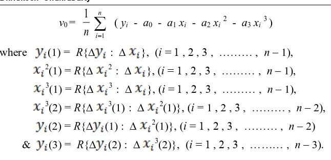
where (1) = R{∆ : ∆ }, (i = 1 , 2 , 3 , ……… , n – 1),

2

(1) = R{∆ 2 : ∆ }, (i = 1 , 2 , 3 , ……… , n – 1),

3(1) = R{∆ 3 : ∆ }, (i = 1 , 2 , 3 , ……… , n – 1),

3

(2) = R{∆ 3(1) : ∆ 2(1)}, (i = 1 , 2 , 3 , ……… , n – 2),

(2) = R{∆ (1) : ∆ 2(1)}, (i = 1 , 2 , 3 , ……… , n – 2)

& (3) = R{∆ (2) : ∆ 3(2)}, (i = 1 , 2 , 3 , ……… , n – 3).

4. NUMERICAL EXAMPLES:

Example 4.1: Consider the problem of fitting of the linear curve

Y = a0 + a1X

(where a0 & a1 are the parameters)

to the following observations on X and Y:

xi : 0 5 7 10 16 20 21 25 31 40

yi : 2 17 24 33 51 63 64 76 94 123

In order to determine the estimates of a0 & a1, the following table (Table - 4.1) is to be prepared:

Table-4.1

(1) (2) (3) (4) (5) (6)

∆ ∆ (1)



v1 with

v1 = 3.001234568

0 2 5 17 3.4 -1.001234568

5 17 2 7 3.5 1.993827160

7 24 3 9 3 2.991358024

10 33 6 18 3 2.987654320

16 51 4 12 3 2.980246912

20 63 1 2 2 2.975308640

21 65 4 12 3 1.974074072

25 77 6 18 3 1.969135800

31 95 9 28 3.1111111 1.961728392

40 123 2.950617280

Total

= 175

Total

= 550

Total

=27.0111111

Total

= 24.78305064

Now, v1 =

9

1





9

1 i

(9)

-23-

& v0 =

10

1





10

1 i

(



v1 ) = 2.478305064

Thus the linear curve fitted to the observations becomes

Y = 2.478305064 + 3.001234568 X

Example 4.2: Consider the problem of fitting of the quadratic curve

Y = a0 + a1X + a2X 2

(where a0 . a1 & a2 are parameters)

to the following observations on X and Y:

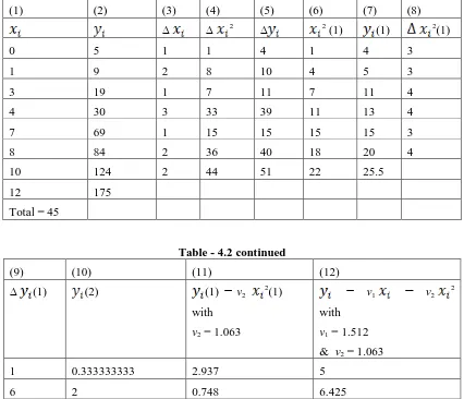
xi : 0 1 3 4 7 8 10 12

yi : 5 9 19 30 69 84 124 175

In order to determine the estimates of a0 , a1 & a2 , the following table (Table - 4.2) is to be prepared:

Table - 4.2

(1) (2) (3) (4) (5) (6) (7) (8)

∆ ∆ 2 _∆ 2

(1) (1) 2(1)

0 5 1 1 4 1 4 3

1 9 2 8 10 4 5 3

3 19 1 7 11 7 11 4

4 30 3 33 39 11 13 4

7 69 1 15 15 15 15 3

8 84 2 36 40 18 20 4

10 124 2 44 51 22 25.5

12 175

Total = 45

Table - 4.2 continued

(9) (10) (11) (12)

∆ (1) (2) (1)



v2

2

(1)

with

v2 = 1.063



v1



v2

2

with

v1 = 1.512

& v2 = 1.063

1 0.333333333 2.937 5

6 2 0.748 6.425

2 0.5 3.559 4.897

(10)

5 1.666666666 - 0.945 6.329

5.5 1.375 0.866 3.872

2.114 2.588

3.784

Total = 6.375 Total = 10.586 Total = 39.839

Now, v2 =

6

1





6

1 i

(2) _{= 1.063 ,}

v1 =

7

1





7

1 i

{ (1)



v2 2

(1)} = 1.512

& v0 =

8

1





8

1 i

( yi - a0 - a1xi - a2xi2 - a3xi3 ) = 4.98

Thus the quadratic curve fitted to the observations becomes

Y = 4.98 + 1.512 X + 1.063 X2

5. CONCLUSION:

(1) The method developed in this paper is based on the application of the principle of least squares with respect

to the parameters separately while the usual method of least squares is based on the application of the

principle of least squares with respect to the parameters jointly.

(2) The method is suitable for fitting of a polynomial curve of any finite order.

(3) It is yet to be investigated whether this method can be applicable to a curve other than polynomial curve

to observed values.

(4) It is yet to be searched for whether the estimates of parameter obtained by this method and those obtained by

solving the normal equations of the curve under study are identical.

6. REFERENCE:

1. AdrianA. (1808): “ The Analyst ”, No.- IV, 93-109.

2. Bessel (1838): “ On utersuchungen ueber die Wahrscheinlichkeit der Beobachtungsfehler ”.

3. Crofton (1870): “ On the Proof of the Law of Error of Observations”, Phil. Trans, London, 175-188.

4. Donkin (1844): “ An Essay on the Theory of the Combination of Observations ”, Joua. Math., XV,

297-322.

4. Gauss C. F. (1809): “ Theory of Motion of Heavenly Bodies ”, Humburg , 205-224.

6. Hagen (1837): “ Grandzuge der Wahrscheinlichkeitsrechnung ”, Berlin.

7. Herschel J. (1850): “ Quetelet On Probabilities ”, Edinburgh Review, XCII, 1-57.

8. Ivory (1825): “ On the Method of Least Squares ”, Phil. Mag., LX, 3-10.

9. Koppelmann R. (1971): “ The Calculus of Operation ”, History of Exact Sc., 8, 152-242.

(11)

-25- 11. Merriman M. (1877): “ The Analyst ”, Vol. -IV, NO-2.

12. D. Chakrabarty [2010] “Probability as the Maximum Occurrence of Relative Frequency” Aryabhatta J. of

Maths & Info., Vol. 2 [2], pp 339-344.

13. D. Chakrabarty [2013] “One Table of Three Digit Random Numbers” Aryabhatta J. of Maths & Info., Vol. 5