The design and implementation of a Bayesian CAD modeler for
robotic applications
K. MEKHNACHA
∗E. MAZER
†P. BESSI `
ERE
‡Abstract
We present a Bayesian CAD modeler for robotic applications. We address the problem of taking into account the propagation of geometric uncertainties when solving inverse geometric problems. The proposed method may be seen as a generalization of constraint-based approaches in which we explicitly model geometric uncertainties. Using our methodology, a geometric constraint is expressed as a probability distribution on the system parameters and the sensor measurements, instead of a simple equality or inequality. To solve geometric problems in this framework, we propose an original resolution method able to adapt to problem complexity. Using two examples, we show how to apply our approach by providing simulation results using our modeler.
Keywords: Robotics, CAD, Bayesian reasoning, Monte Carlo methods, geometric constraints.
1
Introduction
The use of geometric models in robotics and CAD systems necessarily requires a more or less realistic modeling of the environment. However, the validity of calculations with these models depends on their degree of fidelity to the real environment and the capacity of these systems to represent and take into account possible differences between the models and reality when solving a given problem.
This paper presents a new methodology based on Bayesian formalism to represent and handle geometric uncertainties in robotics and CAD systems. The approach presented in this paper may be seen as a generalization of constraint-based approaches. This generalization consists of explicitly taking into account the uncertainties in models. A constraint on a relative pose between two frames is represented by a probability distribution on the parameters of this pose instead of simple equality or inequality. In this framework, modeling information given by the programmer and the measurements obtained using sensors are represented and used in a homogeneous way. For a given problem, all the information we include on the geometric model and on the responses of the sensors used, is used optimally applying Bayesian reasoning.
Since the work of Laplace [Laplace, 1774], numerous results have been obtained using Bayesian inference techniques to take account of uncertainty. Bayesian formalism has been applied in diverse research fields. Numerous applications have been developed in physics [Jaynes, 1996, Neal, 1993], in artificial intelligence [Jaakkola and Jordan, 1999], as well as in mobile robotics [Thrun, 1998, Bessi`ere et al., 1998] and computer vision [Weiss and Adelson, 1998], and especially in parameter identification problems [Presse and Gautier, 1992].
The principle of the proposed method is to infer, for a given problem, the marginal distribution of the unknown parameters using the probability calculus. The original geometric problem is reduced to an optimization problem over the marginal distribution to find a solution with maximum probability. In the general case, this marginal probability may contain an integral on a large dimension space.
The resolution method used to solve this integration/optimization problem is based on an adaptive genetic algorithm. The problem of integral numerical estimation is approached using a stochastic Monte Carlo method. The accuracy of this estimation is controlled by the optimization process to reduce computation time.
A large category of robotic applications are instances of inverse geometric problems in the presence of un-certainties, for which our method is well suited. The simplicity of our specification method and the robustness of our resolution method make our approach applicable to numerous robotic applications [Mekhnacha, 1999, Mekhnacha et al., 2000], such as:
• kinematics inversion under geometric uncertainties using possibly redundant mechanisms,
• robot and sensor calibration,
• parts’ pose and shape calibration using sensor measurements,
• robotic workcell design to obtain a configuration that can accomplish a given task with maximum accuracy.
Extensive experimentation on the approach was made possible thanks to the design and the implementation of a Bayesian CAD modeler. Experimental results obtained with this modeler have demonstrated the effectiveness and the robustness of our approach. Two examples of this experimentation are presented in this paper.
This paper is organized as follows. We first report related work in Sect. 2. In Sect. 3 we present our specification methodology and show how to formulate an optimization problem. In Sect. 4 we describe our numerical resolution method. Section 5 is an overview of the implementation of our modeler. We present two examples to illustrate our approach in Sect. 6 and Sect. 7 and give some conclusions and perspectives in Sect. 8.
This paper summarizes the work presented in the Ph.D. thesis of Kamel Mekhnacha [Mekhnacha, 1999].
2
Related work
The representation and handling of geometric uncertainties is a central issue in the fields of robotics and mechanical assembly. Since the precursor work of Taylor [Taylor, 1976], in which geometric uncertainties were taken into account in the robot manipulators planning process, numerous approaches have been proposed to model these uncertainties explicitly.
Methods modeling the environment using “certainty grids” [Moravec, 1988] and those using uncertain models of motion [Lozano-P`erez, 1987, Alami and Simeon, 1994] have been used extensively, especially in mobile robotics. Gaussian models to represent geometric uncertainties and to approximate their propagation have been pro-posed in manipulator programming [Puget, 1989] as well as in assembly [Sanderson, 1997]. Kalman filtering is a Bayesian recurrent implementation of these models. This technique has been used widely in robotics and vision [Zhang and Augeras, 1992] and particularly in data fusion [Bar-Shalom and Fortmann, 1988]. Gaussian model-based methods have the advantage of economy in the computation they require. However, they are only applicable when a linearization of the model is possible. Another limitation of these methods is their inability to take account of inequality constraints.
Geometric constraint-based approaches [Taylor, 1976, Owen, 1996] using constraint solvers have been used in robotic task-level programming systems. Most of these methods do not represent uncertainties explicitly. They handle uncertainties using a least-squares criterion when the solved constraints systems are over-determined. In the cases where uncertainties are explicitly taken into account (as is the case in Taylor’s system), they are described solely as inequality constraints on possible variations.
3
Specification of probabilistic geometric constraints
In this section, we describe our methodology by giving some concepts and definitions necessary for probabilistic geometric constraint specification. We further show how to derive an objective function to maximize from the original geometric problem.
3.1
Probabilistic kinematic graph
S1 S2
k−1
S S
4
Sk S3
Oi
Ci
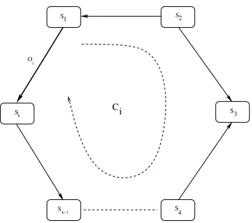
Figure 1: Example of a cycle in the kinematic graph.
• a modeling constraint (a piece of knowledge) on the relative pose of the parent frame and its child,
• a sensor measurement of the pose of a given entity,
• or a constraint we wish to satisfy to solve the problem (an objective value with a given precision, for example).
Each edge Aikjk is labeled by:
1. a probability distribution p(Qikjk) where Qikjk is the relative pose vector (six-vector) Qikjk = (txtytzrxryrz)T. The first three parameters of this six-vector represent the translation, while the remaining
three represent the rotation.
2. possible equality/inequality constraints (Ek(Qikjk) = 0,Ck(Qikjk)≤0). These constraints represent possi-ble geometric relationships between the two geometric entities attached to these two frames. Their shapes depend on the type of the geometric relationship. We implement several relationships between geomet-ric entities in this work, such as points, polygonal faces, edges, spheres and cylinders. The details on equality/inequality constraints induced by these relationships can be found in [Mekhnacha, 1999].
3. a “status” six-vector describing for each parameter ofQikjk, its role (nature) in the problem. A status can take one of the three following values:
• Unknown(denoted by X) for parameters representing the unknown variables of the problem and whose values must be found to solve the problem.
• Free(denoted by L) for parameters whose values are only known with a probability distribution. This allows to express uncertainties on the model.
• Fixed(denoted by F) for parameters having known fixed scalar values that cannot be changed. In the general case, the kinematic graph may contain a set of cycles. The presence of a cycle represents the existence of more than one path between two vertices (frames) of the graph. To ensure the geometric coherence of the model, the computation of the relative pose between these two frames using all paths must give the same value. For each cycle containing kedges (see Fig. 1), we have:
TSiSi=T
dSiSi+1 SiSi+1 ∗T
dSi+1Si+2
Si+1Si+2 ∗ · · · ∗T
dSk
−1Sk
Sk−1Sk ∗
TdSkS1
SkS1 ∗T
dS1S2
S1S2 ∗ · · · ∗T
dSi
−1Si
Si−1Si =I4, (1)
where Tij is the 4×4 homogeneous matrix corresponding to the pose vectorQij,I4 is the 4×4 identity matrix
anddij ∈ {−1,1}is the direction in which the edgeAij has been used.
3.2
Objective function
Given a probabilistic kinematic graph, we are interested in constructing a marginal distribution over the unknown parameters (parameters having the unknownstatus) of the problem. Maximizing this distribution will provide a solution to the problem.
We define the following sets of propositions:
• A set ofppropositions{Ki} p
i=1 such as: Ki≡“cycleci is closed”.
• A set ofmpropositions{Hk}mk=1 such as: Hk≡“Ck(Qikjk)≤0 andEk(Qikjk) = 0”.
If we denote the unknown parameters of the problem by X, a solution to a problem is a value of X that maximizes the marginal distribution
p(X|H1· · · HmK1· · · Kp).
If we denote by L0 the concatenation of the parameters having status L and by X the concatenation of the
parameters having status X, we can write using the probability calculus:
p(X|H1· · · HmK1· · · Kp) ∝
Z
dL0 p(XL0H
1· · · HmK1· · · Kp)
= p(X) Z
dL0 p(L0)p(H
1· · · HmK1· · · Kp|XL0).
To use the global equality constraints (Eq. 1), we take for each cycle ci, i= 1· · ·pa pose vector we rename
Oi (Fig. 1). This pose vector is chosen so that it contains no parameters having the X status. Equation 1 allows
us to compute the value of Oi using the values of all the other pose vectors pertaining toci:
Oi = QS1Sk
= Fi QS1S2, QS2S3,· · ·, QSk−1Sk
= vect(mat(QS1S2))
dS1S2∗(mat(Q
S2S3))
dS2S3∗ · · · ∗ mat(Q
Sk−1Sk)
dSk
−1Sk
,
where
• vectis the function allowing to get a pose vector from the corresponding 4×4 homogeneous matrix,
• matis the function allowing to get a 4×4 homogeneous matrix from the corresponding pose vector,
• dij∈ {1,−1}denotes the direction in which the edgeAij has been used.
Using this equality constraint cancels the integrals over the parameters of L0 that pertain to Oi, because the
integrand takes a non-null value only for the point that respect Eq. 1.
For each edgeAij, if we denote byLijthe set of parameters having status L and byXij the parameters having
status X, we can write, using appropriate independence assumptions, the following general form:
p(X|H1· · · HmK1· · · Kp)∝p(X)I(X),
where
I(X) = Z
dL
p(Li1j1)p(H1|Xi1j1Li1j1)
.. .
p(Lim−pjm−p)p(Hm−p|Xim−pjm−pLim−pjm−p)
pO1(F1(X, L))p(Hm−p+1|F1(X, L))
.. .
For each cycle ci, i = 1· · ·p, pOi denotes the distribution over Oi, while L ⊂ L0 is the concatenation of
Li1j1,· · ·, Lim−pjm−p.
The distributionp(X) is called thea prioridistribution over the unknown parametersX (before incorporating the constraints), while the distribution p(X|H1· · · HmK1· · · Kp) is called the a posteriori distribution over X
(after incorporating the constraints).
For eachAikjk, k= 1,· · ·, m−p, marginalizing (by integration) over the free parametersLikjk allows to take into account the propagation of the uncertainties expressed using the distribution p(Likjk)corrected using the local constraintsHk.
Maximizing the a posteriori distribution p(X|H1· · · HmK1· · · Kp) provides the “Maximum A Posteriori”
(MAP) solution of the problem.
4
Resolution method
We described in the previous section how to express a geometric problem as an integration/optimization problem:
X∗= max
X [p(X|H1· · · HmK1· · · Kp)].
In this section, we will present the practical numerical methods we used to solve these two problems.
4.1
Numerical integration method
Integral calculus is the basis of Bayesian inference. Unfortunately, analytic methods for integral evaluation seem very limited in real-world applications, where integrands may have complex shapes and integration spaces may have very high dimensionality.
Domain subdivision-based methods (such as trapezoidal or Simpson’s methods) are often used for numerical integration in low-dimensional spaces. However, these techniques are poorly adapted for high-dimensional cases.
4.1.1 Monte Carlo methods for numerical estimation
Monte Carlo (MC) methods are powerful stochastic simulation techniques that may be applied to solve opti-mization and numerical integration problems in large dimensional spaces. Since their introduction in the physics literature in the 1950s, Monte Carlo methods have been at the center of the recent Bayesian revolution in applied statistics and related fields, including econometrics [Geweke, 1996] and biometrics. Their application in other fields such as image synthesis [Keller, 1996] and mobile robotics [Dellaert et al., 1999] is more recent.
Principles
The principle of using Monte Carlo methods for numerical integration is to approximate the integral
I = Z
f(l)g(l)ddl,
by estimating the expectation of the function g(l) under the distributionf(l)
I = Z
f(l)g(l)ddl=hg(l)i.
Suppose we are able to obtain a set of samples {l(i)}N
i=1 (d-vectors) from the distribution f(l). We can use
these samples to derive the estimator
ˆ
I = 1
N
X
i
g(l(i)).
Clearly, if the vectors {l(i)}N
i=1 are generated fromf(l), the variance of the estimator ˆI = N1
P
ig(l(i)) will
decrease as σ2
N, whereσ
2 is the variance ofg:
σ2= Z
and ˆg is the expectation ofg.
This result is one of the important properties of Monte Carlo methods:
“The accuracy of Monte Carlo estimates is independent of the dimensionality of the integration space”.
4.1.2 Using MC methods for our application
Using an MC method to estimate the integral (2) requires the following steps.
1. Sample a set ofN points {L(i)}N
i=1 from the prior distributionp(L) such that the sampled points respect
local equality/inequality constraints (i.e.,{Hi} m−p
i=1 have the valuetrue).
2. Estimate the integralI(X) using the set{L(i)}N
i=1 of points as follows.
ˆ
I(X) = 1
N
N
X
i=1
pO1(F1(X, L
(i)))
p(Hm−p+1|F1(X, L(i)))
.. .
pOp(Fp(X, L
(i)))
p(Hm|Fp(X, L(i))).
Points sampling
The set ofN points used to estimate the integral may be sampled in various ways. Since parameters pertaining to different pose vectors are independent, we can decompose the “state vector”Ltom−pcomponents{Likjk}
m−p k=1
and apply a local sampling algorithm [Geweke, 1996, Neal, 1993]. Using a local sampling algorithm, updating the state vectorL
L(t)= (L(t)
i1j1, L
(t)
i2j2,· · ·, L
(t)
ikjk,· · ·, L
(t)
im−pjm−p)
only requires updating one component Likjk
L(t+1)= (Li(1t)j1, L(i2t)j2,· · ·, L(ikt+1)jk ,· · ·, L(itm)
−pjm−p).
N iterations of this procedure give us the set{L(i)}N
i=1, which will be used to estimate the integral.
To update a component Likjk (a set of parameters pertaining to the same pose vector Qikjk), we must take into account possible dependencies between these parameters. Consequently, we face two problems.
• Candidate point sampling
A candidate Lc
ikjk is drawn from the distribution p(Likjk). Direct sampling methods from simple distri-butions such as uniform distridistri-butions and Gaussians are available. If we do not have a direct sampling method fromp(Likjk) at our disposal, an indirect sampling method must be used. In this work, we chose a Metropolis sampling algorithm [Geweke, 1996, Neal, 1993].
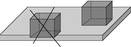
• Candidate validity checking
Suppose we have a geometric relationship between two geometric entitiesEiandEj. A geometrical calculus
depending on the type of this relationship allows checking of the constraintCk(Qikjk)≤0. If this constraint is respected (i.e.,p(Hk|XikjkLikjk) = 1), the candidateL
c
ikjk is accepted, otherwise it is rejected. Figure 2 shows aFace-On-Facerelationship example.
Optimization of computation time
Using a local sampling method to update the state vector Lallows a reduction in the computation time of the estimates of integrals. If, for a given pointL(t), we denote the values of functionsF
i(X) byF( t)
i (X), i= 1· · ·p,
then the values of Fi(X) in the next stepF
(t+1)
i (X) are obtained by partly updatingF
(t)
Figure 2: The candidate point is rejected because it does not respect theFace-On-Faceconstraint.
4.2
Optimization method
The optimization method to be chosen for our application must satisfy a set of criteria in relation to the shape and nature of the function to optimize. The method must:
1. be global, because the function to optimize is often multimodal,
2. allow multiprecision computation of the objective function. Its estimation with high accuracy may require long computation times,
3. allow parallel implementation to improve efficiency.
For our application, we chose a genetic algorithm that satisfies these criteria. First, we present the general principles of these algorithms. Then, we discuss the practical problems we faced when using standard genetic algorithms in our application and give the required improvements.
4.2.1 Principles of Genetic Algorithms
Genetic algorithms (abbreviated GA) are stochastic optimization techniques inspired by the biological evolution of species. Since their introduction by Holland [Holland, 1975] in the seventies, these techniques have been used for numerous global optimization problems, thanks to their ease of implementation and their independence of applica-tion fields. They are widely used in a large variety of domains including artificial intelligence [Grefenstette, 1988] and robotics [Mazer et al., 1998].
The goal of a GA is to find a global optimum of a given function F over a search spaceS.
During an initialization phase, a set of points (individuals) are drawn at random from the search spaceS that is discretized with a given resolution. This set of points is called a population.
Each individual I is coded by a string of bits. It represents a solution of the problem and its adequacy is measured by a value F(I).
The fundamental principle of genetic algorithms is: “the better the adequacy of an individual, the larger is the probability of selecting it for reproduction”. “Genetic operators” are applied to the selected individuals to generate new ones. For a given size of population, better individuals obtained by reproduction replace initial ones. This process is iterated until a convergence criterion is reached.
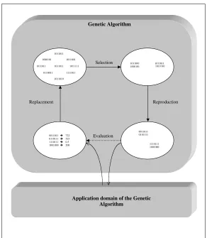
The standard sequential genetic algorithm can be described as follows. First, an initial population is drawn at random from the search space and the following cycle is then performed (see Fig. 3).
1. Selection: Using the functionF, pairs of individuals are selected. The probability of selecting an individual
I grows with the value ofF(I) for this individual.
2. Reproduction: Genetic operators are applied to the selected individuals to produce new ones.
3. Evaluation: The values ofF are computed for the new individuals.
4. Replacement: Individuals in the current population are replaced by better new individuals.
1011001 1011011
1011011 1011011 1000101
0110011
1011111
1111011
1011010
1011001
1000101 10110111011010
0011011è722 0110111è525 1110111è0.5 1001000è200
0011011 0110111
1110111 1001000 Selection
Evaluation
Reproduction Replacement
Application domain of the Genetic Algorithm
Genetic Algorithm
Figure 3: Genetic Algorithm iterations.
In this work, we use a population with a constant size of 100 individuals. We discretize the search space with a resolution of 10−4 rad for orientation parameters and of 10−3 mm for translation ones. For example,
an orientation parameter that takes a value between 0.0 and 2π rad (discretized with a 10−4 rad resolution) is
coded on a 16 bits string (0.0 ≡00· · ·0 | {z }
16
, while 2π ≡11· · ·1 | {z }
16
). A string coding a given configuration is simply
the concatenation of the strings codings each parameter. For reproduction, we use both the cross-over and the mutation operators. First, we use the cross-over operator to get an intermediate individual (string). Then, the mutation operator is applied with a probability of 0.2 on this intermediate individuals to get the final individuals.
In the following, we will useG(X) to denote the objective functionp(X|H1· · · HmK1· · · Kp).
4.2.2 Narrowness of the objective function - constraint relaxation
In our applications, the objective function G(X) may have a narrow support (the region where the value is not null) for very constrained problems. The initialization of the population with random individuals from the search space may give null values of the function G(X) for most individuals. This will make the evolution of the algorithm very slow and its behavior will be similar to random exploration.
To deal with this problem, a concept inspired from classical simulated annealing algorithms consists of intro-ducing a notion of “temperature”. The principle is to first widen the support of the function by changing the original function to obtain non-null values even for configurations that are not permitted. To do so, we introduce an additional parameter we call T (for temperature) for the objective function G(X). Our goal is to obtain another function GT(X) that is smoother and has wider support, with
lim
T→0G
T(
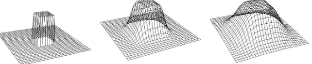
Figure 4: The distribution corresponding to inequality constraints induced by aPoint-On-Face relationship for a square face at different values of temperature. The left figure shows the original constraints (T = 0), while the middle and the right ones show these constraints relaxed at (T = 50) and (T = 100) respectively.
To widen the support of G(X), all elementary terms (distributions) ofG(X) are widened, namely:
• distributionspOi(Fi(X, L)), wherei= 1· · ·p.
• inequality constraintsp(Hm−p+j|Fj(X, L)), wherej= 1· · ·p.
For example:
• for a Gaussian distribution:
f(x) = √1
2πσe
−12 (x−µ)2
σ2
fT(x) = √ 1
2πσ(1 +T)e
−12 (x−µ)2
[σ(1+T)]2
• for an inequality constraint over the interval [a, b]:
f(x) =
1 if a≤x≤b
0 else
fT(x) =
1 if a≤x≤b
e−(x−a)2
(b−a)T if x < a
e−
(x−b)2
(b−a)T otherwise
In the general case, inequality constraints may be more complex. Figure 4 shows the case of a Point-On-Face
inequality constraint for a square face1.
4.2.3 Accuracy of the estimates - multiprecision computing
The second problem we must face is that only an approximation ˆG(X) ofG(X) is available, of unknown accuracy. Using a large number of points to obtain sufficient accuracy may be very expensive in computation time, so that use of a large number of points in the whole optimization process is inappropriate.
Since the accuracy of the estimate ˆG(X) of the objective function depends on the number of pointsN used for the estimation, we introduce N as an additional parameter to define a new function ˆGN(X).
Suppose we initialize and run for some cycles a genetic algorithm with ˆGN1(X) as evaluation function. The
population of this GA is a good initialization for another GA having ˆGN2(X) as evaluation function withN2> N1.
1
The formulas we obtain by relaxation are not effective probability distributions, but only “kernels,” because they do not satisfy the normalization condition R∞
−∞f(x)dx = 1. Since we are interested in optimizing the marginal distribution, computing the
4.2.4 General optimization algorithm
In the following, we label the evaluation function (the objective function) by the temperatureT and the number
N of points used for estimation. It will be denoted byGT N(X).
Our optimization algorithm may be described by the following three phases.
1. Initialization and initial temperature determination.
2. Reduction of temperature to recreate the original objective function.
3. Augmentation of the number of points to increase the accuracy of the estimates.
Initialization: The population of the GA is initialized at random from the search space. To minimize computing time in this initialization phase, we use a small numberN0of points to estimate integrals. We propose the following algorithm as an automatic initialization procedure for the initial temperatureT0, able to adapt to the complexity of the problem.
INITIALIZATION(GA)
BEGIN
FOR each population[i]∈GA’s population DO REPEAT
population[i] = random(S) value[i] =GT
N0(population[i])
if (value[i] == 0.0) T = T + ∆T
UNTIL (value[i]>0.0) FEND
Re-evaluate(population) END
where ∆T is a small increment value.
Temperature reduction: To obtain the original objective function (T = 0.0), a possible scheduling procedure consists of multiplying the temperature, after running the GA for a given number of cycles nc1, by a factor α
(0< α <1). A small value forαmay cause the divergence of the algorithm, while a value too close to 1.0 may considerably increase the computation time. In this work, the value of αhas been experimentally fixed to 0.8. We can summarize the proposed algorithm as follows.
TEMP REDUCTION(GA)
BEGIN
WHILE (T> T) DO
FOR i=1 TOnc1 DO
Run(GA) FEND T = T *α
WEND T = 0.0
Re-evaluate(population) END
whereTis a small threshold value.
Augmenting the number of points: At the end of the temperature reduction phase, the population may contain several possible solutions for the problem. To decide between these solutions, we must increase the accuracy of the estimates. One approach is to multiply N, after running the GA for a given number of cycles
nc2, by a factorβ (β >1) so that the variance of the estimate is divided byβ:
V ar(G0β∗N(X)) =
1
βV ar(G 0
N(X)).
N POINTS AUGMENTATION(GA)
BEGIN
WHILE (N< Nmax) DO
FOR i=1 TOnc2 DO
Run(GA) FEND N = N *β
WEND END
whereNmaxis the number of points that allows convergence of the estimates ˆG0N(X) for all
individuals of the population.
In this work, the value ofβ has been fixed to 2.
5
Overview of the implementation
In this section, we present an overview of the implementation of the CAD modeler that follows the principles presented above.
5.1
Specification language
A workcell is constructed by evaluating a script file. This script contains a set of Lisp-like instructions used to:
• create geometric entities,
• create parts,
• describe probabilistic constraints between parts.
After evaluation of the script, a graphic model of the cell is constructed and passed to a 3D viewer.
5.1.1 Geometric entities creation
Geometric entities creation uses a specialized method for each entity. When creating an entity, a frame attached to it is automatically created. The following methods are used:
• New Vertex(x, y)
• New Edge(vertex1, vertex2)
• New Face(list of vertices)
• New Sphere(center, radius)
• New Cylinder(center, radius, direction, length)
5.1.2 Parts creation
A part is a set (possibly empty when only the attached frame is modeled) of geometric entities. This set of entities is given as a parameter when creating the part. An additional graphic object can be added to give a realistic graphic representation. We use the following method.
• New Part(list of geom entities, add graph obj)
5.1.3 Probabilistic kinematic links description
Creating a probabilistic kinematic link between two frames or two geometric entities uses the following instructions to create the probabilistic kinematic link and use it to attach entities.
Figure 5: A screen copy of our CAD modeler. It shows an application of our method: the problem of positioning a robot arm to allow maximum accuracy when mounting a car wheel.
• Attach(parent item, child item, link)
If parent item and child item are geometric entities (instead of simple frames), the corresponding equality and inequality constraints are automatically added by the system.
5.2
Graphics system and geometric uncertainties visualization
The use of graphic support has an indisputable interest for 3D geometric workcells modeling and for appreciation of the calculated solutions for a given problem. Moreover, it may allow in our case, a visualization of geometric uncertainties and make their perception easier.
5.2.1 Graphics system
A workcell is constructed by evaluating a script containing a set of instructions, as described above. Besides the construction of the internal representation of the workcell, the evaluation of the script constructs a graphic model corresponding of this workcell and passes it as a parameter to the invoked 3D viewer (see Fig. 5).
The implemented 3D-visualization system is based on theQuickdraw3Dgraphic library developed and proposed byApplefor MacOS and Windows 95/98/NT platforms. This library proposes primitives for creating, positioning and displacement of geometric features. It also proposes an integrated 3D viewer that can be easily invoked from any application. The application must construct a graphic groupto be viewed and pass it as a parameter when invoking the viewer.
5.2.2 Geometric uncertainties visualization
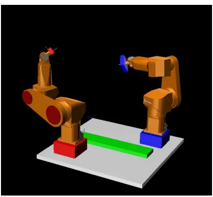
Figure 6: Kinematics inversion example using two St¨aubli Rx90 arms.
The proposed method is to simulate uncertainties in the poses of parts. The principle is to use a Monte Carlo simulation by sampling the values of the parameters of the poses in the workcell from probability distributions over these parameters. Instead of displaying a part in a fixed pose in the graphic scene, the part is displayed, with a given frequency, in the poses obtained by this sampling. If the frequency of sampling is high enough, this will give a good visual perception of the geometric uncertainties in the model of the workcell.
Thisvisualizationof uncertainties allows a more concrete perception of their propagation in a given configura-tion. In particular, it allowsgraphic comparison of two different solutions for a given geometric problem.
6
A kinematics inversion example
In this section we describe how to use our CAD modeler for concrete problems. We present in detail a kinematics inversion problem under geometric uncertainties.
6.1
Problem description
Using two St¨aubli Rx90 robot arms with six revolute joints, we are interested in placing two prismatic parts one against the other. The only constraint is that a face of the first part will be in aFace-On-Facerelationship with a face of the second.
The two arms are modeled as a set of parts attached to each other using probabilistic kinematic links. We assume that the more significant uncertainties are on zero positions of the joints. The two parts are also attached to arms’ end effectors using probabilistic kinematic links. The added constraint we wish to satisfy to solve the problem is represented by a link between the two faces to place in Face-On-Facerelationship. We use for this link three Gaussians on the three constrained parameters tz, rx and ry with zeros as mean values and 0.5 mm,
0.01 rad and 0.01 rad respectively as standard deviations. Figure 6 shows the two arms, while Fig. 7 gives the corresponding kinematic graph.
TABLE-FACE
ARM 1 ARM 2
AXIS 1 2 AXIS 1 1
GRIPPER 1 GRIPPER 2 RED-CUBE BLUE-CUBE
FACE 1 FACE 2
Figure 7: The corresponding kinematic graph.
Figure 8: The solution obtained by the system.
6.2
Results
Figure 8 shows the solution obtained by the system. This solution gives maximal precision for the required
Face-On-Facerelationship because:
1. Right Arm(the less accurate) is coiled to minimize the propagation of the uncertainties on its zero positions.
2. Rotation axes are perpendicular to the common normal of the two faces.
Table 1 summarizes the problem complexity and the system performances for this problem using a PowerPC G3/400 machine.
6.3
Discussion
Integration space dimension 50 Optimization space dimension 12 Number of cycles 1 Number of frames 28 Number of inequality constraints 16 Computation time (seconds) 13
Table 1: Some parameters summarizing the problem complexity and the system performances for this kinematics inversion problem.
Figure 9: A parallelepiped pose and dimensions calibration problem using contact relationships.
7
A calibration example
In this section, we present a calibration problem.
7.1
Problem description
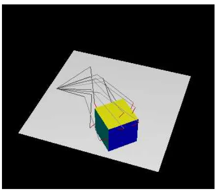
The purpose of this example is to calibrate the pose and the size of a 3-D part. More precisely, we are interested in identifying the parameters of the pose of a parallelepiped on a table and the three dimensions of this parallelepiped (see Fig. 9).
The experimental protocol is as follows. For each measurement, a six DOF arm is moved to a configuration that allows obtaining a contact between a touch sensor mounted on the end effector of the arm and a face of the parallelepiped. A set ofN contacts between the touch sensor and the faces will give the set of N measurements (configurations that allow contact) we will use for calibration (see Fig. 10). The geometric model of the arm is the same used for Lef t Armin the previous example.
We suppose that the parallelepiped lies on the table. Consequently, we have to identify only the x and y
Figure 10: The set of contacts to use for calibration.
Figure 11: Contact points and the parallelepiped faces to put back in contact to solve the calibration problem.
7.2
Results
The a priori distributionp(X) on the search spaceX= (x, y, α, sx, sy, sz)T expresses our prior knowledge on the
parameters to be identified. For this example, we have assumed an uniform distributionp(X) to express the fact that no initial estimation of these parameters is available.
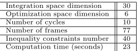
We summarize the problem complexity and the system performances for this problem using a PowerPC G3/400 machine in Tab. 2.
The simulated contacts have been taken at non-null distances between the touch sensor and the parallelepiped faces. Table 3 gives error values for the ten measurements. We have to underline that all these contact errors have positive values because the touch sensor cannot overlap the parallelepiped.
Table 4 gives simulation values of the parameters to calibrate and the values obtained after calibration.
7.3
Discussion
OBJECT
ARM ART 1 1 ART 1 10
END10 END1
TABLE … ..
. .
. .
FACE-UP FACE-FRONT
FACE-DOWN …
Figure 12: The kinematic graph for the calibration problem.
Integration space dimension 30 Optimization space dimension 6
Number of cycles 10
Number of frames 77
Inequality constraints number 40 Computation time (seconds) 23
Table 2: Some parameters summarizing the problem complexity and the system performances for this calibration problem.
• To take into account prior information on the parameters to estimate.
• To take into account, for each measurement (contact), its accuracy by propagating the uncertainties of the arm model. This allows an implicit weighting of these measurements (the more accurate the measurement, the more importance it has in the calibration process).
• To take into account prior information on the used measurement tool. In this particular example where measurements are contact relationships, we have expressed the overlap phenomenon using a non-symmetrical distribution
p(tz) =
2
√
2πσce
−12
t2z σ2
c if tz≥0
0 else
whereσc was 0.5 mm.
8
Conclusion and Future Research
We have presented a generic approach for geometric problem specification and resolution using a Bayesian frame-work. We have shown how a given problem is first represented as a probabilistic kinematic graph and then expressed as an integration/optimization problem. Appropriate numerical algorithms used to apply this method-ology are also described. For generality, no assumptions have been made on the shapes of distributions or on the amplitudes of uncertainties.
Numerous geometric problems have been specified and resolved using our system. We have presented in this paper a kinematics inversion under uncertainties problem and a part pose and shape calibration.
Contact 1 Contact 2 Contact 3 Contact 4 Contact 5
Simulated errors (mm) 0.677 0.567 0.303 0.792 0.724
Contact 6 Contact 7 Contact 8 Contact 9 Contact 10
Simulated errors (mm) 0.791 0.883 0.858 0.383 0.111
Table 3: Error values used when simulating contacts.
x(mm) y(mm) α(rad) sx(mm) sy(mm) sz(mm) Simulation values 900.000 -900.000 0.7854 300.000 300.000 300.000 Calibration results 900.195 -900.000 0.7853 299.238 299.238 299.238
Table 4: Initial values (simulation values) of the parameters to calibrate and calibration results.
For the integration problem, numerical integration can be avoided when the integrand is a product of generalized normals (Dirac delta functions and Gaussians) and when the model is linear or can be linearized (errors are small enough). The optimization algorithm may also be improved by using a local derivative-based method after the convergence of our genetic algorithm.
Future work will aim at allowing the use of high-level sensors such as vision-based ones. We are also considering extending our system so that it can include non-geometrical parameters (inertial parameters for example) in the problem specification.
References
[Alami and Simeon, 1994] Alami, R. and Simeon, T. (1994). Planning robust motion strategies for mobile robots. InProc. of the IEEE Int. Conf. on Robotics and Automation, volume 2, pages 1312–1318, San Diego, California. [Bar-Shalom and Fortmann, 1988] Bar-Shalom, Y. and Fortmann, T. E. (1988). Tracking and Data Association.
Academic Press.
[Bessi`ere et al., 1998] Bessi`ere, P., Dedieu, E., Lebeltel, O., Mazer, E., and Mekhnacha, K. (1998). Interpr´etation ou description (I): Proposition pour une th´eorie probabiliste des syst`emes cognitifs sensori-moteurs.Intellectica, 26-27:257–311.
[Dellaert et al., 1999] Dellaert, F., Fox, D., Burgard, W., and Thrun, S. (1999). Monte Carlo localization for mobile robots. InProc. of the IEEE Int. Conf. on Robotics and Automation, Detroit, MI.
[Geweke, 1996] Geweke, J. (1996). Monte Carlo simulation and numerical integration. In Amman, H., Kendrick, D., and Rust, J., editors, Handbook of Computational Economics, volume 13, pages 731–800. Elsevier North-Holland, Amsterdam.
[Gondran and Minoux, 1990] Gondran, M. and Minoux, M. (1990). Graphes et Algorithmes. Eyrolle, Paris. [Grefenstette, 1988] Grefenstette, J. J. (1988). Credit assignment in rule discovery systems based on genetic
algorithms. Machine Learning, 3:225–245.
[Holland, 1975] Holland, J. H. (1975). Adaptation in Natural and Artificial Systems. University of Michigan Press, Ann Arbor, MI.
[Jaakkola and Jordan, 1999] Jaakkola, T. and Jordan, M. (1999). Variational probabilistic inference and the QMR-DT network. J. Artif. Intellig. Res. (JAIR), 10:291–322.
[Jaynes, 1996] Jaynes, E. T. (1996). Probability Theory - The Logic of Science. Unfinished book publicly available at http://bayes.wustl.edu.
[Keller, 1996] Keller, A. (1996). The fast calculation of form factors using low discrepancy point sequence. In
[Laplace, 1774] Laplace, P. S. (1774). M´emoire sur la probabilit´e de causes par les ´evenements. M´emoire de l’Acad´emie Royale des Sciences, 6:621–656.
[Lozano-P`erez, 1987] Lozano-P`erez, T. (1987). A simple motion-planning algorithm for general robot manipula-tors. IEEE J. of Robotics and Automation, 3(3):224–238.
[Mazer et al., 1998] Mazer, E., Ahuactzin, J., and Bessi`ere, P. (1998). The Ariadne’s Clew algorithm. J. Artif. Intellig. Res. (JAIR), 9:295–316.
[Mekhnacha, 1999] Mekhnacha, K. (1999).M´ethodes probabilistes Bayesiennes pour la prise en compte des incer-titudes g´eom´etriques: application `a la CAO-robotique. Th`ese de doctorat, Inst. Nat. Polytechnique de Grenoble, Grenoble, France.
[Mekhnacha et al., 2000] Mekhnacha, K., Mazer, E., and Bessi`ere, P. (2000). A Bayesian CAD system for robotic applications. InProc. of the IASTED Int. Conf. on Modelling and Simulation, pages 527–534, Pittsburgh, PA, USA.
[Moravec, 1988] Moravec, H. P. (1988). Sensor fusion in certainty grids for mobile robots. AI Magazine, 9(2):61– 74.
[Neal, 1993] Neal, R. M. (1993). Probabilistic inference using Markov Chain Monte Carlo methods. Research Report CRG-TR-93-1, Dept. of Computer Science, University of Toronto.
[Owen, 1996] Owen, J. C. (1996). Constraints on simple geometry in two and three dimensions. Int. J. of Computational Geometry and Applications, 6(4):421–434.
[Presse and Gautier, 1992] Presse, C. and Gautier, M. (1992). Bayesian estimation of inertial parameters of robots. InProc. of the IEEE Int. Conf. on Robotics and Automation, volume 1, pages 364–369, Nice, France. [Puget, 1989] Puget, P. (1989). V´erification-Correction de programme pour la prise en compte des incertitudes en programmation automatique des robots. Th`ese de doctorat, Inst. Nat. Polytechnique de Grenoble, Grenoble, France.
[Sanderson, 1997] Sanderson, A. C. (1997). Assemblability based on maximum likelihood configuration of toler-ances. In Proc. of the IEEE Symposium on Assembly and Task Planning, Marina del Rey, CA.
[Taylor, 1976] Taylor, R. (1976). A synthesis of manipulator control programs from task-level specifications. Ph.d thesis, Stanford University, Computer Science Department.
[Thrun, 1998] Thrun, S. (1998). Bayesian landmark learning for mobile robot localization. Machine Learning, 33(1):41–76.
[Weiss and Adelson, 1998] Weiss, Y. and Adelson, E. H. (1998). Slow and smooth: a Bayesian theory for the combination of local motion signals in human vision. Research Report AI Memo 1624, MIT.