Dynamic Measurements with the Bicone Interfacial
Shear Rheometer: Numerical Bench-Marking of Flow
Field Based Data Processing
Pablo Sánchez-Puga1,‡, Javier Tajuelo Rodríguez1,2,3,†,‡, Juan Manuel Pastor4,‡, and Miguel Ángel Rubio1,‡
1 Dpto. Física Fundamental, Fac. Ciencias, Universidad Nacional de Educación a Distancia (UNED), Senda
del Rey 9, Madrid 28040; [email protected]; [email protected]
2 Dpto. Física Aplicada, Fac. Ciencias, Universidad de Granada, Avenida Fuente Nueva s/n, Granada 18071;
3 Dpt. of Chemichal Engineering, Stanford University, USA
4 Grupo de Sistemas Complejos, ETSIAAB, Universidad Politécnica de Madrid, Av. Puerta de Hierro 4,
Madrid 28040; [email protected]
* Correspondence: [email protected]; Tel.: +34-91-398-7129 † Current address: Affiliation 3
‡ These authors contributed equally to this work.
Version October 8, 2018 submitted to Preprints
Abstract:Flow field based methods are becoming increasingly popular for the analysis of interfacial
1
shear rheology data. Such methods take properly into account the subphase drag by solving the
2
Navier-Stokes equations for the bulk phases flows, together with the Boussinesq-Scriven boundary
3
condition at the fluid-fluid interface, and the probe equation of motion. Such methods have been
4
successfully implemented at the double wall-ring (DWR), the magnetic rod (MR), and the bicone
5
interfacial shear rheometers. However, a study of the errors introduced directly by the numerical
6
processing is still lacking. Here we report on a study of the errors introduced exclusively by the
7
numerical procedure corresponding to the bicone geometry at an air-water interface. In our study we
8
directly input a preset the value of the complex interfacial viscosity and we numerically obtain the
9
corresponding flow field and the complex amplitude ratio for the probe motion. Then we use the
10
standard iterative procedure to obtain the calculated complex viscosity value. A detailed comparison
11
of the set and calculated complex viscosity values is made upon changing different parameters
12
such as real and imaginary parts of the complex interfacial viscosity and frequency. The observed
13
discrepancies yield a detailed landscape of the numerically introduced errors.
14
Keywords:interfacial rheology; interfacial shear rheometer; bicone interfacial rheometer; flow field
15
based data processing.
16
1. Introduction 17
Complex interfacial fluid systems have received much attention in recent years because of their
18
interest from, both, a fundamental and applied point of view in living and industrial systems [1].
19
Systems such as the tear film, the lung’s internal fluid film, cell membranes, foams, and emulsions
20
constitute examples of complex interfacial fluid systems whose dynamical properties play a crucial
21
role regarding their function or utility. Indeed, knowledge of the mechanical properties of such fluid
22
interfacial systems is an essential factor in the development of medical therapies in lung [2] or eye
23
diseases [3], or in the stability and performance of industrial products in the food [4], personal care
24
[5,6], and oil recovery sectors [7].
25
The characterization of the rheology (mechanical properties) of complex interfacial fluid systems
26
is a powerful tool to unravel the physico-chemical phenomena occurring in interfacial processes [1]. A
27
full characterization of the mechanical properties of plane interfacial systems requires studying the
28
mechanical response in two deformation modes[8], namely, shear mode, that keeps the area constant
29
while allowing for shape changes, and dilatational mode, that keeps the shape unchanged while
30
allowing for area changes. In this report we will restrict ourselves to the shear deformation mode.
31
A very convenient way to characterize the dynamical viscoelasticity properties of complex fluid
32
interfaces is through the low amplitude oscillatory motion of a probe located at the interface [9],
33
which allows to describe the interface rheology in terms of a complex interfacial dynamic modulus,
34
G∗s(ω) = Gs0(ω) +iG00s(ω), where Gs0(ω)accounts for the elastic component of the response and is
35
called the interfacial storage modulus, andGs00(ω)represents the viscous component of the response
36
and is called the interfacial loss modulus. Alternatively, a complex interfacial viscosity can be defined
37
asηs∗(ω) =ηs0(ω)−iηs00(ω) =iGs∗(ω)/ω, whose components are related to the interfacial dynamic 38
moduli byηs0 =Gs00/ωandη00s =G0s/ω. 39
Many experimental realizations of such oscillating probe techniques have been proposed and,
40
as of today, three of them emerge as largely popular configurations for Interfacial Shear Rheometers
41
(ISR hereafter). Two of them are built around conventional rotational rheometers by using purposely
42
designed fixtures: a bicone bob [10] or a double wall-ring (DWR hereafter) [11]. The third configuration
43
uses a magnetic rod probe whose oscillation is forced by either a suitably driven Helmholtz coil pair
44
[12] or a mobile magnetic tweezers actuator [13].
45
In all configurations the complex interfacial dynamic moduli or viscosities are obtained through the relationship between the amplitudes of the driving torque (or force) and angular (or linear) displacement, and their phase difference. However, subtracting the effect of the subphase drag on the probe motion is, both, of paramount importance and highly non-trivial. An indication of the relative importance of the interface and subphase drags on the probe is given by the complex Boussinesq number,Bo∗. For instance, in the case of an air/water interfaceBo∗is defined as [14]:
Bo∗= η
∗
s
Lη, (1)
whereηs∗is the complex interfacial viscosity,ηis the subphase bulk viscosity andLis a characteristic 46
length scale that depends on the geometric configuration of the rheometer. The pioneering work in Ref.
47
[15] opened the way to use computed flow fields in the interpretation of the interfacial rheology data. A
48
further step forward was taken by introducing an iterative scheme to recover the value of the complex
49
interfacial viscosity using the computationally obtained flow field and the experimental values of the
50
torque and angle amplitudes and relative phase in the DWR interfacial rheometer [11]. Since then,
51
several flow field based data processing schemes, adequate for the magnetic rod ISR [13,16,17] and the
52
bicone ISR [18], have been proposed to take properly into account the subphase drag on the probe.
53
Such schemes share a common structure, starting from a "seed" value of the complex interfacial
54
viscosity, namely:
55
1. Solve the Navier-Stokes equations for the subphase flow field with no slip boundary conditions at
56
the container and probe walls, and the Boussinesq-Scriven boundary condition at the interface.
57
2. Use the obtained flow field to compute the subphase and interface drags on the probe.
58
3. Use the probe equations of motion to obtain a new prediction for the value of the complex interfacial
59
viscosity.
60
4. Go back to step 1 till convergence is obtained for the value of the complex interfacial viscosity.
61
Such schemes have rendered excellent results in the DWR [11], the magnetic rod ISRs, both in the
62
Helmholtz coil [16] and the magnetic tweezers [13] configurations, and the bicone ISR [18], yielding
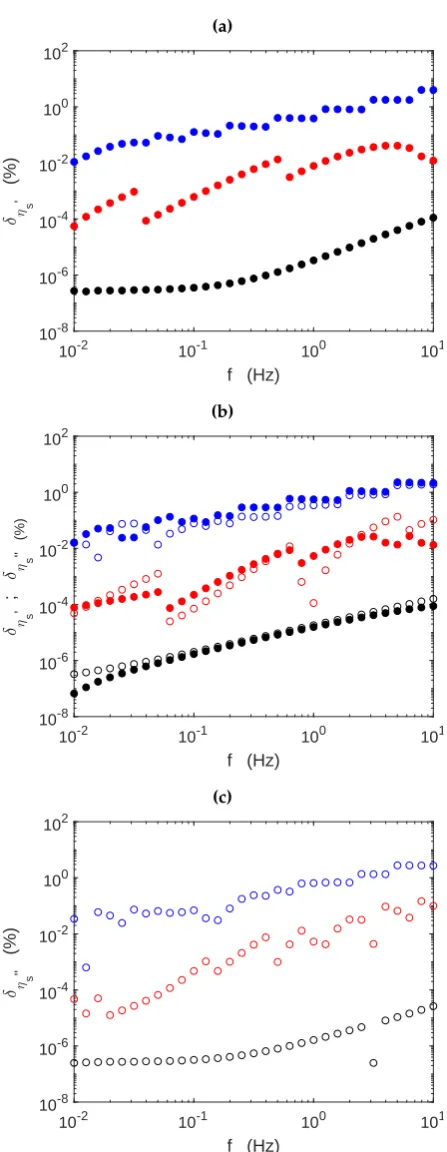
63
good values of the complex interfacial viscosity and providing a more realistic separation of the real
64
and imaginary parts of the complex interfacial viscosity.
65
From a practical point of view, an essential characteristic of each of the above mentioned ISRs is
66
their respective measuring range in a parameter space defined byη0s,ηs00, andω. In this aspect, assessing 67
the performance of the flow field based iterative process is of paramount importance, particularly in
the case of the bicone ISR, due to the comparatively higher role played by the subphase because of
69
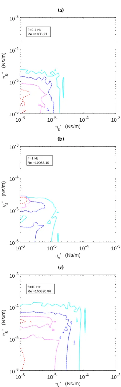
the larger subphase contact with the probe lower surface, that renders comparatively lower values of
70
Bo∗[19]. Limited studies [18,20] of the available measuring range and the errors introduced by the
71
iterative process have been made in the case of the bicone ISR.
72
Here we report on a more complete numerical bench-marking of the flow field based data
73
processing scheme when applied to the bicone ISR. This study has been made using used a software
74
package that we have recently made publicly available [21]. The software package uses an iterative
75
scheme defined directly uponBo∗, and makes extensive use of the sparse matrix functions in MATLAB.
76
In that purpose, we have defined two numerical problems, a direct one -givenηs0,η00s, andω, find 77
the complex amplitude ratio,AR∗- and an inverse one -givenAR∗andωfindηs0andη00s through the 78
iterative process-. The software has been slightly modified so that the the flow field obtained with
79
the "seed"ηs0andηs00values is used to obtain the complex amplitude ratio which is the solution of the 80
direct problem.
81
Using the output of the direct problem as input of the inverse one, we have made a detailed
82
study of the consistency of the iterative data processing scheme in terms of the differences appearing
83
between the complex viscosity input values of the direct problem and the corresponding output values
84
of the inverse problem. Further imposing the requirement that the complex amplitude ratio must be
85
different from the one corresponding to a clean water interface allows us to draw a complete map
86
of the parameter space available to the bicone ISR when using the flow field based data processing
87
scheme.
88
2. Results 89
In this section we show the results obtained through extensive numerical calculations aiming at
90
evaluating the performance of the iterative data processing scheme when applied to a bicone interfacial
91
rheometer working in oscillatory mode at an air/water interface.
92
A careful evaluation of the dependence on the mesh size of the spatial velocity gradients
93
representation, the number of iterations needed for convergence, and the computational costs of
94
the procedure was reported in Ref. [20], where preliminary explorations of the consistency of the
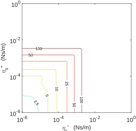
95
iterative data processing scheme, by sweeping in the complex interfacial viscosity while keepingω 96
constant were also included.
97
Here we will focus, first, on checking the consistency of the iterative processing scheme upon
98
changes of the oscillation frequency in the typical range explored in real experiments, and, second,
99
on analyzing the measuring range achievable with a bicone ISR when using the proposed flow field
100
based data analysis scheme. This last aspect will be illustrated through the analysis of the achievable
101
measuring range of a bicone fixture in our Bohlin C-VOR rheometer.
102
2.1. Consistency of the iterative data analysis scheme
103
2.1.1. Consistency over frequency range
104
We have studied the consistency of the iterative data analysis scheme through the following
105
general procedure: i) Preset the frequency, f, and the complex interfacial viscosity,η∗s progand solve 106
the direct problem that yields the complex amplitude ratioAR∗prog, and ii) use the obtained value of
107
the complex amplitude ratio as input of the inverse problem and obtain the calculated value of the
108
(a)
10-2 10-1 100 101
f (Hz) 10-12
10-10 10-8 10-6 10-4 10-2 100
| s
'|, |
s
''| (Ns/m)
(b)
10-2 10-1 100 101
f (Hz) 0
5 10 15 20 25
iterations
(c)
10-2 10-1 100 101
f (Hz) 10-12
10-10 10-8 10-6 10-4 10-2 100
| s
'|, |
s
''| (Ns/m)
(d)
10-2 10-1 100 101
f (Hz) 0
5 10 15 20 25
iterations
(e)
10-2 10-1 100 101
f (Hz) 10-12
10-10 10-8 10-6 10-4 10-2 100
| s
'|, |
s
''| (Ns/m)
(f)
10-2 10-1 100 101
f (Hz) 0
5 10 15 20 25
iterations
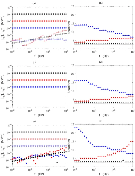
In Fig.1we show the results of such a procedure for a frequency sweep in the range 10−2≤ f ≤10
110
Hz. Representative values of the complex interfacial viscosity have been chosen, namely, a purely
111
viscous interface (ηs∗=η0s, i.e.,η00s =0), a viscoelastic interface (η∗s =ηs0−iηs00, whereη0s =ηs00), and a 112
purely elastic interface (η∗s =−iηs0, i.e.,η0 =0). Three typical numerical values ofηshave been used in
113
the above described cases:ηs=10−6,ηs =10−4,ηs =10−2, in units of N s/m.
114
The graphs on the left column illustrate the results obtained forηscalc0 andη00s calcas a function of 115
frequency, while the right column holds the graphs of the number of iterations needed for convergence
116
at each frequency. The graphs at the upper row (graphs (a) and (b)) pertain to the purely viscous
117
interface, those at the middle row (graphs (c) and (d)) to the viscoelastic interface, and the lower row
118
graphs ((e) and (f)) show the data corresponding to the purely elastic interface. In the left column
119
graphs, filled and empty circles are used to represent the values ofηscalc0 andηs calc00 , respectively. 120
Symbol’s colours black, red, and blue correspond, respectively, to the high, middle, and low numerical
121
values ofηsmentioned above.
122
The agreement between the obtained viscosity component values and the non null programmed
123
values is remarkable (in the case of the viscoelastic interface solid and empty circles superpose as
124
expected). However, unavoidable numerical errors and the finite convergence tolerance, given by
125
thetol Minparameter (Eq.10), necessarily give rise to non null values ofη00s calcfor the purely viscous 126
interface (graphs (a) and (b)) andη0scalcfor the purely elastic interface (graphs (e) and (f)). Fortunately, 127
these pathological non null values are in all of the cases here studied more than two orders of magnitude
128
below their measurable counterparts (η0scalcfor the purely viscous interface andηs calc00 for the purely 129
elastic interface).
130
The graphs on the right column show that in the studied frequency range, convergence in the
131
inverse problem always occurs in less than 25 iterations. Particularly remarkable is the case with the
132
higher complex viscosity modulus (ηs=10−2N s/m, black symbols), where convergence occurs in
133
three iterations for the whole frequency range. Interestingly, for intermediate values of the complex
134
viscosity modulus (red symbols) increasing the frequency has a destabilizing effect (more iterations
135
are required for convergence), while for very low complex viscosity modulus (blue symbols) the effect
136
is just the opposite (less iterations are needed for convergence upon increasing the frequency).
137
The visual agreement between the obtained viscosity component values and the non null
138
programmed values in the graphs on the left column of Fig.1can be better ascertained calculating the
139
relative difference between the programmed and calculated values and representing it in a logarithmic
140
vertical scale. Fig.2shows such graphs, where row arrangement and symbols’ shapes and colours
141
maintain the same codding as in Fig.1. To be specific, the relative differences have been calculated as:
142
δη0=100×
η0scalc−ηs prog0 η0s prog
; δη00 =100×
ηs calc00 −ηs prog00 ηs prog00
Several common features appear in the three graphs included in Fig. 2. First, the relative
143
differences are overall increasing functions of frequency, although non monotonic in some cases.
144
Second, the relative differences are higher the smaller the value ofηs0orη00s. Nonetheless, such relative
145
differences are of the order of a few percent in the worst case -lowest numerical value ofη0sorη00s and 146
highest frequency value- and smaller in all of the other cases. In the case of the viscoelastic interface
147
the relative differences are very similar in, both, the real and imaginary parts of the complex viscosity.
(a)
10-2 10-1 100 101
f (Hz)
10-8 10-6 10-4 10-2 100 102
s
'
(%)
(b)
10-2 10-1 100 101
f (Hz)
10-8 10-6 10-4 10-2 100 102
s
'
;
s
'' (%)
(c)
10-2 10-1 100 101
f (Hz)
10-8 10-6 10-4 10-2 100 102
s
''
(%)
2.1.2. Consistency in the complex plane
149
A complementary view of the consistency problem can be drawn through the percentage modulus
150
of the complex relative differences betweenη∗s calcandη∗s prog, i.e., 151
δmod =100×
ηs prog∗ −ηs calc∗ η∗s prog
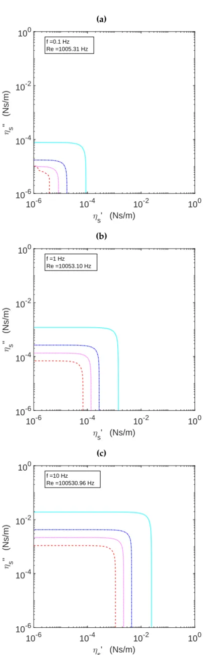
We have calculated the values ofδmodat 60×60 logarithmically spaced points in the (ηs0,η00s) 152
plane, in the range 10−6≤ηs0,ηs00≤10−3in units of N s/m, at three representative frequency values,
153
namely, 0.1, 1, and 10 Hz. The values so obtained have been used to construct contour plots ofδmodin
154
the(ηs0,ηs00)plane, which are shown in Fig.3. The contour lines correspond to the percentage values of 155
δmodindicated in the caption.
(a)
10-6 10-5 10-4 10-3
s' (Ns/m)
10-6 10-5 10-4 10-3
s
'' (Ns/m)
f =0.1 Hz Re =1005.31
(b)
10-6 10-5 10-4 10-3
s' (Ns/m)
10-6 10-5 10-4 10-3
s
'' (Ns/m)
f =1 Hz Re =10053.10
(c)
10-6 10-5 10-4 10-3
s' (Ns/m)
10-6 10-5 10-4 10-3
s
'' (Ns/m)
f =10 Hz Re =100530.96
The aspect of the contour lines is not smooth, with even the appearance of some islands. However,
157
it might be possible that such islands are an artifact caused by the limited resolution of only 60×60
158
points in the(ηs0,ηs00)plane, due to the high computational cost of these simulations. 159
However, some general observations can be done on Fig.3. In the three cases here considered, the
160
structure of the contour lines corresponding to the lower values ofδmod(continuous light blue lines) is
161
roughly square, while strong peaks (red dashed lines) appear close to the lower values ofη0s, i.e., in 162
elasticity dominated interfaces.
163
Regarding the performance of the iterative data processing scheme it is important to look at the
164
numerical values ofδmodin each of the graphs having in mind that it represents the modulus of the
165
relative difference between two values of the complex interfacial viscosity: the programmed value at
166
the start of the direct problem and the calculated value at the end of the inverse problem.
167
In the (a) graphδmodtakes very low values all of them being lower than 0.2%, whileδmod ≤0.1% 168
in the region such thatη0s≥2×10⁻⁶andηs00≥10−5in units of N m/s. This means that the iterative
169
process introduces very small errors (≤0.1%) in the interfacial viscosity measurements within most of
170
the(ηs0,ηs00)range here considered provided they are made at low oscillation frequencies (0.1 Hz in the 171
top graph).
172
In the (b) graph of Fig. 3the values ofδmod are much higher (up to 60% at the peak), while
173
δmod≤0.15% in the region such thatηs0 ≥10−5andη00s ≥3×10⁻⁵. Hence, the(ηs0,η00s)range in which 174
the iterative process introduces small errors decreases significantly at an oscillations frequency of 1 Hz.
175
This tendency is again clear in graph (c) of Fig.3. Although the values ofδmodare lower than in
176
the previous case (about 2.5% at the peak), the low error region (δmod≤0.2%) shrinks again to values
177
such thatηs0 ≥10−4andη00s ≥10−4in units of N m/s. 178
2.2. Estimation of the achievable measuring range
179
To elucidate which is the achievable measuring range of a bicone ISR when using the proposed
180
flow field based data analysis scheme two main aspects have to be considered. On the one hand the
181
instrumental errors, i.e., the unavoidable dispersion in the torque and angular displacement data
182
measured by the rheometer. On the other hand the rheometry point of view, i.e., the fact that for
183
the measurements to be acceptable they must be distinguishable from those pertaining to a clean
184
water interface. The interplay between these two aspects is illustrated here through the analysis of the
185
achievable measuring range of a bicone fixture in a Bohlin C-VOR rheometer.
186
In oscillatory measurements, the output of the rheometer comprises the amplitudes of the torque
187
and the angular displacement, and their relative phase, which are used to determine the experimental
188
value of the amplitude ratio, AR∗exp. Given a surfactant laden interface, the instrument can resolve
189
its complex viscosity if the corresponding complex amplitude ratio can be distinguished from that
190
pertaining to a clean water interface. In Ref. [18] this condition was formally expressed as two
191
inequalities that, both, had to be fulfilled simultaneously.
192
AR
∗
exp
− |AR
∗
clean|
≥σ(|AR
∗clean|); arg(AR
∗
exp)−arg(AR∗clean)
≥σ(arg(AR ∗
clean)). (2) In order to apply Eqs.2we have calculated bothAR∗expandARclean∗ for differentη0s,ηs00combinations 193
(all the combinations of 120 values logarithmically spaced in each axis) and different frequencies.
194
The corresponding values for the uncertainties σ(AR∗clean
) and σ(arg(AR∗clean) were taken from 195
experiments performed on clean water interfaces at the Bohlin C-VOR rheometer.
196
In Fig. 4(a) we show the lines satisfying the equality in Eq. 2, i.e., the lower resolvable limit,
197
for frequencies in the range 0.1≤ f ≤ 100 Hz. For a clearer view, the lines corresponding to three
198
representative frequencies, namely, f =0.1, 1, and 10 Hz, are shown in Fig.4(b).
199
The structure of the non-measurable region has some common features at all frequencies, such
200
as the spiky tongue that widens at lower values of the real and imaginary parts of the viscosity. The
island like structures at the tips of the tongues are artifacts caused by the width of the tongue being
202
comparable to the distance between sampled points in the(ηs0,ηs00)plane. In fact such islands should 203
actually correspond to points corresponding to a continuous tongue that is getting thinner and thinner.
204
The tongues shift to cover larger values ofηs0andηs00as the frequency increases. 205
For viscosity dominated interfaces (very low η00s) there is, at each frequency, a well defined
206
threshold interfacial viscosity below which the interface is non-distinguishable from a clean water
207
interface. Roughly speaking those thresholds are (in N s/m units) 2×10⁻⁶for f =0.1 Hz, 3×10⁻⁵
208
forf =1 Hz, and 3×10⁻³for f =10Hz. This behavior coincides with the results shown in Fig. 7.c of
209
Ref. [18].
210
A different behavior is seen for viscoelastic interfaces. Let’s consider viscoelastic interfaces with
211
ηs0 =ηs00(points a the bisectrix of Fig.4either (a) or (b)). For low values ofηs, the points lay in the base 212
of the tongue and, therefore, the interface is non-distinguishable from a clean water one. Increasing
213
inηs0 =ηs00the tongue crosses below the bisectrix and, therefore, the points at the bisectrix become
214
distinguishable from a clean water interfaces. Upon further increasingηs0 = ηs00the tongue turns 215
up and crosses again the bisectrix in a region in which the tongue is already very narrow. Hence, a
216
very narrow window appears in which the interface is again non-distinguishable from a clean water
217
one. Forηs0 = η00s values larger than those at the above mentioned window the interface is again
218
distinguishable from clean water. This behavior coincides with the results shown in Fig. 7.b of Ref.
219
[18].
220
For elasticity dominated interfaces (η00s η0s) one finds (see lines corresponding tof =0.1 and
221
1 Hz) that at low values ofηs00the interface is not distinguishable from a clean water one, and there 222
is, at each frequency, a well defined threshold interfacial elastic component (ηs00) below which the 223
interface is non-distinguishable from a clean water interface. Above the threshold value the interfacial
224
viscoelasticity can be measured. This scenario coincides with the results shown in Figs. 4c and 4e
225
of the Supporting information of Ref. [18] except that in those figures narrow tongues in which the
226
interface is again non-distinguishable from a clean water one. This means that the sampling of the
227
(ηs0,ηs00) plane in Fig.4is not enough to fully represent the narrow parts of the tongues. 228
All of the above mentioned features come from the non-fulfillment of the condition on the moduli.
229
At large frequencies, however, the non-fulfillment of the condition on the arguments in Eq.2causes
230
an additional enlargement of the non-distinguishable region in elasticity dominated interfaces. For
231
instance, the line corresponding to f =10 Hz in Fig. 4(b) shows a bump at high values ofη00s and 232
comparatively lower values ofη0s. Actually, in our numerical simulations that bump appears at all
233
frequency values above 2.5 Hz, and shifts upwards and rightwards upon increasing the frequency (see
234
Fig.4(a)). Indeed, as from our simulations, it cannot be discarded that for lower frequencies similar
235
bumps appears too although at valuesηs0 ≤10−6N s/m.
(a)
10-6 10-4 10-2 100
s' (Ns/m)
10-6 10-4 10-2 100
s
'' (Ns/m)
0.1
0.25
0.25 0.5
0.5
1
1
1
2.5
2.5 5
5 10
10 25
25 50
50
50
100
100
100
(b)
10
10-6 10-4 10-2 100
s' (Ns/m)
10-6 10-4 10-2 100
s
'' (Ns/m)
Figure 4. Boundaries separating the regions of the (η0s,η00s) plane where the interface can be distinguished from a clean air-water interface, under fulfillment of both conditions in Eq. 2. (a) Lines at frequencies indicated by the line labels in the frequency range 0.1≤ f ≤100 Hz. (b) Lines at representative frequencies: f =0.1 Hz (black continuous line), f =1 Hz (blue dash-dot line), and
f=10 Hz (red dotted line).
The distinguishability criterion based on simultaneous fulfillment of the two inequalities in Eq.2 237
is, however, somewhat too strict. In fact, when any of the two inequalities is fulfilled the interface is
238
already distinguishable from the clean water interface. If we use this relaxed criterion with the output
239
of our simulations the picture so obtained is shown in Fig.5, where both the resonance tongues, due to
240
the condition on the moduli, and the bumps at the elasticity dominated region, due to the condition on
241
the arguments, have disappeared.
242
10-6 10-4 10-2 100
s' (Ns/m)
10-6 10-4 10-2 100
s
'' (Ns/m)
2.5 5
10
25
50
50
100
100
2.3. Global relative errors
243
In the previous subsections we have illustrated separately the errors introduced by the iterative
244
process and the regions where interface can be distinguished from a clean water one. However, in actual
245
experiments these two effects are coupled, because what one has as the result of an experiment is the
246
values of the modulus and argument of the complex amplitude ratio,
AR
∗
exp
andδexp =arg(AR ∗
exp),
247
each one of then affected by its own experimental uncertainty,σ AR ∗ exp andσ
arg(AR∗exp)
. So,
248
the problem here is how the small area around the experimental values defined by the rectangle defined
249
by the points
AR ∗ exp ±σ AR ∗ exp
,δexp±σ
arg(AR∗exp)
transforms under the application of
250
the iterative procedure.
251
In order to estimate that transformation, we program 60×60 η0s prog and ηs prog00 values in a
logarithmic mesh in theη0s prog,η00s prog
, and use them as input values for the direct problem, having as output the values of
AR
∗
prog
andδprog. For each of those data we use as uncertainty the experimental
uncertainty measured for a clean water interface at the corresponding frequency, and define an enclosing rectangle with the points
AR ∗ prog ±σ AR∗clean
,δprog±σ arg(AR∗clean)
. Next we use the corners of such a rectangle plus the middle points of the four rectangle faces as input of the inverse problem. Then, for each point in the plane
AR
∗
prog
,δprog
we now have eight images in the plane
(η0siter,ηs iter00 ), that we labelη∗sirect; i=1, ..., 8, corresponding to the pertaining eight points that define
the corresponding rectangle given by experimental uncertainties. Now, we define as a global error indicator,e(ηs prog∗ ), the maximal percentage relative difference between the programmed value of the
complex interfacial viscosity,ηs prog∗ , and the eight pointsη∗sirect, i.e.,
e(ηs prog∗ ) =100×max (
η∗s prog−ηs rect∗ i ηs prog∗
) , (3)
The results of the application of such a procedure are shown en Fig.6, for three representative
252
frequencies, namely, f =0.1 Hz, f =1 Hz, and f =10 Hz. In all of the three graphs, the contour lines,
253
from right to left and top to bottom, correspond to the valuese(ηs prog∗ ) =1, 5, 10, 20 %. 254
Loosely speaking, if we take the 5% line as an acceptable error, the bicone fixture mounted in
255
a Bohlin C-VOR rheometer with the flow field data processing scheme described in Ref. [18] can be
256
expected to accurately measure complex interfacial viscosities (in Ns/m units) down to 2×10⁻⁵, for
257
f =0.1 Hz, 3×10⁻⁴, for f =1 Hz, and 4×10⁻³, for f =10 Hz.
(a)
10-6 10-4 10-2 100
s' (Ns/m)
10-6 10-4 10-2 100
s
'' (Ns/m)
f =0.1 Hz Re =1005.31 Hz
(b)
10-6 10-4 10-2 100
s' (Ns/m)
10-6 10-4 10-2 100
s
'' (Ns/m)
f =1 Hz Re =10053.10 Hz
(c)
10-6 10-4 10-2 100
s' (Ns/m)
10-6 10-4 10-2 100
s
'' (Ns/m)
f =10 Hz Re =100530.96 Hz
Figure 6. Contour plots ofe(ηs prog∗ )in the(ηs0,ηs00)plane at the frequency value indicated in the
corresponding legend. The contour lines correspond to the following percentage values ofe(ηs prog∗ ),
3. Discussion 259
Apart from the comments already made while describing the results, several general questions
260
deserve further discussion. First of all, why the solutions to the direct and the inverse problems may
261
differ? In our opinion, the answer is that the direct and the inverse problems do not correspond to
262
the same type of experiment. On the one hand, in the direct problem, the angular displacement of the
263
probe is prescribed, which means the strain is prescribed and the probe equation of motion is used
264
merely to obtain the corresponding complex amplitude ratio, i.e., the torque, which is directly related
265
to the shear stress. In this sense the direct problem appears to be a strain controlled experiment.
266
On the other hand, in the inverse problem the complex amplitude ratio is prescribed and
267
the iterative process yields the value of the complex interfacial viscosity and the complex velocity
268
amplitude function that are compatible with the prescribed complex amplitude ratio. At each step of
269
the iterative process, rotor inertia is taken into account, and, more importantly, changes in the complex
270
velocity amplitude involve changes in the subphase and interface drag terms in Eq.9. Therefore, the
271
inverse problem appears to correspond closely to a stress controlled experiment. Hence, it is not so
272
surprising that the solutions of the direct and inverse problems might differ somewhat.
273
Another aspect that deserves a comment is the remarkable frequency dependence of the peak
274
values ofδmodin Fig.3, and which might be its origin. At low frequency values, fluid and rotor inertia
275
do not play any role, and the velocity profile at the subphase and interface is linear. Hence, both the
276
direct and the inverse problems have to give solutions very close to the linear velocity profile solution
277
[18] and, therefore, the relative difference between their results must be small. At large frequency
278
values, rotor inertia (theIω2term in Eqs. 8and9) dominates the dynamics, and the subphase and 279
the interface do not play a leading role. Hence, the solutions of the direct and inverse problems must
280
be again very similar, so that the values of the relative difference must be small here too. On the
281
contrary, at intermediate frequency values, fluid inertia plays an essential role, the velocity profiles
282
being strongly nonlinear and, more importantly, the inverse problem allows for variations in the
283
velocity profileg∗(r, ¯¯ z)as iterations proceed, which may strongly affect the converged value ofBo∗
284
and, hence, the value ofηs calc∗ . 285
When resonance phenomena [18,20] appear large amplitudes, nonlinear behavior, and instabilities
286
may occur. It is important to realize that the ansatz (Eq.4) and the hydrodynamic model described
287
in Section 4 allow us to obtain periodic fulfilling the ansatz. However, it is not guaranteed that such
288
solutions are the only ones possible, neither that they are stable. Fully dynamical simulations of the
289
probe equation of motion coupled to the hydrodynamic model should shed light on other possibly
290
existing solutions and their stability.
291
4. Materials and Methods 292
4.1. Hydrodynamic model and data analysis scheme
293
The hydrodynamic model and data analysis scheme have been fully described elsewhere [20]. We
294
reproduce it here just for the sake of completeness.
295
The interface is considered flat and horizontal, and the flow, both at the subphase and the interfaces is considered horizontal and axially symmetric. The angular oscillation of the bicone is considered periodic, with frequencyω. Hence, the bicone angular oscillation and the velocity at the
bicone rim can be written as:
θ(t) =θ0eiωt; vθ(Rb,h,t) =i Rbωθ0e
iωt.
Under such approximations the spatial dependence of the fluid velocity field can be represented by a complex amplitude functiong∗(r,z)so that
where the spatial variables have been made non-dimensional takingRbas characteristic length scale.
296
The complex amplitude function must obey Eq.5, derived from the Navier-Stokes equations, which in
297
non-dimensional form read
298
i Re∗g∗(r, ¯¯ z) = ∂
2g∗(r, ¯¯ z) ∂r¯2 +
∂2g∗(r, ¯¯ z) ∂z¯2 +
1 ¯ r
∂g∗(r, ¯¯ z)
∂r¯ −
g∗(r, ¯¯ z)
¯
r2 , (5)
whereRe∗is the Reynolds number,Re∗=ρωR2c/η∗(possibly complex if the bulk subphase viscosity 299
is complex). The boundary conditions are no-slip at the cup and bicone bob walls (Eq. 6) and the
300
Boussinesq-Scriven boundary condition (tangential stress balance) at the interface (Eq.7) are
301
g∗(r, 0¯ ) =g∗(1, ¯z) =0, g∗(0, ¯z) =0,
g∗(r¯≤R¯b, ¯h) = r¯
¯ Rb
,
(6)
∂g∗ ∂z¯ =Bo
∗ ∂ ∂r¯
1 ¯ r
∂ ∂r¯(r g¯
∗
)
, at ¯Rb <r¯<1, ¯z=h,¯ (7) whereBo∗=η∗s/Rcη∗.
302
The torque balance equation for the ISR rotor yields Eq.8, that relates the complex amplitude
303
ratio to, both, the Boussinesq number and, implicitly, the velocity amplitude functiong∗(r, ¯¯ z):
304
AR∗=iω2πRbη∗
Z Rb
0 r
2
∂g∗ ∂z
z=h
dr−RbRcBo∗
Rb
∂g∗ ∂r
r=Rb,z=h
−1
−Iω2. (8)
Solving for the Boussinesq number allows one to set up a simple iterative procedure, namely,
305
Bo∗{i+1}=
−AR∗exp−Iω2+iω2πRbη∗
RRb
0 r2
∂g∗{i}
∂z
z=hdr
iω2πη∗R2bRc
Rb ∂g∂∗{ri} r=R
b,z=h
−1
, (9)
whereAR∗exprepresents the complex value of the experimentally obtained amplitude ratio. As the
306
value ofAR∗expcomes directly from the experiments, it seems adequate to establish the convergence
307
upon the complex amplitude ratio as:
308
(AR∗pp)
{i}
calc−(AR
∗
pp)exp
(AR∗
pp)exp
≤tol Min. (10)
4.2. Parameters for the numerical calculations
309
In the present report we have used the geometrical parameters corresponding to the experimental
310
setup of Ref. [18]. Accordingly, we use a cup with radiusRc=0.04 m, and a single-cone bob with a
311
radiusRb =0.034 m and vertical distance to the cup bottomh=0.022 m. The water subphase physical
312
parameters used wereρb =1000 kg m−3andηb=10−3Pa s.
313
For the dynamical parameters of the rheometer we used the measured values [18] corresponding
314
to the Bohlin C-VOR rheometer at our lab, namely, the moment of inertia of the rotor + bicone assembly,
315
I= (2.42±0.02)×10−5kg m2, and the coefficient of the frictional torque of the rheometer (C-VOR,
316
Bohlin Instruments),b= (3.2±0.5)×10−8N m s.
317
Eq. 5was solved with a mesh havingN = 480 sub-intervals in the radiate coordinate, ¯r, and
318
M=240 sub-intervals in the vertical coordinate ¯z. The value of the tolerance parameter used in Eq.
10to define convergence of the iterative process wastol Min=10 , and the maximum number of
320
iterations allowed was 100. According to the results in [20] such values yielded good resolution of the
321
spatial velocity gradients and reasonable convergence times.
322
4.3. Definition of the direct and inverse numerical problems
323
The direct problem merely consists in finding the value of the complex amplitude ratio that
324
corresponds to the programmed values of the frequency,ω, and the complex interfacial viscosity, 325
ηs prog∗ . Hence, it suffices to calculate the corresponding values of the complex Reynolds and Boussinesq 326
numbers, respectively,Re∗progandBo∗prog, and to solve Eq.5with the boundary conditions specified by
327
Eqs.6and7. Then the numerically obtained complex velocity amplitude function,g∗prog(r, ¯¯ z)is used
328
to calculate the value of the complex amplitude ratio,AR∗prog(ω,ηs prog∗ ).
329
Conversely, the inverse problem starts from the numerically obtained values of the complex
330
amplitude ratio,AR∗prog(ω,ηs prog∗ ), and a suitable seed value ofBo∗, that is obtained using a linear 331
approximation in which the complex velocity amplitude function,g∗clean(r, ¯¯ z), corresponding to a clean
332
interface is used as a first approximation (see Ref. [20] for details). Then Eq.9is used to obtain a new
333
calculated value of the Boussinesq number,Bo∗calcand this new value of the Boussinesq number is
334
re-injected into the Boussinesq-Scriven boundary condition, Eq.7. Solving the hydrodynamic problem
335
again (Eqs.5,6, and7) a new flow field configuration (a new complex velocity amplitude function) is
336
obtained which allows us to compute an iterated value of the complex amplitude ratio through Eq.8.
337
This procedure is repeated until convergence according to condition Eq.10occurs. Then Eq.9is used
338
to obtain a converged value of the complex Boussinesq number,Bo∗calc, and a converged value of the
339
complex interfacial viscosity just using the expressionη∗s calc=Rcη∗Bo∗calc. Throughout this work we 340
have used a convergence tolerance oftol Min=10−5.
341
The comparison of the complex viscosity values set at the start of the direct problem with
342
the values obtained from the final solution of the inverse problem gives us a way to evaluate the
343
performance of the iterative data processing scheme.
344
Author Contributions:All authors have contributed equally to this work. 345
Funding:This research was funded by Ministerio de Economía, Industria y Competitividad, Gobierno de España 346
grant numbers FIS2013-47350-C5-5-R and FIS2017-86007-C3-3-P. P.S.P. was funded by Consejería de Educación, 347
Juventud y Deporte, Comunidad de Madrid, Research Assistant grant number PEJ16/IND/AI-1253. 348
Acknowledgments: The authors acknowledge the administrative and technical support provided by M.J. 349
Retuerce. 350
Conflicts of Interest:The authors declare no conflict of interest. The founding sponsors had no role in the design 351
of the study. 352
Abbreviations 353
The following abbreviations are used in this manuscript: 354
355
ISR Interfacial Shear Rheometer DWR Double wall-ring
356
References 357
1. Fuller, G.G.; Vermant, J. Complex Fluid-Fluid Interfaces: Rheology and Structure. Annual Review of Chemical 358
and Biomolecular Engineering2012,3, 519–543. doi:10.1146/annurev-chembioeng-061010-114202. 359
2. Stetten, A.Z.; Iasella, S.V.; Corcoran, T.E.; Garoff, S.; Przybycien, T.M.; Tilton, R.D. Current Opinion in 360
Colloid & Interface Science Surfactant-induced Marangoni transport of lipids and therapeutics within the 361
lung.Current Opinion in Colloid & Interface Science2018,36, 58–69. doi:10.1016/j.cocis.2018.01.001. 362
3. Ezuddin, N.S.; Alawa, K.A.; Galor, A. Therapeutic Strategies to Treat Dry Eye in an Aging Population. Drugs 363
4. Yang, N.; Lv, R.; Jia, J.; Nishinari, K.; Fang, Y. Application of Microrheology in Food Science. Annual Review 365
of Food Science and Technology2017,8, 493–521. doi:10.1146/annurev-food-030216-025859. 366
5. Sharipova, A.; Aidarova, S.; Mutaliyeva, B.; Babayev, A.; Issakhov, M.; Issayeva, A.; Madybekova, G.; 367
Grigoriev, D.; Miller, R. The Use of Polymer and Surfactants for the Microencapsulation and Emulsion 368
Stabilization.Colloids and Interfaces2017,1, 3. doi:10.3390/colloids1010003. 369
6. Berton-Carabin, C.C.; Sagis, L.; Schroën, K. Formation, Structure, and Functionality of Interfacial 370
Layers in Food Emulsions. Annual Review of Food Science and Technology 2018, 9, 551–587. 371
doi:10.1146/annurev-food-030117-012405. 372
7. Langevin, D.; Argillier, J.f. Interfacial behavior of asphaltenes. Advances in Colloid and Interface Science2016, 373
233, 83–93. doi:10.1016/j.cis.2015.10.005. 374
8. Erni, P. Deformation modes of complex fluid interfaces. Soft Matter 2011, 7, 7586–7600. 375
doi:10.1039/c1sm05263b. 376
9. Liggieri, R.; Miller, L.Interfacial Rheology; Brill, 2009. doi:10.1163/ej.9789004175860.i-684. 377
10. Erni, P.; Fischer, P.; Windhab, E.J.; Kusnezov, V.; Stettin, H.; Läuger, J. Stress- and strain-controlled 378
measurements of interfacial shear viscosity and viscoelasticity at liquid/liquid and gas/liquid interfaces. 379
Review of Scientific Instruments2003,74, 4916–4924. doi:10.1063/1.1614433. 380
11. Vandebril, S.; Franck, A.; Fuller, G.G.; Moldenaers, P.; Vermant, J. A double wall-ring geometry for interfacial 381
shear rheometry. Rheologica Acta2010,49, 131–144. doi:10.1007/s00397-009-0407-3. 382
12. Brooks, C.F.; Fuller, G.G.; Frank, C.W.; Robertson, C.R. Interfacial stress rheometer to study rheological 383
transitions in monolayers at the air-water interface. Langmuir1999,15, 2450–2459. doi:10.1021/la980465r. 384
13. Tajuelo, J.; Pastor, J.M.; Rubio, M.A. A magnetic rod interfacial shear rheometer driven by a mobile magnetic 385
trap. Journal of Rheology2016,60, 1095–1113. doi:10.1122/1.4958668. 386
14. Edwards, D.A.; Brenner, H.; Wasan, D.T. Interfacial Transport Processeses and Rheology; 387
Butterworth-Heinemann: Boston, 1991. 388
15. Reynaert, S.; Brooks, C.F.; Moldenaers, P.; Vermant, J.; Fuller, G.G. Analysis of the magnetic rod interfacial 389
stress rheometer. Journal of Rheology2008,52, 261–285. doi:10.1122/1.2798238. 390
16. Verwijlen, T.; Imperiali, L.; Vermant, J. Separating viscoelastic and compressibility contributions in 391
pressure-area isotherm measurements. Advances in Colloid and Interface Science 2014, 206, 428–436. 392
doi:10.1016/j.cis.2013.09.005. 393
17. Tajuelo, J.; Pastor, J.M.; Martínez-Pedrero, F.; Vázquez, M.; Ortega, F.; Rubio, R.G.; Rubio, M.A. Magnetic 394
microwire probes for the magnetic rod interfacial stress rheometer. Langmuir 2015, 31, 1410–1420. 395
doi:10.1021/la5038316. 396
18. Tajuelo, J.; Rubio, M.A.; Pastor, J.M. Flow field based data processing for the oscillating conical bob interfacial 397
shear rheometer. Journal of Rheology2018,62, 295–311. doi:10.1122/1.5012764. 398
19. Guzmán, E.; Tajuelo, J.; Pastor, J.M.; Rubio, M.A.; Ortega, F.; Rubio, R.G. Shear rheology of fluid interfaces: 399
Closing the gap between macro- and micro-rheology. Current Opinion in Colloid & Interface Science2018, 400
37, 33–48. doi:10.1016/j.cocis.2018.05.004. 401
20. Sánchez-Puga, P.; Tajuelo, J.; Pastor, J.M.; Rubio, M.A. BiconeDrag - A data processing application for the 402
oscillating conical bob interfacial shear rheometer,arXiv:1810.01696 403
21. Sanchez-Puga, P.; Tajuelo, J.; Pastor, J.M.; Rubio, M.A. BiconeDrag - A data processing application for the 404