Realization of Maxwell’s Hypothesis An Experiment of Heat-Electric Conversion in Contradiction to the Kelvin Statement

Realization of Maxwell’s Hypothesis

An Experiment of Heat-Electric Conversion

in Contradiction to the Kelvin Statement

Xinyong Fu & Zitao Fu

Shanghai Jiao Tong University July 29, 2020

[email protected] [email protected] Key Words

Maxwell’s demon magnetic demon

entropy decrease entropy elimination

Abstract

In a vacuum tube two identical and parallel Ag-O-Cs emitters A and B

(work function 0.8eV) ceaselessly emit thermal electrons at room

temperature. The thermal electrons are controlled by a static uniform

magnetic field so that the number of electrons migrate from A to B

exceeds the one from B to A (or vice versa). The net migration of thermal

electrons from A to B quickly results in a charge distribution of A charged

positively and B negatively, and a potential difference between A and B

emerges, enabling a continuous output current and a stable power to an

external load (e.g., a resistor). Thus, the tube cools down (slightly). The

(slightly) cooled tube extracts heat from ambient air, and all the heat is

converted into electric energy without other effect. We believe the

experiment is in contradiction to the Kelvin statement of the second law.

Experiment Videos

We recommend here two videos on YouTube showing the main

measuring process of our experiments, about 5 and 28 minutes,

respectively:

http://www.youtube.com/watch?v=FCCPeEKIVvQ

https://www.youtube.com/watch?v=PyrtC2nQ_UU.

1. Fundamental Concept

Let us first imagine an ideal vacuum tube containing two identical and parallel Ag-O-Cs thermal electron emitters, A and B, as shown in Fig.1. The work function of Ag-O-Cs is only 0.8eV, so A and B eject thermal electrons ceaselessly at room temperature (the main constituent of the “dark current” in a phototube or a photomultiplier.)

Fig.1 A vacuum tube containing two identical and parallel Ag-O-Cs thermal electron

emitters, A and B. The central vertical green piece is a separation of mica sheet.

Fig.2 (a) illustrates the motion of the thermal electrons emitted from

two symmetric points on A and B when no magnetic field is applied to the

tube. The electrons ejected from A fly straight forward to hit the glass

ejected from B fly straight forward to hit the glass wall and bounce back,

and finally fall into A or B. The collisions of the electrons with the

remnant gas molecules in the tube happen scarcely. So，A and B like two

islands, the electrons may migrate from A to B, or from B to A. Since the

system is in a thermal equilibrium state at a constant temperature,

statistically, the electron migrations from A to B and the one from B to A

cancel each other. There is no net electron migration between A and B,

hence, no electric potential between A and B emerges, and, no output

current to the exterior resistor.

Fig.2 Thermal electrons’ motion with or without a magnetic field

Now, if a static uniform magnetic field is applied to the electron tube in

the direction parallel to the tube axis (the Z-axis), and, firstly, directed

into the plane of the figure, as shown in Fig.2 (b), all the thermal

electrons will fly clockwise along circles in the XOY plane with different

radii according to u, their component speeds in the XOY plane [1] [2]

u

eB

m

R



y

x

v

v

For simplicity, we omit here the discussion about the thermal electrons’

Z-component motion, which is easy, and not important.

The velocities of the thermal electrons, as discovered by Sir Owen

Williams Richardson in the early years of last century with his famous

retarding-potential experiments, are governed by Maxwell’s speed

distribution law, as shown by equation (2) and Fig.3. [3] [4][5]

e v dv

kT m n

dv v

f kT v

m 2 2 2 3 2 ) 2 ( 4 ) (   

 ₍₂₎

Fig.3 The speed distribution of the thermal electrons is governed by Maxwell’s speed distribution law. 99.7% of the thermal electrons are concentrated in the speed range (the blue part) from 0.125 vp to 2.75 vp.

At a room temperature of t = 20oC, the most probable speed of the

thermal electrons is vp = 94.3km/s. If we choose the magnetic induction

intensity of the field to be B = 1.34 ×10-4tesla = 1.34 gauss, the

corresponding radius of the thermal electrons with a special component

speed u= vp = 94.3km/s is R = 4mm (more precisely, 4.002mm). And, for

of u= 2vp, the corresponding radius is R = 8mm. The rest may de deduced

by analogy.

The inner diameter of the glass tube is 28mm.

Due to the magnetic field, there are numerous various circular

trajectories of electrons of different exiting angles , different speeds u

different radii R, and from different exiting spots on A or B.

As a representative group of all these numerous various trajectories, we

showed in Fig.4 (a) ~ (d) all of the trajectories of thermal electrons

ejected vertically from A or B ( = 0o) with a special component speed u

= vp = 94.3km/s, and from all the spots on A and B, i.e., from every point

of EO and OF as shown in the figure. According to Lambert’s law, normal

is the direction of strongest emission.

(1) The electrons of（ = 0o, u = vp）ejected from A consists of two parts,

EO = EM + MO.

As shown in Fig.4 (a), thermal electrons ejected from EM directly

rotate back to A (from EM to PO), and they result in no migration

between A and B.

(directly means that the electrons have no collision with the glass wall.)

And as shown in Fig.4 (c), 57% of the thermal electrons ejected from

MO directly rotate back and fall into B (from MO to ON). They all

(a) A-directly-A & B-directly-B (b) B-glass-B These three parts of thermal electrons (ejected from EM, OC and CD, respectively) result in no electron migration between A and B.

(c) A-directly-B (d) B-glass-A

(from M to O, P to Q, S to T, O to N) (ejected from DF, collide several times with (red) the glass wall, and finally fall into A, blue)

PO/EO = 40/70 = 0.57 DF/OF = 35/70 = 0.50

57% of the electrons of (0o, u = vp ) 50% of the electrons of (0o, u = vp ) emitted from A migrate into B. emitted from B migrate into A.

Fig.4 Contributions of all the electrons of（= 0o, u = vp, R = 4mm）to the output current.

(2) The electrons of（ = 0o, u = vp）ejected from B consists of three

parts, OF = OC + CD + DF.

As shown in Fig.4 (a), thermal electrons ejected from OC directly

As shown in Fig.4 (b), thermal electrons ejected from CD rotate to hit

the glass wall and bounce back to B (from CD to FU).

As shown in Fig.4 (d), 50% of the thermal electrons ejected from DF

rotate to hit the glass wall and bounce repeatedly for once or several times

and finally fall into A. They all migrate from B to A.

For all the electrons of（ = 0o, u = vp）, migration A-B exceeds

migration B-A, and the difference is their net migration between A and B,

57% - 50% = 7%.

Their contribution to the output current is 7% of the emission of thermal

electrons of（0o, vp）of each emitter (A or B).

In the above discussion, we found a strange thing: a part of thermal

electrons ejected from A may easily rotate and fall directly into B, but all

of the thermal electrons ejected from B are absolutely impossible to fall

directly into A.

It is easy to find that this peculiar conclusion is not only valid for

thermal electrons of （ = 0o, u = vp）, but also valid for all the thermal

electrons ejected from A and B of any ejecting angle, any speed, and any

ejecting point.

Such a peculiar phenomenon is explicitly in contradiction to

Boltzmann’s principle of detailed balance. So, the electron tube with its

thermal electrons in the magnetic field is an unconventional

Intuitively, the trajectories of migrations of electrons from A to B are of

totally different geometrical patterns from the ones from B to A, and

that naturally leads to a net electron migration from A to B, as shown in

Fig.2 (b).

A more detailed graphical survey over all the various trajectories of the

thermal electrons in the tube showed that for different ejecting angles the

net electron migration from A to B are different, some are positive,

others are negative. Nevertheless, put all these contributions together, the

positive ones exceeds a little bit more than the negative ones. In other

words, for the whole tube, there is a net general electron migration

from A to B. [6]

The net general electron migration from A to B rapidly results in a

charge distribution on A and B, with A charged positively and B

negatively. A potential difference between A and B emerges, enabling a

continuous output current and a stable power to a load outside the tube,

for example, a resistor or a reversible battery.

If the intensity of the static uniform magnetic field is different from B =

1.34 gauss, all the radii of the thermal electrons will follow to be different.

Hence, all the trajectories and the net electron migration between A and B

will follow to be different, and so will the output current. By trying and

choosing the magnetic induction intensity, we may find a maximum

If the direction of the static magnetic field is opposite, leaving out the

paper, as shown in Fig.2 (c), all the thermal electrons will rotate

anticlockwise. And all the electron trajectories will be changed

mirror-reflection symmetrically（left-right symmetrically). Thus, the

direction of the output current will be reversed. This operation is simple

and easy, but of course very significant for the experiment.

A question arises here: Where does the obtained electric energy in this

experiment come from? Or, what is the origin of the output electric

power?

It is the heat extracted by the electron tube from ambient air. We

explain this heat-electric conversion process as follows.

As emitter A charged positively and B negatively, a static electric field

between them is immediately established, mainly concentrated in the

region above the mica sheet (i.e., above the border between A and B). The

Fig. 5 An electron is shown in the upper part of this figure: u is

rightward,F is leftward, F resists the electron’s motion from A to B.

electrons to fly from A to B. As shown in Fig.5,at the middle of the upper

part within the tube, we have an electron with a velocity u flyingright-

ward, and the force F exerted on it by the static electric field is

left-ward. So, the flying electron is decelerated by the force.

Nevertheless, a certain part of the electrons emitted from A (especially

part of the faster ones), relying on their kinetic energy, may overcome the

resistance of the static electric field and fly across the border and finally

fall into B. On arriving at B, each electron has obtained a certain amount

of electric potential energy, which is derived in exchange with the loss of

an equal amount of its kinetic energy. Thus these electrons “cool down”.

Consequently the two emitters and then the whole electron tube follow to

cool down, may be very slightly. The slightly cooled tube extracts heat

from ambient air automatically, resisting the tendency of cooling down.

In our practical experiment, with the help of a highly sensitive

electrometer Keithley 6514, we may see obviously a stable electric

current flow out from the tube to the resistor. The current may be

stable for several minutes, several hours, even longer. Beyond doubt, the

current is showing that the tube is losing its internal energy

continuously. So, the tube tends to cool down (slightly), and

automatically extracts heat continuously from ambient air to

compensate its loss of internal energy.

single-temperature heat reservoir, the ambient air, and all the heat is

converted into electric energy without producing other effect. We

maintain that the process is in contradiction to the Kelvin-Planck

statement of the second law of thermodynamics.

As is well known, in 1871, to challenge the absoluteness of Clausius

and Kelvin’s second law of thermodynamics, James Clerk Maxwell

came up with a famous hypothesis — Maxwell’s demon (so called first

by Kelvin, but Maxwell insisted on his original term “an intelligent

being”). According to Maxwell, Ehrenburg,et al, a demon may work in

either of the two following modes [7] ~ [12].

a) In the first mode, the demon produces a (b) In the second mode, the demon produces a difference in temperature between A and B. difference in pressure between A and B.

Fig.6 Temperature demon and pressure demon [5]

In the first mode, as shown in Fig.6 (a), the demon allows only swifter molecules to pass through a small door to move from A to B, and slower molecules to pass the small door and move from B to A, causing a difference in temperature between A and B.

In the second mode, as shown in Fig.6 (b), the demon only allows molecules (whether fast or slow) to pass through the door from A to B, causing a difference in pressure between A and B.

In our present design and experiment, the static uniform magnetic field

plays the role of a demon. It is a magnetic demon. Itworks in the second

mode, allowing thermal electrons to fly only from A to B (the actual

situation is that the number of electrons migrate from A to B exceeds the

one from B to A, resulting in a net migration of electrons from A to B).

That immediately leads to a charge distribution on A and B, with A

charged positively and B negatively. A difference in electric potential

between A and B emerges, causing a continuous output current and a

stable electric power to the resistor outside the tube.

Everybody knows that applying a static magnetic field in such a

way does not need expenditure of work.

The following is an actual experiment we performed in the recent two

decades (1998 ~ 2020), showing how thermal electrons in a vacuum tube

behave under a static magnetic field, causing an electric potential

difference and an output current.

2. The Actual Electron Tube Used in Our Experiment

We choose Ag-O-Cs as the thermal electron emitters. Ag-O-Cs has the

lowest work function among all the known thermal electron materials,

about 0.8 eV, and is currently optimum in maximizing thermal electron

emission at room temperature [11] [12] [13]_{. We adopted this material and let}

the tube and the closed circuit (Fig.2) under the same room temperature,

nowadays widely used in photoelectric tubes and photo multipliers, and

their emission of thermal electrons is usually referred to as dark current.

Manufacturers adjust technology and craft to produce Ag-O-Cs cathodes

of high photo-electric sensitivity. Meanwhile, the cathodes should also be

of weak-dark-current, usually kept in the range of 10-11 to 10-14 A/cm2. In

our experiment, on the contrary, what we need are Ag-O-Cs emitters of

strong-dark-current, the stronger the better. We adjusted the technology

and craft repeatedly over the past 20 years and succeeded in producing

Ag-O-Cs emitters with a dark current in the range from 10-7 to 10-10

A/cm2.[13] [14] [15] [16]

(a) Emitters A and B, (b) Sketch of the structure (c) A photograph of FX12-51 a mica sheet (green), of electron tube FX12-51 i.e., FX51 (12)

rods P, M, N,

two glass supports (yellow)

Fig.7 Electron tube FX12-51

Its structure was shown in Fig.7. It is similar to but differs partly from the

above discussed ideal tube of Fig.1. Its envelope was of glass. A and B

were two identical and parallel Ag-O-Cs thermal electron emitters coated

on the upper surfaces of two copper bars (light brown in Fig.7 (a) ), each

with an area of 4×40mm2. Actually the two side surfaces of the copper

bars were often also covered with Ag-O-Cs. Between the two copper bars

there was a piece of mica sheet (green in Fig.7 (a)), keeping A and B

mutually insulated. Under the bottom of the copper bars, the mica sheet

stretched out to reach the bottom glass wall of the tube, so as to prevent

electrons from rotating back from B to A through the space of the lower

half of the tube. M, N and P were three molybdenum support rods. M and

N were also used as electric leads connecting A and B to a resistor, the

load, outside the tube. P was 6 mm above the border between A and B,

and was used as a temporary anode in the tube manufacture process to

oxidize the silver films coated on the copper bars by thin-oxygen

discharge. After the manufacture of the tube, P was again used as a

temporary anode to measure the dark current (thermal electron current) of

either of the two emitters to check the quality of the tube. The typical

thermal electron current of each emitter of FX12 type tubes was 300 ~

300,000 pA.

The thermal electron emission was the main constituent of the dark

dark current was the leakage current, also between P and A or P and B. There was usually a leakage current between A and B. According to our experience, the resistance between A and B should be greater than 100MΩ, otherwise, the tube was not good for our experiment. The value of this leakage resistance depended chiefly on the input amount of cesium during the manufacture.

3. The Magnetic Field Applied

The magnetic field used to deflect the orbits of the thermal electrons

was produced by a permanent magnet of 150 x 100 x 25mm3 (Ceramic 8,

MMPA Standard), weighing about 1.8kg. Fig.8 shows the magnetic

induction intensity B at point O on the axis of the magnet a distance d

apart. The B ~ d relation was measured in advance by a magnetometer

and the results were list in Table 1. In our experiment of thermo-electric

conversion, the testing electron tube FX12-51 was put at point O, within a

copper shielding box, with the tube axis parallel to the magnetic field.

Fig.8 The magnetic field B at point O produced by the magnet

d (cm) 60 50 40 35 30 25 20 15 10

B↑(N)(gauss) 0.3 1.1 2.1 2.9 4.4 7.2 13.1 25.5 59.7

B↓(S)(gauss) -0.8 -0.7 -1.6 -2.5 -4.0 -6.7 -12.7 -24.9 -58.8

B(abs , mean) 0.6 0.9 1.9 2.7 4.2 7.0 13 25 60

The influence of the earth magnetic field to this experiment was small, for convenience, we just neglected it. The destination of the experiment was to realize heat-electric conversion. First, we were interested to confirm that there was an output current when an appropriate static magnetic field was applied to the tube. Second, we were interested to trial with different magnetic induction intensities, so as to find a possible maximum output current. As to the highly accurate relation between the

output current and the magnetic induction intensity, we think it was not very important.

4. The Experiment

Fig.9 (a) is a photograph of the set up of the experiment, from left to right: a Keithley 6514 electrometer (grey), highest current sensitivity 1×10-16A = 0.1fA; a copper shielding box (brown), containing electron tube FX12-51; and a magnet (black), 1.8kg. Fig.9 (b)

(a) a Keithley 6514, a shielding box and a magnet (b) How the tube lay within the box

shows how the electron tube FX12-51 lay within the copper shielding box. The anticipated output current of the tube caused by the magnetic field was transferred to electrometer 6514 through a specific accessory cable. Fig.9 (c) is the corresponding circuit diagram.

First, chose a room temperature, which should be finely uniform and stable. Switch on the electrometer and wait a period.

Then, as the magnet was at that time far away from the tube, d ≈ ∞,

B ≈ 0, the tube should produce no output current, I ≈ 0. Nevertheless,

actually, there was usually a background current in the circuit at that time. The whole measuring circuit was under the same room temperature, e.g., 20oC, however, small differences in temperature along the closed circuit still exist (ranging 0.1oC ~ 1.0oC, or, 0.01oC ~ 0.10oC). Hence there was usually a small current chiefly caused by Seeback effect in the closed circuit. In our practice, the background current changed from day to day, even from hour to hour. Fortunately, if it was changing, the change was usually small, and slow. In most cases, both the background current and its change were obviously smaller than the electron tube’s output current produced by the magnetic field. So, the “signal to noise ratio” of the experiment was fine. Sometimes, the background current might keep finely stable for several hours, and such a situation was optimum for our experiment.

We then applied a weak positive magnetic field to the tube (supposed to be northward), as shown in Fig.2 (b), and denoted it by B↑, for

example, d = 60cm, and B↑= 0.6 gauss. The compass placed on the top

that the tube finally output a weak but stable current. For example, in table 3 (b) on page 12 of this paper, at temperature t = 22oC, the

background current Io = 3.0fA, and, for B= 0.6 gauss, the stable output

current was I = 45fA.

The magnetic induction intensity of the field was then increased in

steps by reducing the distance d of the magnet from the electron tube.

For each step, we let the magnet remain stationary for an enough

period, so as to exclude disturbance of Faraday’s electromagnetic

induction. We observed that, for each step, the output current first

changed irregularly as the magnet has just been arriving at a new place,

then the current quickly or gradually reached a stable value. After the

current reached the stable value, we might keep it unchanged as long

as we wished, just by keeping the magnet stationary. And, as the

experiment going on step by step, we found, from the beginning of B↑≈

0 and I ≈ 0, as B↑ increased in steps, the output current I (I

represented the stable values of each step) first followed to increase,

until it reached a maximum value. After that, I decreased as the magnetic

field increased further. This drop down of the output current accorded

with our anticipation: after the maximum current, as the magnetic field

became stronger and stronger, all the radii of the thermal electrons

became smaller and smaller, causing the output current to progressively

reduce.

and rotated through 180o around its central vertical axis. The direction of the magnetic field in the copper shielding box consequently reversed. The

magnetic field was now negative and might be denoted by B↓(supposed

to be southward). As we anticipated, the direction of the output current also reversed, as intuitively shown in Fig.2 (c). We then again reduced the distance d in steps to increase the magnetic induction intensity of the field

B↓. The stable negative output current I for each step first increased, and

then decreased after reaching a maximum value, the situation was similar

to that with the positive magnetic field B↑.

We emphasize here: further experiment showed that, in each step, provided the magnetic field remained stable (i.e., the magnet kept stationary), the output current I would remain stable, with a period as

long as we wished, several minutes, several hours, even several days. We call the output current Maxwell’s current. In general, the Maxwell’s current I for a given FX tube depends on two factors, temperature T and

the magnetic induction intensity of the field B

I  I(B,T) (3)

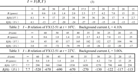
∞ 60 50 45 40 37.5 35 30 25 20 15

B (gauss) 0 0.6 1.0 1.4 2.0 2.3 2.7 4.2 7.0 13 25

I(fA)(B↑) 4.1 9 17 25 34 39 36 26 17 8 2.7

I(fA) (B↓) 4.1 -13 -17 -20 -24 -27 -19 -15 -14 -13 -12

Table 2 I ~ B relation of FX12-51 at t = 10oC. Background current Io = 4.1fA

D (cm) ∞ 60 50 45 40 35 30 25 20 15

B (gauss) 0 0.6 1.0 1.4 2.0 2.7 4.2 7.0 13 25

I(fA) (B↑) 3.0 45 85 117 165 182 152 127 104 94

I(fA) (B↓) 3.0 -53 -72 -78 -59 -43 -26 -22 -20 -17

Table 3 I ~ B relation of FX12-51 at t = 22oC. Background current Io = 3.0fA.

d (cm) ∞ 60 50 45 40 35 30 25 20 15

B (gauss) 0 0.6 1.0 1.4 2.0 2.7 4.2 7.0 13 25

I(fA) (B↑) 7.7 290 560 1360 1530 1650 1270 790 440 250

I(fA) (B↓) 7.7 -520 -670 -690 -670 -270 -130 -122 -117 -115

Table 4 I ~ B relation of FX12-51at t = 33oC. Background current Io = 7.7fA.

temperatures, 10oC, 22oC and 33oC. From t = 10oC to t = 33oC (i.e., from

283K to 306K), the temperature rose only 23oC, nevertheless, the output current increased from 40fA to 1600fA, 40 times! This can be finely

(a)

(b)

explained by Richardson’s equation: thermal electron emission rises very rapidly as the temperature rises,

kT W

e

AT

J



In addition to the output current, electrometer Keithley 6514 together

with the circuit could also be used to measure the output voltage of the

electron tube, as shown in Fig. 11. The highest voltage sensitivity of

Keithley 6514 is 1×10-5V = 0.01mV. The voltage here is actually the

open-circuit voltage of the electron tube, or the electric motive force of

the electron tube.

Fig.11 The output voltage (e.m.f.) measuring circuit.

The following were the output voltages we measured with electron tube FX12-51 in a test at room temperature of t = 25oC (298K):

Background voltage B≈ 0, Uo = 5.6 mV.

When a magnetic field was applied to the tube, the maximum output

voltage (corresponding to an optimum distance d) was also stable

provided the magnet kept stationary. Each maximum output voltage was

B↑≈ 3.5 gauss Umax = 20 21 20 21 mV,

B↓≈ 3.5 gauss Umax = -16 -18 -16 -17 mV。

This output voltage depends on the average kinetic energy of the

thermal electrons of the emitters, that is, depends on the room

temperature. According to Boltzmann’s law of equi-partition of energy,

the average kinetic energy of the thermal electrons at 25oC (298K) is

emV eV

J

kT 1.38 10 298 0.0385 38.5

2 3 2

3 _{  } 23_{  }

 

 ₍₅₎

In expression , the factor 38.5mVis of the same magnitude order

with the output voltage we derived in our measurement (Umax ≈ 17 ～

20mV). That reminded us that the output voltages were surely resulted

from the conversion of part of the kinetic energy of the thermal electrons. emV

5 . 38

We noticed in our tests that the value of the output voltage may be affected considerably by the current leakage between the two emitters. Some of our tubes had very fine insulation between A and B, they might produce higher output voltage, even of 50 ~ 100 mV. We think, such higher voltage was due to the contribution of the thermal electrons of

higher kinetic energy. For example, for electrons of u = 2vrms= 2 v2 , its

kinetic energy is 4×38.5emV = 154 emV.

Both the output current and output voltage of our experiment were very weak. Nevertheless, beyond doubt, they were DC current and DC

voltage, both being macroscopic physical quantities. They were

and in series to increase the output voltage, so as to build up a much greater output power.

Another way to increase considerably the output power of a tube at room temperature is to find new thermal electron emission materials of much lower work functions then Ag-O-Cs.

High temperature cathode materials, such as Ba-Sr-Ca oxides and Cs-Tungsten, etc., may also be used to do such experiments. It needs more skill, money and efforts, but tremendously greater output voltage, current and power will be obtained. In all such experiments, only a single heat reservoir at high temperature is needed, that means, no condenser is needed. Carnot’s principle for the limit of heat engine efficiency will no longer be meaningful. The highest or theoretical possible efficiency of such an apparatus (a new energy converter) is of course one hundred percent. [17]

5. Conclusions

In the above experiment, the heat extracted by electron tube FX12-51 from ambient air converted completely into electric energy without producing other effect. The process proved that the second law of thermodynamics was not absolutely valid, just as Maxwell and Planck

had imagined or predicted in 1871 and 1897, respectively.

The authors maintain: in ordinary thermodynamic processes, just as Clausius and Kelvin pointed out, entropy always increases, never decreases. Nevertheless, in some unconventional or extraordinary thermodynamic processes, such as our experiment of thermal electrons in a magnetic field, entropy does decrease.

REFERENCES

[1] Xinyong Fu, An Approach to Realize Maxwell’s Hypothesis,

Energy Conversion and Management, Vol.22 pp1-3 (1982).

[2] Xinyong Fu and Zitao Fu, Realization of Maxwell’s Hypothesis,

arxiv.org/physics/0311104v1-v3.

[3] Richardson and Brown, Phil. Mag., 16，353 (1908).

[4] Richardson，Phil. Mag., 16，890 (1908); 18, 681 (1909).

[5] L.H.Germer, The Distribution of Initial Velocities among Thermionic

Electrons, Initial Velocities of Thermionic Electrons p. 795 (1925).

[6] Xinyong Fu and Zitao Fu, A Graphical Survey of the Various

Trajectories of Thermal Electrons and Their Contribution to the

Output Current in Fu & Fu’s Heat-Electric Conversion (awaiting

publication)

[7] James Clerk Maxwell, Theory of Heat, Longmans, Green, And Co.

(1888)，P.328

[8] Max Planck, Forlesungen Uber Thermodynamik (Erste auflage,1897;

Siebente auflage,(1922), §116 &§136. English Version: Treatise On

Thermodynamics, Dover Publications Inc. (1926), §116 & §136.

[9] W. Ehrenberg, Maxwell’s Demon, Scientific American, pp 103-110

(1967).

[10] Harvey Leff & Andrew Rex, Maxwell’s Demon: Entropy,

Hilger/British Institute of Physics (1990)

[11] Harvey Leff & Andrew Rex, Maxwell’s Demon 2: Entropy, Classical

and Quantum Information, Computing, Institute of Physics Bristol (2003)

[12] Harvey Leff, Energy and Entropy, A Dynamic Duo, Section 9.5.3,

CRC/Taylor & Francis Group in England (2020)

[13] Koller, L. R., Phys. Rev., 36, 1639 (1930).

[14] Campbell, N. R., Phil. Mag., 12, 173 (1931).

[15] A. H. Sommer, PHOTOEMISSIVE MATERIALS, Preparation,

Properties, and Use, John Wiley & Sons, Section 10.7.1, Chapter 10,

(1968).

[16] John E. Davey, Thermionic and Semiconducting Properties of〔Ag〕

- Cs2O3, Ag, Cs, Journal of Applied Physics, Volume 28, Number 9,

p.1031 (1957).

[17] Kamarul Aizat Abdul Khalid, Thye Jien Leong and Khairudin

Mohamed, Review on Thermionic Energy Converters,