Stoneley Waves At The Interface Of Thermoelastic Diffusion Solid And Microstretch Thermoelastic Diffusion Solid

Aryabhatta Journal of Mathematics and Informatics (Impact Factor- 5.856)

Double-Blind Peer Reviewed Refereed Open Access International e-Journal - Included in the International Serial Directories

Aryabhatta Journal of Mathematics and Informatics

http://www.ijmr.net.in

email id- [email protected]

Page 351 Stoneley Waves At The Interface Of Thermoelastic Diffusion Solid And Microstretch Thermoelastic

Diffusion Solid

Parveen Lata1 and Rajneesh Kumar2 1

Department of Basic and Applied Sciences, Punjabi University, Patiala, Punjab, India 2

Department of Mathematics, Kurukshetra University, Kurukshetra, Haryana, India

Abstract

In this paper, dispersion equation for Stoneley waves at the interface of thermoplastic diffusion solid half space and micro stretch thermoplastic diffusion solid half space have been derived. Numerical computations are performed for a peculiar model to study the variations of phase velocity and attenuation coefficient with respect to wave number. Also the components of normal stress, normal displacement and temperature distribution are obtained and shown with the aid of graphs. Some specific cases are also deduced.

Keywords: Thermoelastic diffusion; Micro stretch; Dispersion equation; Stoneley waves; Propagation characteristics.

1. Introduction

Aryabhatta Journal of Mathematics and Informatics (Impact Factor- 5.856)

Double-Blind Peer Reviewed Refereed Open Access International e-Journal - Included in the International Serial Directories

Aryabhatta Journal of Mathematics and Informatics

http://www.ijmr.net.in

email id- [email protected]

Page 352 thermoelastic diffusion media.Abd-Alla, Khan, and Abo-Dahab[3] and Kumar and Kansal [4] investigated various problems surface waves in viscoelastic fibre-reinforced anisotropic media with voids and in transversely isotropic thermoelastic diffusive plate.Eringen [5] explored microcontinuum field theories. Kumar and Chawla[6] studied wave propagation at the imperfect boundary between the layers of transversely isotropic thermoelastic half-space with diffusion and an isotropic layer .In this paper, dispersion equation for Stoneley waves at the interface of thermoelastic diffusion solid half space and microstretch thermoelastic diffusion solid half space have been derived. Numerical computations are performed for a peculiar model to study the variations of phase velocity and attenuation coefficient with respect to wave number. Also the components of normal stress, normal displacement and temperature distribution are obtained and shown with the aid of graphs. Some specific cases are also deduced.

2. Basic Equations

Following [7,8,9], the governing equations for the problem under consideration can be taken

( ) ( ⃗ ) ( ) ( ⃗ ) ⃗

( ̇) ( ̇) ⃗⃗ , (1) ( ) ( ⃗ ) ( ⃗ ) ⃗ ⃗ ⃗⃗ , (2)

(

) (

) ⃗ , (3) (

) ⃗ ( ) ( )

(

) , (4) ( ⃗ ) (

) ( )

(

) . (5)

and constitutive relations are

(

) (

) ( )

(

Aryabhatta Journal of Mathematics and Informatics (Impact Factor- 5.856)

Double-Blind Peer Reviewed Refereed Open Access International e-Journal - Included in the International Serial Directories

Aryabhatta Journal of Mathematics and Informatics

http://www.ijmr.net.in

email id- [email protected]

Page 353

, (7) , (8)

where

0 1, 0 0

, , , , , , ,

K

    

b



material constants ,







  

1, 2, 3



microrotation vector, *



scalar microstretch function.,



₁



3



2



K





_t1,



₂ 



3



2



K





_c1, ( ) ,

( ) ,

 

t2, t1 coefficients of thermal expansion(linear),

 

c1, c2 coefficients of

diffusion expansion (linear),

j

microintertia, j_o microinertia of the microelements, mij components of couple stress tensors respectively, *

i



microstress tensor, 1 0

,

 

diffusion relaxation times with

0





0





1 ,

 

1, 0 thermal relaxation times with ,

*

K

coefficient of the thermal conductivity.

Here for coupled thermoelastic model



0  

 

1 0  

 

1 1 0,

Lord-Shulman model requires 1

1

0 1

0,

,

1.







 

 







1,



1 



0,

Green-Lindsay (G-L) model requires

0,





0

1







where 0

0



 . 3 Thermoelastic with diffusion

Following [8], the governing equations for a homogeneous isotropic thermoelastic diffusion solid not possessing body forces, heat sources and mass diffusion sources are given by

( ̅ ̅) ( ̅⃗ ) ̅ ( ̅⃗ ) ̅ ( ̅ ̅ ̅̇) ̅ ( ̅ ̅ ̅̇) ⃗⃗

,

(9)

̅̅̅̅ ̅ ̅ ̅ ( ̅ ̅ ) ̅⃗ ̅ ( ̅ ) ̅ ̅ ̅ ( ̅ ) ̅, (10)

̅ ( ̅⃗ ) ̅ ̅ ( ̅

Aryabhatta Journal of Mathematics and Informatics (Impact Factor- 5.856)

Double-Blind Peer Reviewed Refereed Open Access International e-Journal - Included in the International Serial Directories

Aryabhatta Journal of Mathematics and Informatics

http://www.ijmr.net.in

email id- [email protected]

Page 354

(11) and constitutive relations are

̅ ̅ ̅ ( ̅ ̅

) ̅ ( ̅ ̅ ̅̇ ̅ ( ̅ ̅ ̅̇), (12)

4. Problem formulation

We take a homogeneous isotropic generalized thermoelastic diffusion half-space M₁ overlying a homogeneous isotropic microstretch generalized thermoelastic diffusion half-space M2connecting at

the interfacex₃0. The origin of the coordinate system ( ,x x x_{1 2}, ₃)is taken at any point on the plane horizontal surface x₃ 0. We choose the x1-axis in the direction of wave propagation in such a way

that all the particles on a line parallel to the x₂ axis are equally displaced. Therefore, all field quantities are independent of the x₂ coordinate. Medium M₂ occupies the region  x₃0 and the region

3

0x   is occupied by the half-space ofM1. The plane x3 0 represents the interface between two

mediaM₁ andM₂.

We define all the quantities with attached bar for medium M₁and without bar for mediumM₂. For the two dimensional problem, we take

For mediumM2

* *

1 3 1 3 2 1 3

1 3 1 3

( ,

, )

( , 0,

),

(0,

, 0),

( ,

, ),

( ,

, ),

( ,

, ),

u x x t

u

u

x x t

x x t C

C x x t















  



(13)

and, for mediumM₁

1 3 1 3 1 3 1 3

( , , ) ( , 0, ), ( , , ), ( , , ),

u x x t  u u    x x t CC x x t

Aryabhatta Journal of Mathematics and Informatics (Impact Factor- 5.856)

Double-Blind Peer Reviewed Refereed Open Access International e-Journal - Included in the International Serial Directories

Aryabhatta Journal of Mathematics and Informatics

http://www.ijmr.net.in

email id- [email protected]

Page 355 Fig.1. Geometry

Define the dimensionless quantities as

'

'

* *

* * 2 2

' 1 ' 3 ' 1 1 ' 1 3 ' 1 2 * 1 * '

1 3 1 3 2

1 1 1 1 1 1 1

* * *

' ' * ' ' ' 2 ' 2 ' *

2 2

1 1 1 1 1 1 1

' 0' ' 1

, , , , , , ,

, , , , , , , ,

, , ,

ij ij

o o o o o

ij ij i

ij ij i

o o o o o

o

t

x c u

x c u c c

x x u u t

c c T T T T T

t m T T C C

t m T T C C t t

T c T c T T T c c



 



 

_

 

_



_













_

 





_











   

      

       



1'



*



0 1

 

' '



1 *





1 1 3 1 3

1

, , , , , , .

o

o

c

u u u u

T

 

    



 

(15)

where * 2

* 1

* ,

C c K





 2

1

2 K

c







 

 ,

The potential functions

  

, , and



are introduced as

For medium M1 u₁ 

 

_,1 _,3,u₃

 

_,3 _,1, (16)

and, for medium M2 u1

 

,1 ,3,u3

 

,3 ,1, (17)

Putting the values ofu₁ and u₃from (16) in the equations (9)-(11), we obtain x1

O

x2

x3

Thermoelastic diffusion medium M1

Aryabhatta Journal of Mathematics and Informatics (Impact Factor- 5.856)

Double-Blind Peer Reviewed Refereed Open Access International e-Journal - Included in the International Serial Directories

Aryabhatta Journal of Mathematics and Informatics

http://www.ijmr.net.in

email id- [email protected]

Page 356

2 1 1

3 ,

tT a cC

 





    (18)



2



2

1





 

 , (19)

2 0 2 0 0

11 13 ,

e t c

T



a

 

T a



C

     (20)

4 1 2 1 2 0

14 15 t 16 c f 0

a 



a



 T a



 C



C (21) Substituting the values ofu₁ and u₃ from (17) in the equations (1)-(5), we obtain

2 * 1 1

2 t 3 c

,

a

T

a

C



 





 







(22)



2



2

1 2

1







a

 

 , (23)



2



2

4 6 2 5 2,

a a



 a

 

 (24)



2 2



* 2 1 1 *

1 a7 a8 a9 tT a10 cC ,



 



  













(25)





2 0 2 * 0 0

11 12 13 ,

e t c

T



a



a





T a



C

      (26)

4 2 * 1 2 1 2 0

14 21 15 t 16 c f 0,

a  



a 



a



 T a



 C



C (27)

where









12





2

1 2 2 0 3 4 5 6 2 *2 *2 2

1 1 0 1 1

1

1

2

,

,

,

c

,

,

,

,

K

,

K

,

,

a a

K

a

a a a

c

T

j

c

c





 











 















_

_











0 12 1 0 1 14

11 12 13 * *

2

1

,

,

T

,

T

,

c a

a

a

a

K

   















_

_





,





2 *

1 2

14 15 16 2 2

1 1 1

,

,

D

,

a

,

,

a

a

a

b

c

c

















_

_









1 0 1 12 2 14 2 22 2 0 2 2 *

7 8 9 10 *2 1 2 2 21 4

0 1 1 2 0 1 0 1

2

2

,

,

,

,

,

c

,

c

,

c

,

,

D

,

a a a a

c

a

j

T

c

j

c









 

_

  



  

 











_

_











1 1 1 0 0 0

1 0

1,

1,

1,

1,

c t t f

t

t

t

t

















































2 2

0 0 1 3 2

1 0 2 2

1 3 1 3

1

,

1

,

,

.

c e

u

u

e

t

t

x

x

x

x



 







 













 







Aryabhatta Journal of Mathematics and Informatics (Impact Factor- 5.856)

Double-Blind Peer Reviewed Refereed Open Access International e-Journal - Included in the International Serial Directories

Aryabhatta Journal of Mathematics and Informatics

http://www.ijmr.net.in

email id- [email protected]

Page 357 5 Solution of the Problem

We assume the solutions of the form

     

     

     

 

1 1 1

1 1 1

1 1 1

1

* *

2 2

, , ,

, , ,

, , ,

.

i x ct i x ct i x ct

i x ct i x ct i x ct

i x ct i x ct i x ct

i x ct

e T Te C Ce

e e e

e e T Te

C Ce

  

  

  



 

 

 

 









  

  

  



  

  

  



. (28)

where



is the wave number,

 



c

is the angular frequency, and c is phase velocity of the wave. Using (28) in equations (18), (20)–(21) and satisfying the radiation condition



, ,T C0 as x3  ,

we obtain the values of



, ,T C for mediumM1,

 

 

 

1

1 3 2 3 3 3

1

1 3 2 3 3 3

1

1 3 2 3 3 3

1 2 3

1 11 2 12 3 13

1 21 2 22 3 23

(

)

,

(

)

,

(

)

i x ct

m x m x m x

i x ct

m x m x m x

i x ct

m x m x m x

A e

A e

A e

e

T

A n e

A n e

A n e

e

C

A n e

A n e

A n e

e



 



   



  



  



















(29)

where 2 2 2 1, 2, 3

m m m are the roots of the equation

6 * 4 * 2 *

1 1 1 0,

D A D B D C  (30)

* * *

1 12 11

,

1 13 11

,

1 14 11

,

A



d

d

B



d

d

C



d

d

























2

11 11 13 18 12 12 11 11 12 15 13 18 19 2 22

2 2 2

13 13 11 12 12 15 16 13 19 20 2 22 2 23

2 2

14 14 11 13 12 16 17 13 20 21 2 23

, ,

, ,

d l b l d l b l b l b l l a l

d l b l b l l b l l a l a l

d l b l b l l b l l a l













         

        

       

1, 2, 3

A A A are arbitrary constants and

3

.

d

D

dx



Aryabhatta Journal of Mathematics and Informatics (Impact Factor- 5.856)

Double-Blind Peer Reviewed Refereed Open Access International e-Journal - Included in the International Serial Directories

Aryabhatta Journal of Mathematics and Informatics

http://www.ijmr.net.in

email id- [email protected]

Page 358

























6 2 4 2 2 6 4 2

11 22 1 22 23 1 23 24 1 11 1 12 1 13 1

6 2 4 2 2 6 4 2

12 22 2 22 23 2 23 24 2 11 2 12 2 13 2

6 2 4 2 2 6 4 2

13 22 3 22 23 3 23 24 3 11 3 12 3 13 3

,

,

n

l m

l

l

m

l

l

m

l m

l m

l m

n

l m

l

l

m

l

l

m

l m

l m

l m

n

l m

l

l

m

l

l

m

l m

l m

l m















 



  

_









_

_





_



 



  

_









_

_





_



 



  

_









_

_





_

























6 2 4 2 2 2 6 4 2

21 15 1 15 16 1 16 17 1 17 11 1 12 1 13 1

6 2 4 2 2 2 6 4 2

22 15 2 15 16 2 16 17 2 17 11 2 12 2 13 2

6 2 4 2 2 2 6

23 15 3 15 16 3 16 17 3 17 11 3

,

,

,

n

l m

l

l

m

l

l

m

l

l m

l m

l m

n

l m

l

l

m

l

l

m

l

l m

l m

l m

n

l m

l

l

m

l

l

m

l

l m

l





















 



 

_











_

_





_



 



 

_











_

_





_





 

_











_



4 2

12

m

3

l m

13 3

,











and













2 2 2 2

11 23 1 12 1 19 22 12 23 14 13 22 19 1 11 12 14 23 13 21 15 15

2 2 2

14 22 11 21 15 12 13 2 15 15 15 1 14 19 17 23

2 2 2

16 1 12 17 14 19 14 16 18 23 21 19 17

, ( ) , ( ) ,

, ( ),

( ) ,

          

      

     

l b l b b g b g l b b g g g b g a g b

l b g a b g g a g b l a b b b

l g b a b a g g b a g l























14 16 21 19



12 18

2 2 2 2 2

18 14 1 19 1 14 17 22 14 14 20 17 22 1 14 14 14 13 22 18 21 20

2 2

21 14 13 22 18 21 20 22 8 22 14 15 23 14 15 21 22 22 8 23 22 24 ,

, ( ) , ( ) ,

( ), , ( ) ,

 

         

         

a g a g g g

l a l a b b a g l b b a g a g b g a g

l a g b g a g l a b a b l a b g b g a g b g















2 2

11 15 20 16 19 12 23 24 13 14 20 16 18 14 16 18 1 15 14 19 15 18

16 15 20 16 19 18 8 20 16 17 19 8 19 15 17 20 8 18 14 17 21 14 19 15 18 2

22 8 19 15 17 23 22 2

, , , , ,

, , , , ,

, (

g b b b b g b b g b b b b g b b g b b b b

g b b b b g a b b b g a b b b g a b b b g b b b b

g a b b b g b b







         

         

    ₄),g₂₄ a b_{8 18}b b_{14 17},





























2 2 1 1

11 12 1 13 3 14 9 1 15 10

2 2 2 2 2 2 2 2 2

16 1 7 17 11 0 18 0 19 13 1

2 2 2

20 12 0 21 14 22 15 1 23 1

1 , 1, 1 , 1 , 1 ,

, ( ), 1 , ( ),

( ), 2 , 1 ,

b c b i c b a ic b a ic b a ic

b c a b a i c c b c i c b a i c c

b a i c c b a b a ic b a



 

 

 

 





  







  

  



 

            

          

        



1



0

6 ic

 

1 ,b24 i c



(1i

 

c).

We write the appropriate values of *

, , ,T C

Aryabhatta Journal of Mathematics and Informatics (Impact Factor- 5.856)

Double-Blind Peer Reviewed Refereed Open Access International e-Journal - Included in the International Serial Directories

Aryabhatta Journal of Mathematics and Informatics

http://www.ijmr.net.in

email id- [email protected]

Page 359

 

 

 

1

1 3 2 3 3 3 4 3

1

1 3 2 3 3 3 4 3

1

1 3 2 3 3 3 4 3

1 3 2 3 3 3

1 2 3 4

*

1 11 2 12 3 13 4 14

1 21 2 22 3 23 4 24

1 31 2 32 3 33 4 34

( ) ,

( ) ,

( ) ,

(

i x ct

m x m x m x m x

i x ct

m x m x m x m x

i x ct

m x m x m x m x

m x m x m x m

A e A e A e A e e

A n e A n e A n e A n e e

T A n e A n e A n e A n e e

C A n e A n e A n e A n e

















   

   

   

    4 3x _)eix1ct_.

(31)

where

2 2 2 2

1, 2, 3, 4,

m m m m are the roots of the equation

8 * 6 * 4 * 2 *

1 1 1 1 0,

D A D B D C D D  (32)

where * * * 1, 1, 1

A B C and *

1

D are given by,

* * * *

1  12 11, 1  13 11, 1  14 11, 1  15 11, A d d B d d C d d D d d

also

























2

11 11 13 18 12 12 11 11 12 15 13 18 19 2 22

2 2 2

13 13 11 12 12 15 16 13 19 20 2 22 2 23

2 2

14 14 11 13 12 16 17 13 20 21 2 23

2 2 2

15 11 14 12 17 13 21 2 24

,

,

,

,

 



  









  













  





















d

l

b l

d

l

b l

b l

b

l

l

a l

d

l

b l

b

l

l

b

l

l

a

l

a l

d

l

b l

b

l

l

b

l

l

a l

d

b l

b

l

b

l

a

l

a













Aryabhatta Journal of Mathematics and Informatics (Impact Factor- 5.856)

Double-Blind Peer Reviewed Refereed Open Access International e-Journal - Included in the International Serial Directories

Aryabhatta Journal of Mathematics and Informatics

http://www.ijmr.net.in

email id- [email protected]

Page 360













2 2

11 23 1 12 1 19 22 12 23 14

2 2

13 22 19 1 11 12 14 23 13 21 15 15

2 2

14 22 11 2 15 12 13 21 15 15 2

15 1 14 19 17 23

2 2

16 1 12 17 14 19 14 16 18 23 21 19 2 17 , ( ) , ( ) , , ( ), ( ) ,

l b l b b g b g

l b b g g g b g a g b

l b g a b g g a g b

l a b b b

l g b a b a g g b a g

l





















                      





14 16 21 19



12 18 2

18 14 1

2 2

19 1 14 17 22 14 14

2 2

20 17 22 1 14 14 14 13 22 18 21 20 2

21 14 13 22 18 21 20

22 8 22 14 15 2

23 14 15 21 22 22 8 23 22 24 2 24 , , ( ) , ( ) , ( ), , ( ) , (

a g a g g g

l a

l a b b a g

l b b a g a g b g a g

l a g b g a g

l a b a b

l a b g b g a g b g

l

















                     

 a g_{14 21}b g_{22 22})g g_{23 24},

2 2

11 15 20 16 19 12 23 24 13 14 20 16 18 14 16 18 1 15 14 19 15 18

16 15 20 16 19 18 8 20 16 17 19 8 19 15 17 20 8 18 14 17 21 14 19 15 18 2

22 8 19 15 17 23 22 2

, , , , ,

, , , , ,

, (

g b b b b g b b g b b b b g b b g b b b b

g b b b b g a b b b g a b b b g a b b b g b b b b

g a b b b g b b







         

         

    4),g24 a b8 18b b14 17,

The

values of



for medium M x₁( ₃0) and

 

, ₂for M₂(x₃0) satisfying the radiation conditions are

1 

4 3

4 ,

i x ct m x

A e e



_  

(33)

1 

5 3 6 3

5 6

(

A e

m x

A e

m x

)

e

i x ct

,



_

_



(34)

 1 

5 3 6 3

2

(

5 45 6 46

)

i x ct

m x m x

A n e

A n e

e





_

_

 . (35) where 2 2 2

4

(1

2

)

1







c

m





and m m52, 62 are the roots of the equation

4 * 2 *

2 2 0,

D A D B  (36)

Aryabhatta Journal of Mathematics and Informatics (Impact Factor- 5.856)

Double-Blind Peer Reviewed Refereed Open Access International e-Journal - Included in the International Serial Directories

Aryabhatta Journal of Mathematics and Informatics

http://www.ijmr.net.in

email id- [email protected]

Page 361









* 2 2 * 2 2

2 4 24 25(1 ) 1 5 4(1 ) , 2 24 25 1 5 4(1 ) ,

A  a b b 



a a a 



B  b b a a



a 



The roots of equation (31) in the descending order corresponds to the velocities of propagation of three waves viz. longitudinal wave (LW1), thermal wave (TW1) and mass diffusion wave (MW1), respectively.Also, the roots of equation (32) in the descending order corresponds to the velocities of propagation of four possible waves, namely longitudinal displacement wave (LDW2), thermal wave (TW2), mass diffusion wave (MDW2), and longitudinal microstretch wave (LMW2), respectively. Similarly, two roots of the equation (36) corresponds to the coupled transverse displacement and transverse microrotational waves (CDW2- I, CDW2- II) respectively.

(i)

Neglecting diffusion effect, equation (32) leads to sixth order differential equation

6 * 4 * 2 *

3 3 3 0 ,

D A D B D C  ₍₃₇₎

* * *

3 32 31, 3 33 31, 3 34 31,

A d d B d d C d d

























2 2

31 1 32 2 8 16 1 18 11 12 17

2 2 2

33 1 11 18 12 17 16 18 11 12 17 20 8 12 14 2 14 17 8 18 8 2

34 11 14 20 16 18 2 8 18 14 17 12 8 20 16 17

,

,

(

)

(

),

(

)

(

) ,

d

d

a a

b

b

b

b b

d

b b

b b

b

b

b

b b

b

a b

b

a b b

a b

a

d

b

b b

b b

a a b

b b

b a b

b b













 







 









 























and

 

























2 2 1 1

11 12 1 13 3 14 9 1 15 10

2 2 2 2 2 2 2 2 2

16 1 7 17 11 0 18 0 19 13 1

2 2 2

20 12 0 21 14 22 15 1 23 1

1

,

1,

1 ,

1 ,

1 ,

,

(

),

1

,

(

),

(

),

2

,

1 ,

b

c

b

ic

b

a

ic

b

a

ic

b

a

ic

b

c

a b

a i c

c

b

c

i c b

a i c

c

b

a i c

c

b

a b

a

ic

b

a



 

 

 

 





  







  

  



 





 



































 



 





 









1



0

6



ic

 



1 ,

b

24



i c



(1



i

 

c

),

The roots of the equation (37) 2

( 1, 2,3)

p

m p correspond to the LDW2, TW2 and LMW2 waves, respectively.

Clearly on neglecting the diffusion effect, the wave corresponding to this parameter namely mass diffusion wave (MDW2) become deceased.Therefore, it is observed from the equation (32) and (37), that there exist a new type of wave namely MDW2 .

Aryabhatta Journal of Mathematics and Informatics (Impact Factor- 5.856)

Double-Blind Peer Reviewed Refereed Open Access International e-Journal - Included in the International Serial Directories

Aryabhatta Journal of Mathematics and Informatics

http://www.ijmr.net.in

email id- [email protected]

Page 362

4 * 2 *

4 4 0,

D A D B  (38)





2 26

2 0,

1 b D



 

 (39)

* *

4 4

where A and B are given by

* *

4 42 41, 4 43 41,

A d d B d d







2



41 1, 42 18 11 12 17 , 43 11 18 12 17 ,

d  d  b b b b d  b b b b



The roots of the equation (38) correspond to the Longitudinal wave (P-wave), and T waves, and (39) relate to the SV- wave, respectively.

Therefore, it is again observed that there exist new type of wave in (32) namely Longitudinal microstretch wave (LMW2) and transverse microrotational waves (CDW2- II) in (36) which become decoupled in this case .

Substituting the values of

  

, , and



from equations (29), (33) and (30), (34) in equations (16) and (17), we obtained displacement components

For medium M1





 





 

1

1 3 2 3 3 3 4 3

1

1 3 2 3 3 3 4 3

1 1 2 3 4 4

3 1 1 2 2 3 3 4

,

,











   



   







_







_





 

_







_

i x ct

m x m x m x m x

i x ct

m x m x m x m x

u

i

A e

A e

A e

m A e

e

u

m A e

m A e

m A e

i A e

e

(40)

For medium M2



 



 



 



 

1

1 3 2 3 3 3 4 3 5 3 6 3

1

1 3 2 3 3 3 4 3 5 3 6 3

1 1 2 3 4 5 5 6 6

3 1 1 2 2 3 3 4 4 5 6

,

.

i x ct

m x m x m x m x m x m x

i x ct

m x m x m x m x m x m x

u

i

A e

A e

A e

A e

m A e

m A e

e

u

m A e

m A e

m A e

m A e

i

A e

A e

e



















_











_







_











_

(41) 6.Boundary Conditions

Aryabhatta Journal of Mathematics and Informatics (Impact Factor- 5.856)

Double-Blind Peer Reviewed Refereed Open Access International e-Journal - Included in the International Serial Directories

Aryabhatta Journal of Mathematics and Informatics

http://www.ijmr.net.in

email id- [email protected]

Page 363 vanishing of tangential couple stress component, microstretch component, microrotation component. Mathematically, these can be written (at the boundary surfacex₃ 0) as

(i).t33 t33, (42)

(ii).t31 t31, (43) (iii). m32 0, (44) (iv). *

3 0,



 (45)

(v). u3 u3, (46) (vi).u1 u1, (47)

(vii).

T



T

(48)

(viii).

C



C

(49)

(ix). * *

3 3

,

T

T

K

K

x

x







_





_



_





(50)

(x). * *

3 3

,

C

C

D

D

x

x



_







(51)

7 Derivations of the secular equations

Making use of equations (29),(30),(33),(34),(40) and (41) in the equations (42)-(51) with the aid of (6)-(8),(12) and (15), we obtain

4 6

, 4

1 1

0, 

 

 



qp p



q p p

p p

k A k A for

1

 

q

10

(52)

Aryabhatta Journal of Mathematics and Informatics (Impact Factor- 5.856)

Double-Blind Peer Reviewed Refereed Open Access International e-Journal - Included in the International Serial Directories

Aryabhatta Journal of Mathematics and Informatics

http://www.ijmr.net.in

email id- [email protected]

Page 364

























2 2 1

1 2 1 2 1 3

1 1

2 2 1

4 1 2 1, 4 2, 4 1 3, 4

4 1

1 1 1 , 1 3,

1 , 4,

,

1 1 , 5 8,

1 , 9 10.

p p p p

p p

p p p p

p

m b a n n ic n ic p

im b p

k

m b a n n ic n ic p

im b p



 

 





 

 



                   _{ }                   

















2 3 2 2 2 3 2

4 2 3

2 2

2 4 3 1 4, 4

, 1

3,

,

4,

,

, 5

8,

, 9

10.

p

p p

p

p p

i m

b

b

p

b m

b

p

k

i m

b

b

p

b m

b

a n

p









  



_

_

_{ }





_

_

_



 



 









 



3

5 1, 4

4 4, 6 4

0, 1

3,

0,

4,

,

, 5

8,

, 9

10.

p p p p

p

p

k

i b n

p

b n

m

p



_  

 





_



  

_

 



 



4

6 4 1, 4

5 4, 4

0, 1

3,

0,

4,

,

, 5

8,

,

9,

p p p p

p

p

k

b m

n

p

i b n



p

  

 





_



 

_{ }



 





5 4

0, 1

3,

0,

4,

,

, 5

8,

,

9

p p

p

p

k

m

p

i



p



 





_



 

_{ }





_



6 4

, 1

3,

,

4,

,

, 5

8,

,

9.

p p p

i

p

m

p

k

i

p

m

p







 





_



 

_

 







2 7 2, 4

,

1

3

0,

4,

,

,

5

8

Aryabhatta Journal of Mathematics and Informatics (Impact Factor- 5.856)

Double-Blind Peer Reviewed Refereed Open Access International e-Journal - Included in the International Serial Directories

Aryabhatta Journal of Mathematics and Informatics

http://www.ijmr.net.in

email id- [email protected]

Page 365 3

8

3, 4

,

1

3,

0,

4,

,

,

5

8,

0,

9

10,

p

p

p

n

p

p

k

n

p

p



 





_



 

_

_{ }





_{ }



*

2

9 *

4 2, 4

,

1

3,

0,

4,

,

,

5

8,

0,

9

10.

p p

p

p p

K m n

p

p

k

K m

n

p

p

 



 



_



 

_{ }





_{ }



*

3

10 *

4 3, 4

,

1

3,

0,

4,

,

,

5

8,

0,

9

10,

p p

p

p p

D m n

p

p

k

D m

n

p

p

 



 



_



 

_{ }





_{ }



2 2

2

0 0

1 2 2 2 3 2 4 2 5 2 6 2

1 1 1 1 1 1

,

,

,

,



,

 

.







 



















K







b



b

b

b

b

b

b

c

c

c

c

c

c

The system of equations (52) has a non-trivial solution if the determinant of amplitudesA_p,A_pvanishes leading to the secular equation

10 10 0 , , (1, 2,3,...,10)

ij

k for i j

   (53)

Equation (53) is the dispersion equation for the Stoneley wave propagation at an interface between thermoelastic diffusion and microstretch thermoelastic diffusion solid half spaces.

8 Particular Cases

(i) Ignoring the diffusion effect, the dispersion equation for the propagation of Stoneley waves at an interface between thermoelastic and microstretch thermoelastic solid half spaces is obtained as

(ii)

8 8 0 , (1, 2,3,...,8)

ij

k for i j

  

Aryabhatta Journal of Mathematics and Informatics (Impact Factor- 5.856)

Double-Blind Peer Reviewed Refereed Open Access International e-Journal - Included in the International Serial Directories

Aryabhatta Journal of Mathematics and Informatics

http://www.ijmr.net.in

email id- [email protected]

Page 366













2 2

1 2 1

1

1 _{2 2}

3 1 2 1, 3 2, 3 1

3 1

, 1, 2

1 , 3

, 1 , 4, 5, 6

1 , 7,8

p p

p p

p p p

p

m b a n p

i m b p

k

m b a n n i c p

i m b p







 



                     _{ } 

















2 3 2 2 2 3 2

3 2 3

2 2

2 3 3 1 4, 3

,

1, 2

,

3

,

,

4,5, 6

,

7,8

p p p p p p

i m

b

b

p

b m

b

p

k

i m

b

b

p

b m

b

a n

p









  













_

_

_



 

















3 3

0,1

2

0,

3

,

, 4

6

, 7

8

p p

p

p

k

m

p

i



p



 





_



 

_{ }





_{ }



4 3

, 1

2)

,

3

,

, 4

6

, 7

8

p p p

i

p

m

p

k

i

p

m

p







 





_



  

_

 



 



5

5 1, 3

4 4, 3 3

0, 1

2)

0,

3

,

, 4

6

, 7

8

p p p p

p

p

k

i b n

p

b n

m

p



  

 





_



  

_

 



 



6

6 5 1, 3

5 4, 3

0, 1

2

0,

3

,

, 4

6

, 7

8

p p p p

p

p

k

b m

n

p

i b n



p

  

 





_



 

_{ }



 

 



7 4, 3

0,

1

2

0,

3

,

0,

4

6

,

7

8

p p

p

p

k

p

n

_

p

 





_



 

_{ }





 



8 *

3 2, 3

0,

1

2

0,

3

,

,

4

6

0,

7

8

p

p p

p

p

k

K m

n

p

p

 

 





_



 

_{ }





_{ }



(ii) Neglecting thermal and diffusion effects, the dispersion equation (54) reduced to theStoneley wave propagation at an interface of elastic/microstretch elastic solid half spaces.

(iii) Take



0 _0,





₀

_and 0 1







in equation (54), yield the corresponding expressions with two relaxation times.

(iv) Using



1  



1 0,



0 



1,and





1

in equations (54),gives the corresponding results with one relaxation time.

Aryabhatta Journal of Mathematics and Informatics (Impact Factor- 5.856)

Double-Blind Peer Reviewed Refereed Open Access International e-Journal - Included in the International Serial Directories

Aryabhatta Journal of Mathematics and Informatics

http://www.ijmr.net.in

email id- [email protected]

Page 367 9 Numerical results and discussion

Persuing [9], the values of micropolar parameters for medium M1(magnesium)are taken as

9 -2 9 -2 2 3

94 10 Nm , 40 10 Nm , 17.4 10 Kgm ,



_{ }



_{ }



_{ } 

3 2 2 -1 * 3 1 1 6 -1

t1 0

5 3 -1 5 3 -1

1 c1 c2

5 -1 5 2 1 8 3 * 5 1 1 1

* 0

t2

29 10 m s K ,

1.04 10

,

23.3 10 K ,

0.02,

0.01,

26.5 10 m Kg ,

28.3 10 m Kg ,

32 10 Kg m s ,

0.04,

0.85 10

, K

17 10

,

1.5,

0.03,

24.8 10

a

C

JKg K

b

D

Kgm s

Jm s K



















   

 

     



































 









6 -1

K .



and for medium M2, data are given by

10 -2 10 -2 10 2

3 3 19 2 9

0.759 10 Nm ,

0.189 10 Nm ,

1.49 10

,

2.190 10

,

0.196 10

,

0.268 10



  

























K

Nm

Kgm

j

m

N









Thermal and diffusion parameters are given by

* 2 1 1 * 5 1 1 1 6 -1 6 -1

t1 t2

2 2 * 5 1 1 1 5 3 -1 5 3 -1

0 1 0 c1 c2

4 2 2 -1 5

11.8 10

, K

15 10

,

22.2 10 K ,

23.8 10 K ,

19.8 10K,

0.9 10 ,

1 10 , K

15 10

,

23.4 10 m Kg ,

26.1 10 m Kg ,

2.32 10 m s K ,

30.61 10 Kg

C

JKg K

Jm s K

T

Jm s K

a

b













      

      







 













 

 

 

















-1 5 2 1 * 1 0 2

10 3

m s ,

0.03,

14.8 10 ,

2 10 .

63 10

,

D

Kgm s







  

 







 

 

and the microstretch parameters are taken as

21 2 10 2 10 9 2 10

1

16.5 10

,

0.37 10

,

6.1 10

,,

3.7 10

,

2.5 10

.

o o o o

j







m







Nm











N







Nm



b







N

Above data has been used for numerical computation of the resulting quantities.

Fig.2 shows that phase velocity initially decreases sharply, attains minima and then shows a stationary behavior. Also the values of phase velocity decreases under the effect of diffusion.

Fig.3 shows that in absence of diffusion effect, attenuation coefficient increases smoothly with increase in wave number for LS and GL theories. While under the effect of diffusion, minimum variation is observed in the magnitude values of attenuation coefficient which appears to be stationary.

Fig.4 shows that initially small variation is observed in the magnitude values of normal displacement u3

Aryabhatta Journal of Mathematics and Informatics (Impact Factor- 5.856)

Double-Blind Peer Reviewed Refereed Open Access International e-Journal - Included in the International Serial Directories

Aryabhatta Journal of Mathematics and Informatics

http://www.ijmr.net.in

email id- [email protected]

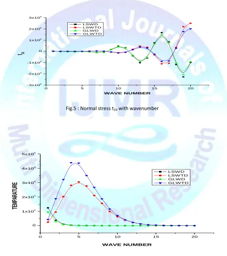
Page 368 Fig.5 depicts that normal stress t33 fluctuates with wave number. This fluctuation increases with

increase in the wave number. Values are maximum when diffusion is absent. Initially under the effect of diffusion the values of displacement starts with an initial decrease.

Fig.6 depicts that magnitudes of temperature for LS and GL theories under the effect of diffusion initially decreases and then shows a stationary behavior. But if there is no diffusion, a sharp increase and smooth decrease in values is observed till it becomes stationary.

10 Conclusion

In the present Chapter, frequency equation for the Stoneley waves at bounded interface is derived in the compact form by using appropriate boundary conditions. It is found that Stoneley waves in the considered model are dispersive. Computer algorithm has been developed for a particular model for numerical. Numerically simulated results are depicted with the aid of graphs to study the variation of phase velocity and attenuation coefficients with respect to wavenumbers. It is seen that for small values of non-dimensional wavenumber, the effect of different relaxation times have a significant effect on dispersion curve and less effect is seen for higher value.

Fig.2 : Phase velocity with wavenumber

0

5

10

20

-1.5x10

1.5x10

-1

-1

1

7.5x10

-1

8.5x10

-1

V

E

L

O

C

I

WAVE NUMBER

LSWD

LSWTD GLWD

Aryabhatta Journal of Mathematics and Informatics (Impact Factor- 5.856)

Double-Blind Peer Reviewed Refereed Open Access International e-Journal - Included in the International Serial Directories

Aryabhatta Journal of Mathematics and Informatics

http://www.ijmr.net.in

email id- [email protected]

Page 369 Fig.3 : Attenuation Coefficient with wavenumber

0 5 10 15 20

-3x105 -2x105 -1x105 0 1x105 2x105 3x105

u

3

WAVE NUMBER

LSWD LSWTD GLWD GLWTD

0

5

1

1

2

0.2x10

2.2x1

1

4.2x1

1

6.2x1

1

8.2x1

1

9.2x1

1

10.2x1

1

ATTENUATION COEFFCIENT

WAVE NUMBER

LSWD

Aryabhatta Journal of Mathematics and Informatics (Impact Factor- 5.856)

Double-Blind Peer Reviewed Refereed Open Access International e-Journal - Included in the International Serial Directories

Aryabhatta Journal of Mathematics and Informatics

http://www.ijmr.net.in

email id- [email protected]

Page 370 Fig. 4: u3 with wavenumber

Fig.5 : Normal stress t33 with wavenumber

0 5 10 15 20

-3x106

-2x106

-1x106

0 1x106

2x106

3x106

t

33

WAVE NUMBER

LSWD LSWTD GLWD GLWTD

0 5 10 15 20

0 1x104

2x104

3x104

4x104

5x104

TE

MP

AR

AT

UR

E

WAVE NUMBER