Tuning Stencil Codes in OpenCL for FPGAs.

(1)

ABSTRACT

JIA, QI. Tuning Stencil Codes in OpenCL for FPGAs. (Under the direction of Dr. Huiyang Zhou).

OpenCL is designed as a parallel programming framework to support heterogeneous computing platforms. The implicit or explicit parallelism in OpenCL kernel code enables efficient FPGA implementation from a high-level programming abstraction. However, FPGA architecture is completely different from GPU architecture, for which OpenCL is widely used. Tuning OpenCL codes to achieve high performance on FPGAs is an open problem and the existing OpenCL tools and optimizations proposed for CPUs/GPUs may not be directly applicable to FPGAs. A detailed study on OpenCL code optimizations for stencil computations on FPGAs and characterization on FPGA memory systems is presented in this thesis.

(2)

(3)

Tuning Stencil Codes in OpenCL for FPGAs

by Qi Jia

A thesis submitted to the Graduate Faculty of North Carolina State University

in partial fulfillment of the requirements for the degree of

Master of Science

Electrical and Computer Engineering

Raleigh, North Carolina 2016

APPROVED BY:

_______________________________ _______________________________ Dr. Huiyang Zhou Dr. Gregory Byrd

Committee of Chair

(4)

DEDICATION

(5)

BIOGRAPHY

(6)

ACKNOWLEDGMENTS

I would like to express my thanks to Dr. Huiyang Zhou for his persistent, helpful and kind guidance, discussions and suggestions since I joined the group. I would also like to thank Dr. Gregory Byrd and Dr. Xipeng Shen for serving on my thesis committee and all the helpful feedbacks of my work.

I am also thankful to all my colleagues: Hongwen Dai, Xiangyang Guo, Chao Li and Zhen Lin for their discussions about my work.

(7)

TABLE OF CONTENTS

LIST OF TABLES ... vii

LIST OF FIGURES ... ix

1. Introduction and Motivation ... 1

1.1. Introduction on OpenCL for FPGAs ... 1

1.2. Importance of Stencil Computations ... 3

1.3. Stencil in OpenCL for FPGAs ... 3

2. OpenCL Architectures for FPGAs ... 5

3. Tuning OpenCL Stencil Codes for FPGAs ... 9

3.1. Optimizing Single-Task Kernels ... 9

3.2. Optimizing NDRange Kernels ... 13

3.3. Comparison with Optimizations for GPUs ... 18

4. Characterizing FPGA Memory Systems ... 20

4.1. Global Memory and LSU Embedded Caches ... 21

4.2. Constant Caches ... 21

4.2.1. Constant Cache Access Vectorization ... 22

4.3. Local Memory ... 24

4.3.1. Local Memory Access Vectorization... 25

4.4. Constant Cache vs LSU Embedded Cache ... 26

5. Experiments ... 27

5.1. Experiment Setup ... 27

(8)

5.3. 2D Convolution ... 32

5.4. 2D Jacobi Iteration ... 34

5.4.1. 2D Jacobi Iteration in Shape 0 ... 35

5.5. 3D Jacobi Iteration ... 41

5.6. Comparison with Altera Design Examples ... 47

6. Related Work ... 48

(9)

LIST OF TABLES

(10)

(11)

LIST OF FIGURES

Figure 1 FPGA Internal Structure……….……..1

Figure 2 2DConv Kernel Performance Improvements over the Baseline from Different Optimizations……….…….5

Figure 3 The Altera OpenCL for FPGA Architecture………....6

Figure 4 Compute Unit Structure of Vector Addition……… …….……..7

Figure 5 The Tuning/Optimization Process for Single-task Kernels………..10

Figure 6 A Code Snippet of a 1DConv Single-Task Kernel Using SRP………….………..10

Figure 7 A Code Snippet of a 1DConv Single-Task Kernel Using SRP and TAC…….…..12

Figure 8 The Tuning/Optimization Process for NDRange Kernels………...……14

Figure 9 A Code Snippet of a 1DConv NDRange Kernel using LM……….…………...…16

Figure 10 2DConv Kernel Execution Time with Variable Local Memory Sizes (the lower, the better)………...…….………….16

Figure 11 A Code Snippet of a 1DConv NDRange Kernel using LM and VEC……...…..17

Figure 12 Optimized 1DConv NDRange Kernel………..….………19

Figure 13 Array Initialization in Pointer-chasing Benchmark………...………20

Figure 14 Constant Cache Latency and Frequency with Different Number of Ports....……22

Figure 15 System Speedup over Baseline for 1Dconv NDRange Kernel with Different Vector Data Types……….23

(12)

Figure 17 Local Memory Latency and Frequency with Different Memory Size...…….…..25

Figure 18 Local Memory Latency and Frequency with Different Port Width……….…….26

Figure 19 2D Jacobi Iteration in Shape 0……….…….28

Figure 22 3D Jacobi Iteration Algorithms………...……….…….29

Figure 23 Speedups and Energy consumption of 1DConv after Applying Optimizations in the Single-Task Mode……….30

Figure 24 Speedups and Energy Consumption of 1DConv after Applying Optimizations in the NDRange Mode……….………….31

Figure 25 Speedups and Energy Consumption of 2DConv after Applying Optimizations in the Single-Task Mode………...…………32

Figure 26 Speedups and Energy Consumption of 2DConv after Applying Optimizations in the NDRange Mode……….…….33

Figure 27 Speedups and Energy Consumption of 2D Jacobi in Shape 0 after Applying Optimizations in the Single-Task Mode………...……35

Figure 28 Speedups and Energy Consumption of 2D Jacobi in Shape 0 after Applying Optimizations in the NDRange Mode………..……36

Figure 29 Speedups and Energy Consumption of 2D Jacobi in Shape 1 after Applying Optimizations in the Single-Task Mode………...………37

(13)

Figure 31 Speedups and Energy Consumption of 2D Jacobi in Shape 2 after Applying

Optimizations in the Single-Task Mode……….……….……39

Figure 32 Speedups and Energy Consumption of 2D Jacobi in Shape 2 after Applying Optimizations in the NDRange Mode……….………40

Figure 33 3D Blocking Optimization……….….……42

Figure 34 2.5D Blocking Optimization……….…..………43

Figure 35 2.5D Blocking Optimization Codes………....……44

Figure 36 Speedups and Energy Consumption of 3D Jacobi after Applying Optimizations in the Single-Task Mode……….……45

Figure 37 Speedups and Energy Consumption of 3D Jacobi after Applying Optimizations in the NDRange Mode………46

(14)

1. Introduction and Motivation

1.1. Introduction on OpenCL for FPGAs

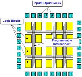
Figure 1 FPGA Internal Structure

(15)

describe a circuit using Verilog or VHDL and the programmability of FPGAs using Verilog or VHDL is a major hurdle for them to be widely adopted.

From the last decade in last century to the present day, there has been an increasing interest and effort in research on high-level synthesis (HLS), because describing a circuit in high-level language is much more convenient compared to an equivalent Verilog or VHDL description, which can ease the burden of FPGA engineer to a large degree.

Traditional HLS tools implement a circuit from high-level language like C. They implement a circuit in a single-instruction single-data (SISD) fashion, comprising a datapath that performs computation and a control circuit that schedules the flow of computation. The performance can be optimized by scheduling independent instructions simultaneously. However, this approach does not make full use of FPGA resources. First, it is possible that many such circuits can be placed on FPGA and they can simultaneously process data, which increases the overall throughput of a design. Second, parallelism cannot be expressed explicitly in programming languages such as C, and thus it is not always possible to generate a circuit that has a comparable performance to a design written manually in Verilog/VHDL.

(16)

kernel may be replicated to further improve performance of the application based on the available resources on FPGA device.

Although using OpenCL significantly improves the programmability of FPGAs, how to write high performance OpenCL code for FPGAs remains a critical challenge. The reason is that the architecture of FPGAs generated from OpenCL code is fundamentally different from that of CPUs/GPUs, on which the existing OpenCL tools and optimizations mainly focus. Therefore, it is crucial to understand the FPGA architectures and the characteristics of FPGA on-chip resources in order to optimize OpenCL code for FPGAs.

1.2. Importance of Stencil Computations

Stencil (nearest-neighbour) computations are a class of iterative kernels which update array elements according to some fixed pattern, called stencil.

Stencil computations are an important class of algorithms at the heart of many calculations involving structured (i.e., rectangular) grids, including implicit and explicit partial differential equation (PDE) solvers. Besides their importance in scientific computing, stencils are interesting as an architectural evaluation benchmark due to their abundant parallelism and low computational intensity, offering a mix of opportunities for parallelism and challenges for memory systems.

1.3. Stencil in OpenCL for FPGAs

(17)

smartphones. Most of the existing works [4][8][11][15] are primarily designed for CPUs/GPUs. Unfortunately, many of these schemes may not be directly applied to FPGAs. Although there are also prior works [6][10][16] focusing on customizing stencil computations on FPGAs, they mainly utilize hardware description languages while our focus is the high-level OpenCL framework. To the best of our knowledge, this is the first work on tuning stencil codes in OpenCL for FPGAs.

In this thesis, the 1D/2D/3D stencil codes are tuned using different optimizations in the two modes supported in the Altera OpenCL for FPGA framework, NDRange Kernels and Single-Task Kernels (aka Single-Work-Item Kernels). It is also revealed how different types of memory (i.e. constant memory and local memory) will be affected by OpenCL code patterns on FPGAs.

As shown in a previous work [18], tuning OpenCL program code has a remarkable performance impact on the synthesized FPGAs. This study confirms the case for OpenCL stencil codes. Using the 2D convolution (2DConv) as an example, the OpenCL code is optimized with different optimizations. The normalized performance speedups from these optimizations (details of the optimizations are shown in later sections) are shown in Figure 2. From the figure it can be seen that the optimized version can be over two orders of magnitude faster than the baseline (i.e., un-optimized) code. This highlights the importance of OpenCL code optimizations for FPGAs.

(18)

Second, we reveal details about how different types of memory on FPGAs are generated and their corresponding performance characteristics.

Figure 2 2DConv Kernel Performance Improvements over the Baseline from Different Optimizations

The remainder of the thesis is organized as follows. In Section 2 we introduce the OpenCL architectures on FPGAs. We propose the performance tuning processes for stencil codes in Section 3. We characterize different types of memory resources on FPGAs in Section 4. Section 5 analyzes our experiments results. We compare our work with previous related work in Section 6. Finally, Section 7 concludes the thesis.

2. OpenCL Architectures for FPGAs

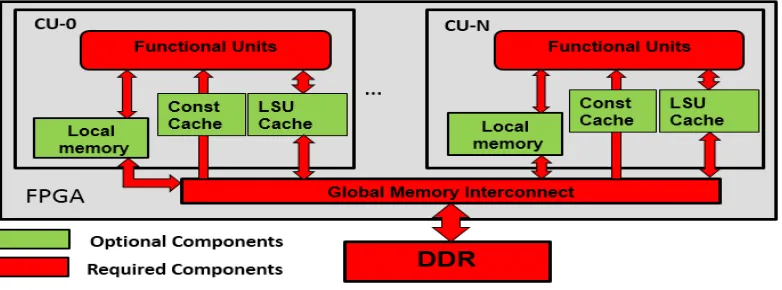
Recently developed OpenCL frameworks for FPGA, such as the Altera SDK for OpenCL [1], enable a user to replace/augment the traditional hardware FPGA design flow with a much faster and higher-level software development flow. Instead of treating FPGAs as pure hardware resources such as look-up tables (LUTs), registers, DSP blocks and memory blocks, the OpenCL for FPGA architecture is a massive parallel computing engine, as shown

0 40 80 120 160

baseline opt1 opt2 opt3 opt4 opt5

S

pe

(19)

in Figure 3. The generic OpenCL for FPGA architecture consists of one or more compute units (CUs), different types of memory and the interconnects among them.

Figure 3 The Altera OpenCL for FPGA Architecture

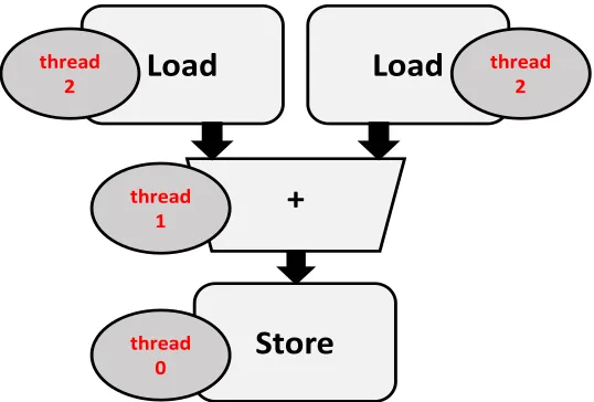
Each instruction in an OpenCL kernel is translated into a functional unit, e.g., an adder or a load-store unit (LSU), and a multi-instruction sequence is synthesized into a pipeline of functional units. The key to achieve high throughput is to convert thread-level parallelism in NDRange kernels or loop-level parallelism in Single-Task kernels into pipeline parallelism. The pipeline synthesized from a kernel is referred to as a Compute Unit (CU). Each CU provides pipelined execution for massive threads/loop iterations of an OpenCL kernel. Figure 4 shows the CU structure of a vector addition kernel (C=A+B) as an example. The pipeline depth indicates how many threads/work-items can run concurrently in the different pipeline stages. In Figure 4, up to three threads/work-items can run concurrently and the peak throughput is one thread/work-item finishing each cycle.

(20)

global memory have long latencies, and the bandwidth is shared by all the CUs on the FPGA. The data in global memory can be buffered in on-chip caches embedded within LSUs. Second, local memory is a low-latency and high-bandwidth software-managed scratchpad memory. Third, constant memory also resides in off-chip DRAM on the FPGA board while its data can be buffered in on-chip constant caches. Fourth, private memory, storing private variables or small arrays for each work-item, is implemented using on-chip registers and has the fastest speed. Among the four types of memory, private memory and local memory are rather plentiful on FPGAs, compared to GPUs. Constant caches and LSU embedded caches are optional and initiated when the compiler determines that their existence improves the performance.

Figure 4 Compute Unit Structure of Vector Addition

There are typical OpenCL features [2][3] presented in the Altera OpenCL for FPGA programming/optimization guide so that programmers are able to perform performance optimizations on the OpenCL kernels.

Load

+

Store

thread

0 thread

1

thread 2 thread

(21)

Local Memory (LM): To alleviate the stalls on global memory accesses, local memory can be utilized to reduce the total number of global memory transactions and provide low-latency, high-bandwidth accesses.

Loop Unrolling (LU): The loop iterations are possibly the critical path of a kernel pipeline if there is a large amount of loop iterations existing in the kernel pipeline. LU decreases the total number of iterations at the expense of increased hardware resource consumption. Also, in some occasions LU also helps the compiler to detect memory coalescing opportunities. The load/store operations can be coalesced so that the total number of global memory transactions is reduced.

Kernel Vectorization (SIMD): To achieve higher throughput, the OpenCL kernel can be vectorized at the expense of more hardware resource consumption. Kernel vectorization allows multiple work items to execute in a single instruction multiple data (SIMD) fashion. Multiple scalar arithmetic operations will be translated to a single vector arithmetic operation once SIMD is applied. With SIMD, the number of total work items can be reduced. Similar to LU, kernel vectorization also helps with the memory coalescing, which will reduce the total number of global memory transactions.

(22)

from different CUs cannot be coalesced, they will compete for limited global memory bandwidth and probably causes performance degradation due to global memory accesses congestion.

In this work, we propose the tuning process to streamline those optimizations mentioned above and highlight the importance of additional optimizations such as thread/task coarsening.

3. Tuning OpenCL Stencil Codes for FPGAs

The OpenCL kernels for Stencil codes on FPGAs can be implemented in either the Single-Task mode or the NDRange mode [2]. We propose somewhat different optimization processes and present them separately.

3.1. Optimizing Single-Task Kernels

In the Single-Task mode, a kernel is implemented as a sequential program and the host will execute the kernel as a single work item. The compiler, e.g., the Altera Offline Compiler (AOC), extracts the loop-level parallelism to enable pipelined execution. Our proposed optimization process for stencil kernels in the Single-Task mode is shown in Figure 5. It consists of both memory architecture tuning and computation pipeline tuning. As the stencil kernels’ performance on FPGAs is eventually bound by memory, memory architecture is tuned before computation pipelines.

(23)

Figure 5 The Tuning/Optimization Process for Single-task Kernels

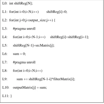
Figure 6 A Code Snippet of a 1DConv Single-Task Kernel Using SRP L0: int shiftReg[N];

L1: for(int i=0;i<N;i++) shiftReg[i]=0; L2: for(int j=0;j<output_size;j++) {

L3: #pragma unroll

L4: for(int i=0;i<N-1;i++) shiftReg[i]=shiftReg[i+1]; L5: shiftReg[N-1]=srcMatrix[j];

L6: sum = 0; L7: #pragma unroll L8: for(int i=0;i<N;i++)

L9: sum += shiftReg[N-1-i]*filterMatrix[i]; L10: outputMatrix[j] = sum;

(24)

Putting data in constant memory can leverage constant caches, whose performance is dependent on the cache hit rates. In stencil codes, there are some small-size and frequently-accessed data, such as the filter matrices in 1D/2D convolution. Putting these small matrices into constant memory is a natural optimization on GPUs. But for FPGAs, the decision between putting them into either global memory or constant memory is more delicate and we need to take both the matrix sizes and access patterns into consideration. We will discuss the impact from different types of memory in Section 4.

Applying SRP on Single-Task kernels can improve the memory access efficiency significantly for the following two reasons. First, shift registers help to make use of the data temporal locality in stencil codes by buffering the data in registers, which can reduce the global memory accesses significantly. Take 1D convolution (1DConv) as an example. Figure 6 shows a snippet of the 1DConv Single-Task kernel after applying SRP. From line 3 to line 5, we shift one element and insert a new element from the input, srcMatrix. In line 8, the shift registers are used to perform the computation. All the elements in the srcMatrix are loaded from global memory only once and fully reused before they are shifted out. Assume the outputMatrix and srcMatrix have N elements while the size of filterMatrix is M. Then after applying SRP, the number of global memory accesses is decreased from N*M to N. Second, as stated in [2], the shift register accesses are more efficient than on-chip block RAMs accesses. It is worth indicating that in line 3 and line 7, ‘#pragma unroll’ is necessary for AOC to infer the shift registers.

(25)

inner loops deepens the synthesized pipeline and enables more outer-loop iterations to be in the pipeline simultaneously, thereby improving the throughput.

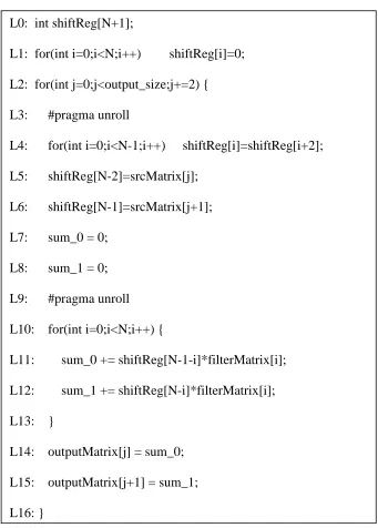
Figure 7 A Code Snippet of a 1DConv Single-Task Kernel Using SRP and TAC L0: int shiftReg[N+1];

L1: for(int i=0;i<N;i++) shiftReg[i]=0; L2: for(int j=0;j<output_size;j+=2) { L3: #pragma unroll

L4: for(int i=0;i<N-1;i++) shiftReg[i]=shiftReg[i+2]; L5: shiftReg[N-2]=srcMatrix[j];

L6: shiftReg[N-1]=srcMatrix[j+1]; L7: sum_0 = 0;

L8: sum_1 = 0; L9: #pragma unroll L10: for(int i=0;i<N;i++) {

L11: sum_0 += shiftReg[N-1-i]*filterMatrix[i]; L12: sum_1 += shiftReg[N-i]*filterMatrix[i]; L13: }

(26)

Besides deepening the pipeline, the throughput can be improved with widening the pipeline. For example, rather than producing one output, outputMatrix[j], per iteration in the outer loop (line 2 in Figure 6), we can generate multiple outputs per iteration. We refer this optimization as task coarsening. Task coarsening is apparently similar to unrolling and jamming the outer loop in Figure 6. But there is a subtle but important difference. Considering task coarsening with a factor of two, i.e., we want each outer loop iteration computes two outputs, i.e., outputMatrix[j] and outputMatrix[j+1]. Although this can be achieved by unrolling and jamming the outer loop enclosed between line 2 and line 11, a more efficient way is to change the size of the shift register at line 0, ‘int shiftReg[N+1]’, and shift the registers by two at a time, i.e., ‘shiftReg[i]=shiftReg[i+2];’ at line 4. The codes after applying TAC are shown in Figure 7. Our experiments confirm that for 1DConv, such manual TAC outperforms unrolling the outer loop with ‘#pragma unroll’ by 25.3% when the coarsening (or unroll) factor is 8.

3.2. Optimizing NDRange Kernels

In the NDRange mode, the algorithms need to be parallelized into separate work-items (or threads). In other words, the thread-level parallelism needs to be expressed explicitly by programmers. Figure 8 shows our optimization process for stencil kernels in the NDRange mode, which is also composed of memory architecture tuning and computation pipeline tuning, similar to the Single-Task mode.

(27)

similar to what we discuss for Single-Task kernels. VEC is applied in the final stage in memory architecture tuning since the memory access type needs to be known before the accesses are vectorized.

Figure 8 The Tuning/Optimization Process for NDRange Kernels

Local memory can be used as software managed caches to reduce the number of global memory accesses. It is appropriate for stencil codes due to their strong data reuses. Figure 9 shows the LM optimization for 1DConv NDRange kernel, which is similar to shared memory optimization on GPUs. On GPUs, a programmer typically aims to make use of all available shared memory resources as long as shared memory is not the limiting factor for thread-level parallelism. But it is a different story on FPGAs. The kernel performance on FPGA does not always favor large local memory sizes. Take 2DConv as an example. We set the filter matrix size as 17x17 and the work group size as NxN. Then the local memory size needs to be (N+16)x(N+16). The larger the local memory size is, the more data reuses will be captured by local memory, which helps to improve the system performance. But if N is larger than 16, some of the work-items will be idle when loading elements in the halo from global memory into local memory. As the total execution time of the kernel on FPGAs is

Constant Memory Apply Naïve

Kernel OptKernel

Local Memory

Apply

Loop Unrolling

Memory Architecture Tuning Computation Pipeline Tuning Vectorization _CoarseningThread

(28)

determined by the total number of work-items instead of active work-items, the inactive work-items still cause overhead, hurting the system performance. Figure 10 shows the 2DConv kernel execution time using various local memory sizes (the kernel only makes use of local memory and does not use other optimizations) with the filter size 17x17. From Figure 10, it can be seen that when the local memory size is 32x32 (i.e., the workgroup size is 16x16), the performance is the best. So, when applying local memory optimization on OpenCL kernels on FPGAs, the local memory size should be determined by the filter size and workgroup size.

Vectorization helps to coalesce memory accesses to utilize the global memory bandwidth efficiently. Originally as stated in [3], memory coalescing refers to combining multiple consecutive global memory accesses from in a single work-item into a single aligned memory access. In this paper we extend vectorization and coalescing to local memory accesses and constant memory accesses, which will help to improve the system performance further. AOC can coalesce global memory accesses. But for local and constant memory accesses it is not guaranteed. To implement vectorization for local and constant memory, we directly use vector data types (e.g. float2, int2) to access memory instead of scalar types such as float and int.

(29)

Figure 9 A Code Snippet of a 1DConv NDRange Kernel using LM

Figure 10 2DConv Kernel Execution Time with Variable Local Memory Sizes (the lower, the better)

0 1 2 3 4 5 6 7

24*24 32*32 48*48 80*80

E

x

ec

u

tio

n

time

(ms

)

Local memory size(words)

L0: __local int Slocal[BLK_SIZE+KERNEL_SIZE-1]; L1: int block_x=get_group_id(0);

L2: int local_x=get_local_id(0); L3: int start_x=BLK_SIZE*block_x;

(30)

Figure 11 A Code Snippet of a 1DConv NDRange Kernel using LM and VEC

Tuning the computation pipeline is composed of loop unrolling (LU), thread coarsening (TC) and compute unit replication (CUR). Although both LU and TC introduce more hardware resources to improve pipeline throughput, full LU also eliminates loop-control overhead. Thus, LU is applied before TC such that hardware resources are prioritized for full loop unrolling.

Thread coarsening merges the workload of multiple work-items to one work-item, similar to task coarsening discussed earlier. The memory accesses from multiple work-items previously are now in one work-item. This provides AOC with more opportunities to coalesce memory accesses. Also thread coarsening may reduce the local memory accesses by reusing the data among multiple work-items. In this paper we implement thread coarsening by using the attribute “num_simd_work_items” provided by Altera OpenCL SDK. It has the same effect when we perform coarsening along the X direction. In general, coarsening is

L0: __local int4 Slocal[BLK_SIZE+KERNEL_SIZE-1]; L1: int block_x=get_group_id(0);

L2: int local_x=get_local_id(0); L3: int start_x=BLK_SIZE*block_x;

(31)

more generic than the SIMD attribute as we can merge multiple work-items in arbitrary ways, e.g., along the Y direction.

The kernel pipeline can be replicated to generate multiple CUs to achieve higher throughput if there are sufficient hardware resources on the FPGA. Since CUs consume more hardware resources, the operating frequency of FPGA tends to be lower than that of a single CU. Thus two CUs cannot always double the performance. Another issue with multiple CUs is that the global memory load/store operations from multiple CUs cannot be coalesced and they compete for the global memory bandwidth which may degrade the global memory performance. So, we apply this optimization as the final step in our tuning process only if there are still abundant hardware resources available.

Figure 12 shows the optimized 1DConv kernel after applying the tuning process. In line 0, we utilize local memory. From line 4 to line 7 we apply the vectorization on both global and local memory accesses. Loop unrolling is indicated in line 9. In line 11 and line 12, the thread coarsening optimization is applied with a factor of 2 by merging the workload of two consecutive work-items along the X direction. Compute unit replication can be applied using attribute num_compute_unit (N) directly.

3.3. Comparison with Optimizations for GPUs

(32)

In the SingleTask mode, one important optimization is SRP and TAC, which are not applicable on GPUs.

Figure 12 Optimized 1DConv NDRange Kernel L0: __local int4 Slocal[BLK_SIZE+KERNEL_SIZE-1]; L1: int local_x=get_local_id(0);

L2: int start_x=BLK_SIZE*get_group_id(0);

L3: Slocal[local_x]=(int4)(Smatrix[start_x+4*local_x], L4: Smatrix[start_x+4*local_x+1], L5: Smatrix[start_x+4*local_x+2], L6: Smatrix[start_x+4*local_x+3]); L7: barrier(CLK_LOCAL_MEM_FENCE);

L8: #pragma unroll

L9: for(int a=0;a<KERNEL_SIZE;a++) {

L10: // Multiplication between Slocal and Fmatrix, then // accumulate the result to store into sum_0 L11: // Multiplication between Slocal and Fmatrix, then // accumulate the result to store into sum_1

L12: }

(33)

4. Characterizing FPGA Memory Systems

As mentioned in Section 2, there are four types of memory in OpenCL for FPGA architecture. But currently no details on the latencies and structures of these types of memory have been released.

In this section, we first use a pointer-chasing benchmark similar to that used in [15] to reveal the latency and structure of the memory system. The benchmark traverses an integer array A by running k = A[k] in a long loop. The kernel execution time is dominated by the latency of memory accesses. The initialization codes of array A are shown in Figure 13. The value of offset is determined based on which type of memory is under test. For example, when testing the latency of global memory the value of offset should be large enough to make sure no consecutive global memory accesses would hit in one embedded cache line. Or the result measured will be the latency of embedded cache rather than global memory. The kernel is launched as a single work-item, which will eliminate the work-item scheduling overhead. Table 1 presents the latencies of global memory, local memory, the constant cache and the LSU embedded cache for a single access.

Figure 13 Array Initialization in Pointer-chasing Benchmark

_{for(unsigned j = 0; j < A_size; ++j) {}

int t = j + offset;

if(t >= 2048) t = t%(2048); input_a[i][j] = t;

(34)

4.1. Global Memory and LSU Embedded Caches

As shown in Table 1, global memory access latency is long compared to on-chip memory. But AOC can instantiate on-chip LSU caches for global memory accesses once it detects the global memory data are used repeatedly.

Table 1 Latency of Different Types of Memory on an Altera Stratix V FPGA Memory type Latency/cycles Frequency/MHz

Global memory 82 304

Constant cache 10 302

Local memory 13 301

LSU embedded cache 11 305

The LSU embedded cache is constructed as a direct-mapped cache with a block size of 64 bytes. The cache capacity is decided by AOC. Once the global memory footprint is too large AOC may choose not to use the cache.

When there are multiple global memory access instructions in the loop, AOC will generate separate LSUs with private embedded caches for each memory access if the data are used repeatedly.

4.2. Constant Caches

Constant caches have the shortest latency among all the on-chip memory as shown in Table 1.

(35)

in the constant cache to improve the bandwidth. The constant cache port width will remain the same as 64 bytes.

We perform experiments to test how the number of ports and the cache size would affect the constant cache performance. Figure 14 shows the latency and frequency of constant caches with different number of ports while maintaining the cache size as 16KB. The bars in the figure indicate the latency and the numbers on top of the bars show the corresponding frequency. From the figure, we can see that when more and more memory requests need to access the constant cache simultaneously, the constant cache performance drops significantly due to the increased number of ports. Our experiments on different cache sizes from 16KB to 1MB also show that the constant cache performance is not apparently affected by the cache size in this range.

Figure 14 Constant Cache Latency and Frequency with Different Number of Ports

4.2.1. Constant Cache Access Vectorization

As shown above, the constant cache performance drops significantly with the increase in the number of ports. The number of ports can be reduced by vectorizing the constant cache

292 MHz

262 MHz 262 MHz 262 MHz

227 MHz 0.03 0.035 0.04 0.045 0.05 0.055

1 2 4 8 16

L at en cy (m s)

(36)

accesses, which will help to improve the performance finally. But some control overheads may be introduced when utilizing vectorization. We perform experiments to analyze the effect of vectorization on the performance of 1DConv. We store the filterMatrix in a constant cache and disable all other optimizations. This configuration is considered as baseline.

Then we vectorize the constant cache accesses using different vector data types (float2, float4 and float8). Figure 15 shows the speedups with different vector data types over the baseline.

Figure 15 System Speedup over Baseline for 1Dconv NDRange Kernel with Different Vector Data Types

From the figure, it can be seen that vectorization can help to improve the performance by up to 26%. For the constant cache, we can coalesce 32 bytes into a single transaction at most. When the memory access width is larger than 32 bytes (e.g., float16), the constant cache is disabled by AOC.

In summary, it is important to consider the port pressure and to coalesce the accesses if possible when utilizing constant caches on FPGAs.

0.8 0.9 1 1.1 1.2 1.3

baseline float2 float4 float8

S

pe

edup

(37)

4.3. Local Memory

Local memory has slightly longer latency compared to LSU embedded caches and constant caches as shown in Table 1.

When there are multiple memory requests accessing local memory simultaneously, AOC will either replicate multiple copies of local memory or increase the number of local memory banks to improve the bandwidth. Thus, the actual local memory size would be larger than the size which programmers set in the kernel. Similar to constant caches, we also test the impact of simultaneous local memory accesses and local memory sizes on the performance. We present their performance impacts in Figure 16 and Figure 17 separately. From these two figures, we can see that the local memory performance is also significantly degraded when many memory requests access local memory simultaneously due to the increased interconnects complexity between the compute unit and local memory. And the local memory size does not affect the memory performance to a large degree.

Figure 16 Local Memory Latency and Frequency with Different Number of Simultaneous Accesses

302 MHz 303 MHz 303 MHz 303 MHz

226 MHz

0 0.02 0.04 0.06 0.08

1 4 8 16 64

L

at

en

cy

(m

s)

(38)

Figure 17 Local Memory Latency and Frequency with Different Memory Size

4.3.1. Local Memory Access Vectorization

As shown above, when many memory requests access local memory simultaneously, the performance is degraded. Vectorizing local memory accesses will help to reduce the number of simultaneous local memory accesses. But when the local memory accesses are vectorized, the local memory port width will be increased, which will degrade the system frequency.

Figure 18 shows the system frequency and local memory access latency with different port widths. From the figure we can see with the increase in local memory port width, the local memory access latency is increased and the system frequency drops significantly. Also, local memory access vectorization incurs additional control overhead sometimes. Take Figure 12 as an example, control logic is needed to determine which fields of int4 Sloacl are required for computation when KERNEL_SIZE is 17. Thus for stencil kernels, we disable the local memory access vectorization.

302 MHz 282 MHz 272 MHz 305 MHz

0.03 0.035 0.04 0.045 0.05

4 16 64 128

L

at

en

c

y

(m

s)

(39)

Figure 18 Local Memory Latency and Frequency with Different Port Width

4.4. Constant Cache vs LSU Embedded Cache

In Section 3, we raise the question on whether the small-size and frequently-reused data in stencil codes should be put into constant caches or LSU caches. According to the properties of both memory types we can see that if the simultaneous memory access pressure is not high or the compiler cannot detect data reuse for the data, constant caches are the choice. In the other scenarios, LSU caches are more appropriate.

Take the code in Figure 12 as an example, after applying the loop unrolling optimization, the memory access pressure for Fmatrix is high even with access vectorization. In this scenario, Fmatrix should be put into LSU caches to maintain high bandwidth and short latency. We conduct experiments to validate our analysis. Our experiment shows that for 1DConv kernel in the NDRange mode the performance of putting Fmatrix in LSU caches outperforms that of putting Fmatrix in constant caches with access vectorization by 9.5% under the configuration, srcMatrix size: 1024x1024 and Fmatrix size: 17x1. For single-task

304 MHz 290 MHz 272 MHz 261 MHz

233 MHz

0 0.02 0.04 0.06

4 8 16 32 64

lat

en

cy

(m

s)

(40)

kernels, it is the same case since applying shift register pattern requires full loop unrolling, which favors the utilization of LSU caches over constant caches.

5. Experiments

5.1. Experiment Setup

All of our experiments were conducted on a Terasic’s DE5-NET board, which includes 2-bank 4GB DDR3 device memory and an Altera Stratix V GX FPGA. The Altera OpenCL SDK v16.0 is used to compile the OpenCL code for FPGAs.

We choose four OpenCL programs of stencil codes for optimization to evaluate our tuning process. They are 1D convolution, 2D convolution, 2D Jacobi iteration algorithms (shape_0/shape_1/shape_2) and 3D Jacobi iteration algorithms, as shown in Table 2.

Table 2 Benchmarks and Input Data Application Data Input

1D Convolution 1048576*1 Source Matrix 17*1 Filter Matrix

2D Convolution 1024*1024 Source Matrix 9*9 Filter Matrix

2D Jacobi Iteration 1024*1024 Matrix 3D Jacobi Iteration 256*256*256 Matrix

(41)

Figure 19 2D Jacobi Iteration in Shape 0

(42)

We implement both Single-Task and NDRange kernels for these benchmarks and then apply our proposed tuning processes. We evaluate the effect of each step in our tuning process and demonstrate that compared to the naïve kernels, our tuning process achieves much higher performance. We collect the kernels’ energy statistics using a KILL A WATT EZ power meter [5].

Figure 22 3D Jacobi Iteration Algorithms

5.2. 1D Convolution

(43)

Figure 23 Speedups and Energy consumption of 1DConv after Applying Optimizations in the Single-Task Mode

Table 3 Resource Utilization of 1DConv after Applying Optimizations in the Single-Task Mode

Resources Utilization

Optimization Logic Register Memory DSP

Naïve 19% 9% 18% 0%

SRP 21% 9% 17% 7%

SRP+TAC8 36% 16% 19% 53%

For the single-task 1DConv kernel, Figure 23 shows the speedup over the naïve baseline kernel and energy consumption after applying our Single-Task kernel tuning process. The bars in the figure indicate the speedup compared to the naïve baseline kernel while the numbers on top of the bars represent the energy consumption. We use the same convention for other figures in this section. From the figure it can be seen that our optimized kernel (SRP+TAC8) can achieve around 803.1× speedup and reduce the energy consumption significantly. The resource utilization is shown in Table 3. After applying the optimizations,

6.657 J

0.101 J

0.016 J

1 4 16 64 256 1024

Naïve SRP SRP+TAC8

Spe

(44)

more resources are consumed to achieve higher performance. TAC degree is 8 due to resources limit.

Figure 24 Speedups and Energy Consumption of 1DConv after Applying Optimizations in the NDRange Mode

Table 4 Resource Utilization of 1DConv after Applying Optimizations in the NDRange Mode

Naïve 18% 8% 16% 0%

LM(48) 18% 8% 16% 0%

LM+LU 22% 9% 17% 7%

LM+LU+SIMD8 36% 16% 19% 53%

For the NDRange 1DConv kernel, Figure 24 shows the speedup over the naïve baseline kernel and energy consumption for different optimizations in our tuning process. The optimized local memory size is 48*1 after careful tuning.

1.266 J 1.382 J

0.101 J

0.022 J

1 2 4 8 16 32 64 128

Naïve LM(48) LM+LU LM+LU+SIMD8

Spe

(45)

The optimized SIMD degree is 8 due to the hardware resource constraints. The local memory optimization alone does not improve the system performance because the 1DConv baseline kernel is computation bound. But when it is coupled with LU and SIMD, the optimized kernel can achieve 91.2× speedup and the energy consumption is reduced significantly.

For 1DConv, compared to the optimized NDRange kernel, the optimized Single-Task kernel has better performance, 0.518 ms vs 0.661 ms, and more energy efficient due to the high performance and energy-efficient shift registers.

5.3. 2D Convolution

Figure 25 and Figure 26 present the speedup and energy consumption after applying the tuning process in the Single-Task and NDRange modes for 2DConv. Table 5 and Table 6 show the corresponding resources utilization.

Figure 25 Speedups and Energy Consumption of 2DConv after Applying Optimizations in the Single-Task Mode

2.554 J

0.12 J 0.076 J

1 2 4 8 16 32 64

Naïve SRP SRP+TAC2

Spe

(46)

Table 5 Resource Utilization of 2DConv after Applying Optimizations in the Single-Task Mode

Naïve 23% 10% 20% 5%

SRP 33% 15% 19% 32%

SRP+TAC2 43% 20% 20% 63%

Figure 26 Speedups and Energy Consumption of 2DConv after Applying Optimizations in the NDRange Mode

Table 6 Resource Utilization of 2DConv after Applying Optimizations in the NDRange Mode

Naïve 20% 9% 17% 2%

LM(32*32) 22% 10% 20% 3%

LM+LU 34% 15% 43% 34%

LM+LU+SIMD2 44% 20% 32% 66%

6.35 J 6.911 J

0.133 J 0.072 J

1 2 4 8 16 32 64 128 256

Naïve LM(32*32) LM+LU LM+LU+SIMD2

Spe

(47)

For the single-task 2DConv kernel, our optimized kernel achieves 38.4× speedup and reduces the energy consumption from 2.544 J to 0.076 J. TAC degree is 2 due to resources limit.

For the NDRange 2DConv kernel, the optimized local memory size is 32*32. The optimized SIMD degree is 2 due to the hardware resource limit. Similar to 1DConv, the local memory optimization alone does not improve the performance since the naïve baseline kernel is computation bound. Our optimized kernel can achieve 144× speedup and reduce the energy consumption drastically.

For 2DConv, the optimized NDRange kernel outperforms the optimized Single-Task kernel (1.994 ms vs 2.363 ms). The reason is that for 2DConv after applying SRP for the Single-Task kernel there are still nested loops, which make it hard for AOC to extract the parallelism effectively. Also, NDRange kernels consume less energy than Single-Task ones due to their shorter execution time while Single-Task kernels have lower power due to the more power-efficient shift registers.

5.4. 2D Jacobi Iteration

The 2D Jacobi iteration algorithm updates each element in the input array by averaging the element itself with its surrounding neighbor elements. As there are no loops in the NDRange kernel for 2D Jacobi iteration algorithm, we disable the LU optimization in the NDRange mode. We apply the compute unit replication in the final stage since there are still hardware resources available.

(48)

5.4.1. 2D Jacobi Iteration in Shape 0

Figure 27 and Figure 28 present the speedup and energy consumption after applying the tuning process in the Single-Task and NDRange modes. Table 7 and Table 8 show the corresponding resources utilization.

For the single-task 2D Jacobi in shape 0 kernel, compared to the naïve baseline kernel our optimized kernel can achieve 9.3× speedup and reduce the energy consumption from 0.09 J to 0.01 J.

For the NDRange 2D Jacobi in shape 0 kernel, the optimized local memory size is 18x18. After applying the tuning process, the optimized kernel can achieve 5.2× speedup and reduce the energy consumption from 0.077 J to 0.023 J. It is worth noting that for 2D Jacobi iteration in shape 0, the optimized SIMD factor is 4. When we increase the SIMD factor to 16, the performance degrades significantly due to the significant drop in the system frequency. The reason is that when the SIMD factor is large, the simultaneous access pressure on local memory is very high which will lead to a significant drop in frequency, as discussed in Section 4. The CU degree is 8 due to the hardware resources constraints.

Figure 27 Speedups and Energy Consumption of 2D Jacobi in Shape 0 after Applying Optimizations in the Single-Task Mode

0.09 J 0.075 J

0.01 J

1 3 5 7 9 11

Naïve SRP SRP+TAC32

Spe

(49)

Table 7 Resource Utilization of 2D Jacobi in Shape 0 after Applying Optimizations in the Single-Task Mode

Naïve 23% 10% 22% 5%

SRP 18% 8% 17% 2%

SRP+TAC32 37% 17% 20% 50%

Figure 28 Speedups and Energy Consumption of 2D Jacobi in Shape 0 after Applying Optimizations in the NDRange Mode

Table 8 Resource Utilization of 2D Jacobi in Shape 0 after Applying Optimizations in the NDRange Mode

Naïve 21% 9% 18% 5%

LM(18*18) 19% 9% 17% 4%

LM+SIMD4 23% 10% 19% 9%

LM+SIMD4+CUR8 72% 34% 53% 69%

0.077 J 0.07 J

0.03 J

0.023 J

1 2 3 4 5 6

Naïve LM(18*18) LM+SIMD4 LM+SIMD4+CUR8

Spe

(50)

For 2D Jacobi Iteration in shape 0, compared with the optimized NDRange kernel, the optimized Single-Task kernel has better performance (0.509 ms vs 0.818 ms) and is more energy efficient.

Naïve 23% 10% 22% 5%

SRP 19% 8% 16% 2%

SRP+TAC32 39% 18% 19% 50%

0.074 J 0.074 J

0.014

0 2 4 6 8

Spe

(51)

Naïve 22% 10% 18% 5%

LM(18*18) 20% 9% 17% 4%

LM+SIMD4 24% 11% 19% 9%

LM+LSIMD4+CUR8 79% 37% 49% 69%

For the NDRange 2D Jacobi in shape 1 kernel, the optimized local memory size is 18x18. After applying the tuning process, the optimized kernel can achieve 5.7× speedup and

0.077 J 0.06 J

0.028 J

0.021 J

0 1 2 3 4 5 6 7

Spe

(52)

reduce the energy consumption from 0.077 J to 0.021 J. Similar to 2D Jacobi in shape 0, the optimized SIMD factor is also 4. When we increase the SIMD factor to 16, the performance degrades significantly due to the significant drop in the system frequency. The CU degree is 8 due to the hardware resources constraints.

0.083 J 0.082 J

0.013 J

0 2 4 6 8

Spe

(53)

Naïve 26% 12% 25% 6%

SRP 19% 8% 17% 2%

SRP+TAC32 36% 20% 20% 50%

For the NDRange 2D Jacobi in shape 1 kernel, the optimized local memory size is 18x18. After applying the tuning process, the optimized kernel can achieve 5.4× speedup and reduce the energy consumption from 0.111 J to 0.024 J. It is worth noting that for 2D Jacobi iteration in shape 2, the optimized SIMD factor is also 4. When we increase the SIMD factor to 16, the performance degrades significantly due to the significant drop in the system frequency. The CU degree is 8 due to the hardware resources constraints.

0.111 J 0.071 J

0.033 J

0.024 J

0 1 2 3 4 5 6

Spe

(54)

Naïve 22% 10% 19% 6%

LM(18*18) 20% 9% 17% 4%

LM+SIMD4 24% 14% 23% 9%

LM+SIMD4+CUR8 71% 34% 43% 69%

For 2D Jacobi Iteration algorithms, the optimal configurations and results are similar under different shapes due to the similar computation pattern.

5.5. 3D Jacobi Iteration

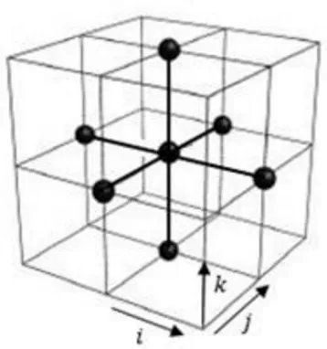
For 3D Jacobi, there has been some previous research work focusing on the optimizations on GPU platform. As shown in work [14], on GPU platform there are two types of optimization approach that can be applied on 3D Jacobi Iteration algorithms, 2.5D blocking optimization and 3D blocking optimization.

(55)

of the loaded block. The elements in the ghost layer are loaded from global memory multiple times, which will bring extra bandwidth cost. In order to minimize the amount of extra bandwidth, all the dimensions of the block are set equal to each other.

Figure 33 3D Blocking Optimization

In 2.5D blocking optimization, as shown in Figure 34 the shared memory on GPU will be allocated to perform blocking in 2D (XY) plane, and stream through the third dimension (Z). To perform computations for 3D Jacobi only 3 XY planes need to be in the buffer. Thus the total shared memory allocated is divided into three regions and each will cache an XY sub-planes. For each XY sub-plane, the computation consists of the following phases.

Phase 1: Preload - Load the next XY sub-plane into the buffer.

(56)

Phase 3: Rotation – Shift the buffered XY plane and remove the oldest XY sub-plane.

The codes to implement 2.5D blocking optimization are shown in Figure 35.

Figure 34 2.5D Blocking Optimization

(57)

better than the 3D blocking. However, the local memory resources on FPGAs are abundant compared to GPU. Also SIMD optimization could be applied directly on FPGAs design to amortize the overheads. So in this section we implement both optimizations in NDRange mode and make experiments to test if 2.5D blocking optimization outperforms 3D optimization on FPGAs.

Figure 35 2.5D Blocking Optimization Codes L0: int first=0, second=1, third=2;

L1: // pre-load the first plane

L2: src_local[first][index]=srcMatrix[first_plane_index]; L3: // pre-load the second plane

L4: src_local[second][index]=srcMatrix[second_plane_index]; L5: // perform computation through Z axis

L6: for (int k=0; k<Z_size; k++) { L7: // load the third plane

L8: src_local[third][index]=srcMatrix[first_plane_index]; L9: barrier(CLK_LOCAL_MEM_FENCE);

L10: // perform computation

L11: // store the result into external memory L12: // rotation

(58)

Figure 36 and Figure 37 present the speedup and energy consumption after applying the tuning process in the Single-Task and NDRange modes on 3D Jacobi, Table 13 and Table 14 show the corresponding resources utilization.

Figure 36 Speedups and Energy Consumption of 3D Jacobi after Applying Optimizations in the Single-Task Mode

Table 13 Resource Utilization of 3D Jacobi after Applying Optimizations in the Single-Task Mode

Naïve 26% 12% 25% 9%

SRP 19% 9% 36% 2%

SRP+TAC16 30% 14% 38% 26%

For the single-task mode, Compared to the naïve baseline kernel our optimized kernel can achieve 11.8× speedup and reduce the energy consumption from 0.09 J to 0.01 J. It can be seen from Table 13 that there are available resources for higher TAC degree. We choose TAC degree as 16 but not larger because TAC degree larger than 16 brings only slightly

2.657 J 1.722 J

0.258 J

0 2 4 6 8 10 12

Spe

(59)

higher performance (improve from 8.053 ms to 8.046 ms) but larger energy consumption (0.258 J to 0.318 J). By taking both performance and energy consumption into consideration, we decide to choose TAC degree as 16.

Figure 37 Speedups and Energy Consumption of 3D Jacobi after Applying Optimizations in the NDRange Mode

Table 14 Resource Utilization of 3D Jacobi after Applying Optimizations in the NDRange Mode

Naïve 21% 9% 19% 9%

3D

LM(16*16*16) 23% 10% 25% 7%

2.5D LM(32*32) 27% 13% 30% 8%

3D LM+SIMD8 37% 17% 29% 18%

2.5D

LM+SIMD8 51% 25% 43% 19%

9.54 J

1.903 J 1.868 J

0.872 J 0.847 J

0 2 4 6 8 10 12 14 16 Naïve 3D

LM(16*16*16) LM(32*32)2.5D 3D LM+SIMD8 LM+SIMD82.5D

Spe

(60)

In the NDRange mode, the optimized local memory size is 34x34 for 2.5D blocking optimization and 18*18*18 for 3D blocking optimization. The optimal configuration for 2.5D blocking optimization has a slightly better performance compared to the optimal configuration of 3D blocking optimization (64.407 ms vs 65.615 ms). This is because on FPGAs the only benefit which 2.5D blocking optimization take advantage of is less global memory bandwidth consumption. The local memory resources and overhead amortization are no longer problems on FPGAs. After applying the tuning process, the optimized 3D blocking optimization kernel and 2.5D blocking optimization kernel can achieve 14.7× and 14.5× speedup separately. And they reduce the energy consumption from 9.54 J to 0.872 J and 0.847 J separately.

For 3D Jacobi Iteration, compared with the optimized NDRange kernel, the optimized Single-Task kernel has better performance (8.053 ms vs 27.478 ms) and is more energy efficient. The explanation is that in Single-Task mode, the global memory accesses are consecutive, which helps to reduce the total global memory access time. And in NDRange mode, the global memory accesses are distributed among different planes, which will harm the global memory performance. Also shift registers have shorter latency and less energy consumption compared with local memory.

5.6. Comparison with Altera Design Examples

In this section, we compare our optimized kernels with the two OpenCL kernel design examples, Sobel Filter (SOBEL) and Time-Domain FIR Filter (TDFIR), provided by Altera.

(61)

processes. In the Single-Task mode, the optimized kernel for SOBEL is SRP+TAC64 (i.e., shift register optimization and task coarsening with a factor of 64), and the optimized kernel for TDFIR is SRP+TAC4. In the NDRange mode, the optimized kernel for SOBEL is LM(34*34)+LU+SIMD32 (i.e., local memory size of 34x34, loop unrolling and thread coarsening with a factor of 32), and the optimized kernel for TDFIR is LM(160)+LU+SIMD4. Figure 38 shows the speedup and energy consumption of our optimized kernels compared with the kernels provided by Altera. From the figure we can see our optimized Singe-Task kernels can achieve a speedup 7.08× and 3.45× for SOBEL and TDFIR, respectively. And the optimized NDRange kernels can achieve a speedup 3.66× and 3.33× for SOBEL and TDFIR, respectively.

Figure 38 Speedups and Energy Consumption of SOBEL and TDFIR Compared to Altera Design Examples

6. Related Work

As OpenCL for FPGAs is recently supported, there are few prior works on optimizing the OpenCL code for FGPAs. Wang et al. proposed a performance analysis framework to

0.035 J _{0.05 J}

0.006 J

0.016 J

0.013 J _{0.017 J}

0 1 2 3 4 5 6 7 8 SOBEL TDFIR Spe edup

(62)

help to optimize OpenCL codes on FPGAs [18]. The framework firstly takes an OpenCL application as an input and then performs the static statistical collection based on the corresponding LLVM IR codes as well as dynamic statistical collection by profiling the OpenCL application on GPU. The static and dynamic statistics are then fed into an analytical performance model, which will predict the corresponding performance of the OpenCL kernel. Finally the framework will also provide programmers with four metrics to indicate the current bottlenecks of the kernel. Then programmers can adjust the optimizations order or apply new optimizations based on these metrics.

(63)

7. Conclusion

(64)

REFERENCES

[1] Altera. Implementing fpga design with the opencl standard. Altera Whitepaper, 2011. [2] Altera. Altera SDK Programmer guide, 2014

[3] Altera. Altera SDK for Optimization guide, 2014.

[4] Datta, Kaushik, Mark Murphy, Vasily Volkov, Samuel Williams, Jonathan Carter, Leonid Oliker, David Patterson, John Shalf, and Katherine Yelick. "Stencil computation optimization and auto-tuning on state-of-the-art multicore architectures." In Proceedings of the 2008 ACM/IEEE conference on Supercomputing, p. 4. IEEE Press, 2008.

[5] KILL A WATT EZ. P4460 KILL A WATT EZ power meter operation manual.

http://www.p3international.com/manuals/p4460_manual.pdf.

[6] R. Fu, Haohuan, Robert G. Clapp, Oskar Mencer, and Oliver Pell. "Accelerating 3D convolution using streaming architectures on FPGAs." In 2009 SEG Annual Meeting. Society of Exploration Geophysicists, 2009.

[7] Herbordt, Martin C., Tom VanCourt, Yongfeng Gu, Bharat Sukhwani, Al Conti, Josh Model, and Doug DiSabello. "Achieving high performance with FPGA-based computing." Computer 40, no. 3 (2007): 50.

[8] Holewinski, Justin, Louis-Noël Pouchet, and Ponnuswamy Sadayappan. "High-performance code generation for stencil computations on GPU architectures." In Proceedings of the 26th ACM international conference on Supercomputing, pp. 311-320. ACM, 2012.

(65)

[10] Li, Yanhua, Youhui Zhang, Jianfeng Yang, Wayne Luk, Guangwen Yang, and Weimin Zheng. "An approach of processor core customization for stencil computation." In Application-specific Systems, Architectures and Processors (ASAP), 2014 IEEE 25th International Conference on, pp. 182-183. IEEE, 2014.

[11] Maruyama, Naoya, and Takayuki Aoki. "Optimizing stencil computations for NVIDIA Kepler GPUs." In Proceedings of the 1st International Workshop on High-Performance Stencil Computations, Vienna, pp. 89-95. 2014.

[12] Mueller, Rene, and Jens Teubner. "FPGA: what's in it for a database?." InProceedings of the 2009 ACM SIGMOD International Conference on Management of data, pp. 999-1004. ACM, 2009.

[13] Munshi, Aaftab. "The opencl specification." In 2009 IEEE Hot Chips 21 Symposium (HCS), pp. 1-314. IEEE, 2009.

[14] Nguyen, Anthony, Nadathur Satish, Jatin Chhugani, Changkyu Kim, and Pradeep Dubey. "3.5-D blocking optimization for stencil computations on modern CPUs and GPUs." In Proceedings of the 2010 ACM/IEEE International Conference for High Performance Computing, Networking, Storage and Analysis, pp. 1-13. IEEE Computer Society, 2010.

[15] Schäfer, Andreas, and Dietmar Fey. "High performance stencil code algorithms for GPGPUs." Procedia Computer Science 4 (2011): 2027-2036.

(66)

[17] Volkov, Vasily, and James W. Demmel. "Benchmarking GPUs to tune dense linear algebra." In High Performance Computing, Networking, Storage and Analysis, 2008. SC 2008. International Conference for, pp. 1-11. IEEE, 2008.

[18] Wang, Zeke, Bingsheng He, Wei Zhang, and Shunning Jiang. "A performance analysis framework for optimizing OpenCL applications on FPGAs." In 2016 IEEE International Symposium on High Performance Computer Architecture (HPCA), pp. 114-125. IEEE, 2016.