SPC based software reliability using Modified Genetic Algorithm: GO model

SPC based software reliability using Modified Genetic

Algorithm: GO model

Dr. R.Satyaprasad, U.Usha Rani, Dr. G.Krishna Mohan

Assoc.Professor, Dept. of CSE, Acharya Nagarjuna University. Research Scholar, Rayalaseema University. Professor, Dept. of CSE, KL University, Vaddeswaram.

Abstract— To assess software reliability, many software reliability growth models (SRGMs) have been proposed in the past four decades. In principle, two widely used methods for the parameter estimation of SRGMs are the maximum likelihood estimation (MLE) and the least squares estimation (LSE). However, the approach of these two estimations may impose some restrictions on SRGMs, such as the existence of derivatives from formulated models or the needs for complex calculation. In this paper, a Modified Genetic Algorithm (MGA) with Statistical Process Control (SPC) is proposed to assess the reliability of software considering the Time domain software failure data using Goel-Okumoto (GO) model which is NonHomogenous Poisson Process (NHPP) based. Experiments based on real software failure data are performed, and the results show that the proposed genetic algorithm is more effective and faster than traditional algorithms.

Keywords - Software reliability, GO model,

Time domain data, Mean Value Function,

Modified Genetic Algorithm, SPC, NHPP.

I. INTRODUCTION.

One of the most difficult problems of software

industry is to ship a reliable product. Therefore

it is necessary to have accurate and fast

estimation techniques for verifying software

reliability. Software reliability assessment is

important to evaluate the quality of software

system, since it is one of the most important

attribute of software. For Four decades, many

Software Reliability Growth Models (SRGMs)

have been proposed in estimating reliability

growth of software products. SRGMs can be

used to depict the behaviour of observed

software failures characterized by either times

of failures (i.e Time domain data) or by the

number of failures at fixed times (i.e Interval

domain data) (Lyu, 1996).

The parameters of SRGMs are generally

unknown and have to be estimated based on

collected failure data. Two of the most popular

estimation techniques are Maximum

Likelihood Estimation (MLE) and Least

Squares Estimation (LSE) (Goel, 1985; Ohba,

1984). In fact, MLE and LSE involve the

property of probability theory and statistical

analysis. Thus, this may impose some

restrictions on the parameter estimation of

Tohma, 1995) such as the continuity, the

unimodality, the existence of derivatives from

formulated models, the complex likelihood

function, etc. The method of MLE estimation

by solving a set of simultaneous equations and

is better in deriving confidence intervals. The

method of LSE minimizes the sum of squares

of the deviations between what we actually

observe and what we expect. Nevertheless,

LSE is suitable for fitting data from small to

medium sample sizes (Wood, 1996), while

MLE is considered to be better statistical

estimator for large sample sizes. In particular,

when the formulated model of SRGMs is

complicated or the sample size of failure data is

large, these two estimation techniques may not

be effective to find out the optimal solutions

and generally require to be solved numerically.

Hence, the more effective and applicable

approaches for the parameter estimation of

SRGMs may be necessary.

In recent years, the Genetic Algorithms (GAs)

has gained popularity in solving the

optimization problem of scientific fields

(Goldberg, 1989 ; Mitchell, 1998). Because,

the parameter estimation can be reformulated

as a searching process within the domain of all

the feasible solutions (Harman and Jones,

2001; Jiang, 2006), it may be attractive to

introduce GA into the process of software

reliability modeling (Dai et al., 2003). Therefore, in this paper we will propose a

modified genetic algorithm (MGA) to estimate

the parameter of the SRGMs. We will attempt

to modify GA’s operators with weighted bit

mutation and a rebuilding mechanism to

improve the performance and efficiency of

estimations. Finally, the applicability of

proposed MGA, the result of parameter

estimation and the reliability with GO model

will also be demonstrated through real data.

The rest of this paper is organized as follows.

Section 2 surveys NHPP based SRGMs and in

specific GO Model along with the past

researches of GAs in software engineering

areas. In Section 3, an effective MGA is

proposed to solve the parameter estimation of

reliability models. Then, the experimental

results based on two failure data are presented

and discussed in Section 4. Finally, some

conclusions are given in Section 5.

II. LITERATURE SURVEY.

A. NHPP model.

The Non-Homogenous Poisson Process

(NHPP) based software reliability growth

models (SRGMs) are proved to be quite

successful in practical software reliability

engineering (Musa et al., 1987). The main issue

in the NHPP model is to determine an

appropriate mean value function to denote the

expected number of failures experienced up to

a certain time point. Model parameters can be

Algorithm (MGA). Various NHPP SRGMs

have been built upon various assumptions.

Many of the SRGMs assume that each time a

failure occurs, the fault that caused it can be

immediately removed and no new faults are

introduced. Which is usually called perfect

debugging. Imperfect debugging models have

proposed a relaxation of the above assumption

(Pham, 1993).

A fault is a statement in a program which

causes one or more failures. Software

Reliability Growth is defined by the

mathematical relationship that exists between

the time span of testing a program and the

cumulative number of errors discovered. After

failure detection, we find a fault and define a

fix for the fault. The exponential software

reliability growth models are designed to

describe the failure detection process.

Let



 



software failures by time ‘t’. m(t) is the mean

value function, representing the expected

number of software failures by time ‘t’. 

 

is the failure intensity function, which is

proportional to the residual fault content. Thus

 





m t a e and

 

 

  . where

‘a’ denotes the initial number of faults

contained in a program and ‘b’ represents the

fault detection rate. In software reliability, the

initial number of faults and the fault detection

rate are always unknown. The maximum

likelihood technique can be used to evaluate

the unknown parameters. This paper deals with

the application of GO model on application test

data collected from literature, which is of Time

domain data (i.e ungrouped).

SRGMs are a statistical interpolation of defect

detection data by mathematical functions. They

have been grouped into two classes of

models-Concave and S-shaped. The only way to verify

and validate the software is by testing. This

involves running the software and checking for

unexpected behaviour of the software output

(kapur, 2009). SRGMs are used to estimate the

reliability of a software product. In literature,

we have several SRGMs developed to monitor

the reliability growth during the testing phase

of the software development. Software

reliability is defined as the probability of

failure-free software operation for specified

period of time ‘t’ in a specified environment.

B. GO Model.

The Goel-Okumoto model is a simple

Non-Homogenous Poisson Process (NHPP) model

with the mean value function

 





m t a e . Where the parameter ‘a’ is

the number of initial faults in the software and

the parameter ‘b’ is the fault detection rate. The

corresponding failure intensity function is

Assumptions:

 From the failure detection point

of view, all faults in a program are

mutually independent.

 The number of failures at any

time is proportional to the current

number of faults in a program.

 The probability of failure

detection is constant.

 The isolated faults are removed

prior to future test occasions.

C. Statistical Process Control

SPC concepts and methods are used to monitor

the performance of a software process over

time in order to verify that the process remains

in the state of statistical control. It helps in

finding assignable causes, long term

improvements in the software process.

Software quality and reliability can be achieved

by eliminating the causes or improving the

software process or its operating procedures

(Kimura, 1995).

The most popular technique for maintaining

process control is control charting. Software

process control is used to secure, that the

quality of the final product will conform to

predefined standards. In any process, regardless

of how carefully it is maintained, a certain

amount of natural variability will always exist.

A process is said to be statistically “in-control”

when it operates with only chance causes of

variation. On the other hand, when assignable

causes are present, then we say that the process

is statistically “out-of-control”. The control

charts can be classified into several categories,

according to several distinct criteria. Control

charts should be capable to create an alarm

when a shift in the level of one or more

parameters of the underlying distribution

occurs or a non-random behavior comes into.

Normally, such a situation will be reflected in

the control chart by points plotted outside the

control limits or by the presence of specific

patterns. For a process to be in control the

control chart should not have any trend or

nonrandom pattern.

SPC provides real time analysis to establish

controllable process baselines; learn, set, and

dynamically improve process capabilities; and

focus business areas needing improvement.

The early detection of software failures will

improve the software reliability. The selection

of proper SPC charts is essential to effective

statistical process control implementation and

use. The SPC chart selection is based on data,

situation and need. Many factors influence the

process, resulting in variability. The causes of

process variability can be broadly classified

into two categories, viz., assignable causes and

chance causes.

The control limits can then be utilized

to monitor the failure times of components.

the chart. If the plotted point falls between the

calculated control limits, it indicates that the

process is in the state of statistical control and

no action is warranted. If the point falls above

the UCL, it indicates that the process average,

or the failure occurrence rate, may have

decreased which resulted in an increase in the

item between failures. This is an important

indication of possible process improvement. If

this happens, the management should look for

possible causes for this improvement and if the

causes are discovered then action should be

taken to maintain them. If the plotted point falls

below the LCL, It indicates that the process

average, or the failure occurrence rate, may

have increased which resulted in a decrease in

the failure time. This means that process may

have deteriorated and thus actions should be

taken to identify and remove them.

III. MIDIFIED GENETIC

ALGORITHM.

Genetic Algorithm (GA) has been popularly

used to solve various optimization problems.

GA has advantages of easy implementation

with large search space and rapid convergence

on good quality solutions. It does not impose

restrictions on the continuity, the existence of

derivatives, and the unimodality of evaluation

functions. Traditional GA has several steps for

searching process:

 chromosome representation;

GA simulates the initial population of

parametric solution represented as

chromosomes. Each chromosome is encoded as

string of bits. Since the parameters of SRGMs

are usually real numbers, we proposed an IEEE

floating-point standard to encode

chromosomes.

Chromosome Representation and Weighted Bit Mutation

 fitness function;

Where, MSE is a measure to compare the differences between

actual values and estimators.

 Selection scheme: This scheme is to

select the candidate chromosomes from the

current population based on their fitness

values. Our goal is to maximize fitness

function for finding the best parameters.

With these fitness values, we can further

adopt roulette wheel selection and uniform

crossover to choose candidate

chromosomes. Arebuilding mechanism is

proposed. Among each generation, one best

chromosome is kept at the end of the

population to avoid disappearance from the

selection scheme. This mechanism does not

violate GA’s original purpose.

 Crossover operator: Two

chromosomes are chosen from the

population and are exchanged in part with

each other in order to improve their fitness

value. The uniform crossover is one of the

simplest forms (Goldberg, 1989). The

crossover may happen at different bits with

a probability called crossover rate, P. This

rate typically ranges from 0.5 to 0.8 from

GA literatures (Jiang, 2006). It is decide to

adopt uniform crossover in our

experiments.

 Mutation operator: In IEEE

floating-point format, it is found that some bits are

less efficient during bit mutation. The sign

bit mutation is useless as the estimated

parameter are a positive real numbers.

Similarly, if we mutate at a very high

exponential bit or at a very low fractional

bit, the whole string will respectively be

2±128 times the original or only be changed

slightly. In fact, these mutations may be too

severe or negligible. Depending on

Sensitivity analysis on different bit

mutations, a weighted bit mutation is

provided.

 Stopping criteria: The searching

process will iteratively evolve parametric

solutions until the maximal generations

equal to 10000 trials or the best fitness

function does not change in the past 10000

trials.

A. Algorithm for parameter estimation

In this section, we show how to modify the

traditional GA to estimate the parameters of

SRGMs. The detailed algorithm of MGA is

shown below. It is noted that all the proposed

mechanisms of MGA are built by using Java

programming language.

1. Initialize a population of

2. FOR (Iteration i=1;

i<=Maximum generation &&

termination condition=FALSE; i=i+1)

a.Calculate fitness for all individual

chromosomes

b. Reproduce offspring by roulette

selection

c.Choose two chromosomes from the

population in order and randomize a

probability p

d. IF p < Crossover rate THEN

i. Generate two offsprings by

recombining two chromosomes.

ENDIF

e.Choose a chromosome from the

population in order and randomize a

probability q

f.IF q < Mutation rate THEN

i. mutate the chosen chromosome at a

weighted bit position

ENDIF

g. Keep the fittest parent in the end

of population

h. Check termination condition

3. ENDFOR

4. Output estimated parameters

IV. ILLUSTRATING THE MGA.

A. Data Analysis.

There are two common types of failure data:

time-domain and interval-domain. Some

software reliability models can handle both

types of data. The time domain approach

involves recording the individual times at

which failure occurred. The interval domain

approach is characterized by counting the

number of failures occurring during a fixed

period (e.g., test session, hour, week, day). The

collected data is the Time Between Failures.

Based on the failure data collected from the

literature, we used cumulative failures data for

software reliability using GO model.

B. Distribution of Time between

failures

Based on the inter failure data given in Table 2

and 3, we compute the software failures

process through Failure Control chart. We used

cumulative time between failures data for

software reliability monitoring using GO

model. The use of cumulative quality is a

different and new approach, which is of

particular advantage in reliability.

‘a’ and ‘



b’ are Maximum Likely hood

Estimates of parameters and the values can be

computed using iterative method for the given

cumulative time between failures data. Using

‘a’ and ‘b’ values we can computem t( ).

Assuming an acceptable probability of false

alarm of 0.27%, the control limits can be

obtained as (Xie, 2002):

 

1 bt 0.99865

U

T  e 

 

1 bt 0.5

C

 

1 bt 0.00135

L

T  e 

These limits are converted to m t( )_U ,m t( )_C and

( )_L

m t form. They are used to find whether the

software process is in control or not by placing

the points in Failure control shown in figure 1

and 2 . A point below the control limit m t( )_L

indicates an alarming signal. A point above the

control limit m t( )_U indicates better quality. If

the points are falling within the control limits,

it indicates the software process is in stable

condition. The values of control limits are as

follows.

TABLE I. Estimated parameters and control limits

Data Set Parameters Control limits

a b UCL CL LCL

DS1 (NTDS) 95.382252 0.075794 95.253486 47.691126 0.128766

DS2 (IBM) 99.447446 0.019155 99.313192 49.723723 0.134254

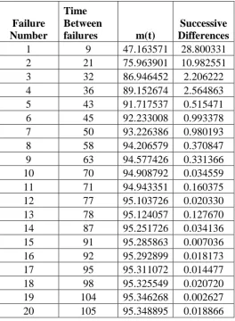
TABLE II. DS1 - Successive differences of mean value function

Failure Number

Time Between

failures m(t)

Successive Differences

1 9 47.163571 28.800331

2 21 75.963901 10.982551

3 32 86.946452 2.206222

4 36 89.152674 2.564863

5 43 91.717537 0.515471

6 45 92.233008 0.993378

7 50 93.226386 0.980193

8 58 94.206579 0.370847

9 63 94.577426 0.331366

10 70 94.908792 0.034559

11 71 94.943351 0.160375

12 77 95.103726 0.020330

13 78 95.124057 0.127670

14 87 95.251726 0.034136

15 91 95.285863 0.007036

16 92 95.292899 0.018173

17 95 95.311072 0.014477

18 98 95.325549 0.020720

19 104 95.346268 0.002627

21 116 95.367761 0.013303

22 149 95.381064 0.000489

23 156 95.381553 0.000698

24 247 95.382251 0.000000

25 249 95.382251 0.000000

26 250 95.382251

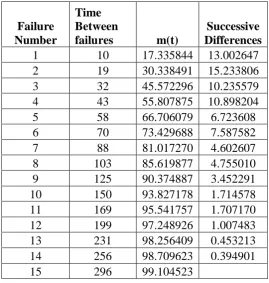
TABLE III. DS2 - Successive differences of mean value function

Failure Number

Time Between

failures m(t)

Successive Differences

1 10 17.335844 13.002647

2 19 30.338491 15.233806

3 32 45.572296 10.235579

4 43 55.807875 10.898204

5 58 66.706079 6.723608

6 70 73.429688 7.587582

7 88 81.017270 4.602607

8 103 85.619877 4.755010

9 125 90.374887 3.452291

10 150 93.827178 1.714578

11 169 95.541757 1.707170

12 199 97.248926 1.007483

13 231 98.256409 0.453213

14 256 98.709623 0.394901

Figure: 1 Failure control chart – DS1

Figure: 2 Failure control chart – DS2

V. CONCLUSION.

A number of estimates of software quality are

based on the parameter estimates of SRGMs.

Therefore, the quality estimates can be

derived based the quality estimates of

parameters. Inorder to estimate the Software

UCL_{CL 95.253485960}

47.691126021

LCL _0.128766033

0.000000 0.000000 0.000000 0.000002 0.000008 0.000031 0.000122 0.000488 0.001953 0.007813 0.031250 0.125000 0.500000 2.000000 8.000000 32.000000 128.000000

1 2 3 4 5 6 7 8 9 10 11 12 13 14 15 16 17 18 19 20 21 22 23 24 25

su

cc

es

si

ve

d

if

fe

ren

ce

s

number of inter failure time

Failure Control Chart

UCL _99.313191948

CL _49.723723022

LCL _0.134254045

0.125000 0.250000 0.500000 1.000000 2.000000 4.000000 8.000000 16.000000 32.000000 64.000000 128.000000

1 2 3 4 5 6 7 8 9 10 11 12 13 14

su

cc

es

si

ve

d

if

fe

ren

ce

s

number of inter failure time

reliability, a robust method of estimating

parameter MGA is employed on Time

domain software failure data. The graphs

have shown out of control limits i.e below the

LCL for DS1 and within control i.e between

UCL and LCL for DS2. Hence we conclude

that our method of estimation and the control

chart are giving a +ve recommendation for

their use in finding out preferable control

process or desirable out of control signal. By

observing the Failure Control chart we

identified that the failure situation is detected

at 10th point of table-1 for the corresponding

( )

m t , which is below m t( )_L . The early

detection of software failure will improve the

software Reliability. When the time between

failures is less than LCL, it is likely that there

are assignable causes leading to significant

process deterioration and it should be

investigated. On the other hand, when the

time between failures has exceeded the UCL,

there are probably reasons that have led to

significant improvement.

REFERENCES

[1] Costa, E. O., de Souza, G. A., Pozo, A.

T. R and Vergilio, S. R. (2007). "Exploring

Genetic Programming and Boosting

Techniques to Model Software Reliability,"

IEEE Transactions on Reliability, vol.56, no.

3, pp. 422-434.

[2] Dai, Y. S. Poh, K. L and Yang, B.

(2003). "Optimal Testing-Resource

Allocation with Genetic Algorithm for

Modular Software Systems," Journal of

Systems and Software, vol. 66, no. 1, pp.

47-55.

[3] Goel, A. L. (1985). "Software

Reliability Models: Assumptions,

Limitations, and Applicability," IEEE

Transactions on Software Engineering, vol.

11, no. 12, pp. 1411-1423.

[4] Goldberg, D.E. Genetic Algorithms in

Search, Optimization, and Machine Learning,

Addison-Wesley, 1989.

[5] Jiang, H. Y. (2006). "Can the Genetic

Algorithm Be a Good Tool for Software

Engineering Searching Problems?,"

Proceedings of the 30th IEEE International

Computer Software and Applications

Conference (COMPSAC 2006), pp. 362-366,

Chicago, USA.

[6] Kapur, P.K., Sunil kumar, K., Prashant,

J. Ompal, S. (2009). “Incorporating concept

of two types of imperfect debugging for

developing flexible software reliability

growth model in distributed development

environment”, Journal of Technology and

Engineering sciences, Vol.1, No.1; Jan-Jun.

[7] Kimura, M., Yamada, S., Osaki, S.,

(1995). ”Statistical Software reliability

prediction and its applicability based on mean

Computer Modelling Volume 22, Issues

10-12, Pages 149-155.

[8] Lyu, M. R. Handbook of Software

Reliability Engineering, McGraw-Hill, 1996.

[9] Harman, M and Jones, B. F. (2001).

"Search-Based Software Engineering,"

Information and Software Technology, vol.

43, no. 14, pp. 833-839.

[10] Minohara, T and Tohma, Y. (1995).

"Parameter Estimation of Hyper-Geometric

Distribution Software Reliability Growth

Model by Genetic Algorithms," Proceedings

of the 6th IEEE International Symposium on

Software Reliability Engineering (ISSRE

1995), pp. 324-329, Toulouse, France.

[11] Mitchell, M. An Introduction to Genetic

Algorithms, The MIT Press, 1998.

[12] Musa, J.D., Iannino, A., Okumoto, k.,

(1987). “Software Reliability: Measurement

Prediction Application”. McGraw-Hill, New

York.

[13] Ohba, M. (1984). "Software Reliability

Analysis Models," IBM Journal of Research

and Development, vol. 28, no. 4, pp.

428-443.

[14] Pham. H., (1993). “Software reliability

assessment: Imperfect debugging and

multiple failure types in software

development”. EG&G-RAAM10737; Idaho

National Engineering Laboratory.

[15] Wood, A. (1996). "Predicting Software

Reliability," IEEE Computer, vol. 29, no. 11,

pp. 69-77.

Authors Profile:

Dr. R. Satya Prasad received

Ph.D. degree in Computer

Science in the faculty of

Engineering in 2007 from

Acharya Nagarjuna

University, Andhra Pradesh. He received

gold medal from Acharya Nagarjuna

University for his outstanding performance in

Masters Degree. He is currently working as

Associate Professor in the Department of

Computer Science & Engineering, Acharya

Nagarjuna University. His current research is

focused on Software Engineering. He has

published 90 papers in National &

International Journals.

Mrs. U.Usha Rani,

Working as an Asst.

Professor and Head in

the Department of

Computer Science

and Engineering, Priyadarshini Engineering

College, Chintalapudi, Tenali. She obtained

her M.Sc. (Copmuter Science) degree from

KSOU, Mysore, M.Tech. (CSE) from

Acharya Nagarjuna University, Guntur. Her

research interests lies in Software

Dr. G. Krishna Mohan,

working as Professor in

the Department of

Computer Science &

Engineering, KL

University. He obtained his M.C.A degree

from Acharya Nagarjuna University,

M.Tech(CSE) from Jawaharlal Nehru

Technological University, Kakinada, M.Phil

from Madurai Kamaraj University and

Ph.D(CSE) from Acharya Nagarjuna

University. He qualified, AP State Level

Eligibility Test. His research interests lies in

Data Mining and Software Engineering. He

published 45 research papers in various