Solar PV Module Fault Analysis Using
Artificial Intelligence
Mandip Ojha1 , Prof. Nilesh Chamat 2
PG Student, Dept. of Electrical, Ballarpur Institute of Technology, Chandrapur, India 1
Assistant Professor, Dept. of Electrical, Ballarpur Institute of Technology, Chandrapur, India 2
ABSTRACT: This paper addresses the way for real time observance and fault analysis in electrical solar PV(photo
voltaic) systems is projected. This approach is based on a comparison between the performances of a faulty electrical solar PV module, with its correct model by quantifying the precise differential residue which can be associated with it. The electrical signature of each default measure mounted by considering the deformations induced on the I-V curves and PV curves. All fault cases like module to module fault, short circuit fault, open circuit fault, cell- ground faults and totally different shading patterns measure are thought-about. The projected technique measure usually generalized and extended to further forms of faults. This faults condition was analyzed by comparisons of traditional condition solar PV and VI characteristics with faulty condition characteristics. The simulation results of MATLAB simulation model shows the results for various fault condition with variation of solar irradiation
KEYWORDS: Fault analysis, solar PV module,I-V curves and PV curves, module to module fault, cell- ground faults.
I. INTRODUCTION
A PV array sometimes has multiple parallel PV strings, and every string contains a variety of modules non parallel. each module, string, and whole array, whether or not in traditional or fault condition, has its own I-V characteristics .When PV modules are connected along, their total I-V curve is set by the interactions among them. For this reason, PV modules perform together like a chain that it is only as strong as the weakest link. Faults in PV arrays damage the PV modules and cables, as well as lead to electrical shock hazards and fire risk. In this paper all fault cases like module to module fault, short circuit fault, electric circuit fault, and cell- ground faults are thought-about. Module to module fault square are the foremost common variety of fault among PV arrays. Module to module fault in PV modules occur once the electrical parameters of one module considerably modified from those of the remaining modules. This could cause irreversible damage on PV modules and huge power loss. A line-line fault is typically outlined as a short-circuit fault among PV modules or array cables with completely different potential. A short-circuit faults don't involve any ground points. . The most causes for a line-line fault could also be Incidental short between current carrying conductors, Insulation failure of cables. AN open-circuit fault is an accidental disconnection at a standard current-carrying conductor. This fault would possibly occur on cracking PV cells/modules, or between module interconnections, generally in bus wiring or junction box. Ground faults with PV modules, i.e. a photovoltaic cell short circuiting to grounded module frames because of deteriorating encapsulation of a PV module, impact damage, or water corrosion. The essential approaches of fault analysis include comparisons of traditional condition solar PV and VI characteristics with faulty condition characteristics and the simulation results of MATLAB simulation model shows the results for varied fault condition.
II. LITERATURE SURVEY
installation, such temporary fault was studied extensively in the literature (Ahmed and Salam, 2015). Wiring-related faults are common in electric circuits, there are mainly two types of faults in PV-based installations: Line-to- Ground and Line-to-Line faults. In Bower and Wiles (2000), the line-ground fault was studied only on the AC side of the PV system, whereas the authors in Stellbogen (1993), Boutasseta et al. (2013) investigated its effect on the DC side. Line-to-line fault occurs when a short-circuit between the cables of two or more PV modules with different potential is detected (Zhao et al., 2013).
To mitigate the effect of such issues, fault detection and identification (FDI) methods have been proposed to monitor the state of the PV system and warn the user of degradation signs of the PV array and any other unexpected change in the systems’ normal operation.Furthermore, FDI techniques allow the detection of wiring-related faults that may not be detected in some conditions using conventional over-current protection devices (Zhao et al., 2015). In Akram and Lotfifard (2015), a review of fault diagnosis methods on the DC side of PV arrays is given, some of the methods take into account only detection of faults and some of them make both detection and classification.In this work we consider all types of faults presented but we take into account only fault detection, as fault classification will not have much impact on the fault tolerant control algorithm.
Model-based approaches generally use an analytical model of the PV system to estimate the parameters, which will be compared to the measured ones obtained from real data. The generated residuals are used as fault features for diagnosis purposes. Recently, some model based techniques rely on the PV power losses analysis. These modeling methods need knowledge of both irradiance and PV generator temperature to predict the output power of the PV system (Chouder and Silvestre, 2010; Kang et al., 2010). More recently, model-based techniques use the empirical parameters (fill factor (ff), short-circuit current.(Isc), open-circuit voltage (Voc)…) that are calculated from the shape of the current-voltage (I-V) curves (Garoudja et al., 2017; Ali et al., 2016; Spataru et al., 2015). The main advantage of these methods is that they have low hardware requirements and are applicable to a wide range of PV systems. If the designed model can capture the main physics of the system, these methods are efficient for shading detection.Data-driven approach is based on data history, collected during operation. Fault features are extracted and analysed for fault diagnosis.
III. PROPOSED METHODOLOGY AND DISCUSSION
Mismatching fault occurs when the electrical parameters of one module are different from that of the remaining modules in a given PV installation, this fault is the most common in PV systems and may cause irreversible damage . Partial shading is a particular case of the mismatch fault, it arises when a number of PV modules are subject to a different level of solar irradiation from the rest of the installation. Wiring-related faults are common in electric circuits, there are mainly two types of faults in PV-based installations: Line-to- Ground and Line-to-Line faults.Line-to-line fault occurs when a short-circuit between the cables of two or more PV modules with different potential is detected.To mitigate the effect of such issues, fault detection and identification (FDI) methods have been proposed to monitor the state of the PV system and warn the user of degradation signs of the PV array and any other unexpected change in the systems normal operation.Furthermore, FDI techniques allow the detection of wiring-related faults that may not be detected in some conditions using conventional over-current protection devices. In this work we consider all types of faults presented but we take into account only fault detection, as fault classification will not have much impact on the fault tolerant control algorithm.
complexity in the diagnosis process development. In general, they are three main approaches used for PV fault diagnosis: image-based, model-based and process history-based also known as data-driven.The common image-based PV diagnosis methods are the ElectroLuminescence (EL) and the IRT imaging under steady state conditions. These methods are becoming increasingly popular, since they offer efficient solution not only for detecting the fault occurrence within a PV plant, but also for isolating accurately the fault. Such optical inspection techniques need appropriate and expensive equipment. ELbased diagnosis method is rather efficient to indicating the existence and the location of contact failures; cell cracks and shunts, inactive PV cells or sub- and potential induced degradation (PID) with high accuracy .
IRT-based method is fast, real time and effective to detect and exactly locate the faults thanks to the thermal signature, and without disturbing or interrupting the PV system operation. However, IRT method needs also specific conditions to be performed for correct and accurate temperature measurement. Model-based approaches generally use an analytical model of the PV system to estimate the parameters, which will be compared to the measured ones obtained from real data. The generated residuals are used as fault features for diagnosis purposes. Recently, some model based techniques rely on the PV power losses analysis
These modeling methods need knowledge of both irradiance and PV generator temperature to predict the output power of the PV system. More recently, model-based techniques use the empirical parameters that are calculated from the shape of the current-voltage (I-V) curves. The main advantage of these methods is that they have low hardware requirements and are applicable to a wide range of PV systems. If the designed model can capture the main physics of the system, these methods are efficient for shading detection.Data-driven approach is based on data history, collected during operation. Fault features are extracted and analysed for fault diagnosis. Among signal processing techniques, time-domain reflectometry (TDR) is used to detect and identify open-circuit faults and spread spectrum time-domain reflectometry (SSTDR) techniques are used to detect catastrophic faults, ground-faults and PV arc fault.
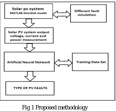
BLOCK DIAGRAM
Fig 1 Proposed methodology
IV. PROPOSED ALGORITHM
The backpropagation algorithm, is a generalization of the delta rule. If we look closely at the delta rule for single-layer
neural networks, we realize that to update a weight wik when the learning input pattern xq is presented, we need ∆wqik
= δiq.xkq
Since backpropagation uses the gradient descent method, one needs to calculate the derivative of the squared error function with respect to the weights of the network. Assuming one output neuron, the squared error function is:
, where
is the squared error,
is the target output for a training sample, and y is the actual output of the output neuron.
The factor of is included to cancel the exponent when differentiating. Later, the expression will be multiplied with an arbitrary learning rate, so that it doesn't matter if a constant coefficient is introduced now.
For each neuron , its output is defined as
.
The input to a neuron is the weighted sum of outputs of previous neurons. If the neuron is in the first layer
after the input layer, the of the input layer are simply the inputs to the network. The number of input units to
the neuron is . The variable denotes the weight between neurons and .
The activation function is in general non-linear and differentiable. A commonly used activation function is
the logistic function:
which has a nice derivative of:
1) Finding the derivative of the error
Calculating the partial derivative of the error with respect to a weight is done using the chain rule twice:
In the last term of the right-hand side, only one term in the sum depends on , so that
.
The derivative of the output of neuron with respect to its input is simply the partial derivative of the activation function (assuming here that the logistic function is used):
This is the reason why backpropagation requires the activation function to be differentiable
However, if is in an arbitrary inner layer of the network, finding the derivative with respect to is less obvious.
Considering as a function of the inputs of all neurons receiving input from neuron ,
and taking the total derivative with respect to , a recursive expression for the derivative is obtained:
Therefore, the derivative with respect to can be calculated if all the derivatives with respect to the outputs of the
next layer – the one closer to the output neuron – are known. Putting it all together:
with
To update the weight using gradient descent, one must choose a learning rate. The change in weight, which is
added to the old weight, is equal to the product of the learning rate and the gradient, multiplied by -1:
The -1 is required in order to update in the direction of a minimum, not a maximum, of the error function.
V. RESULT
Name of fault Fault case
number
Module to
ground
Module to
module
Open circuit fault
Shading effect
Mismatch fault
Module to ground 1 1 0 0 0 0
Module to module 2 0 1 0 0 0
Open circuit 3 0 0 1 0 0
Shading effect 4 0 0 0 1 0
Mismatch fault 5 0 0 0 0 1
. Table 1: Target output of ANN for solar PV module fault classification
Neural network training for solar pv system different fault classification was presented. For that separate neural network structure are utilized for classification and input for neural network was three parameters that is solar pv voltage, current and output power. The solar pv module output parameters like output voltage, output current and output power was measured at different fault conditions and that parameters was utilized for training data set for neural network training.
Neural network train for 5 types of fault conditions like module to ground, module to module, open circuit fault, and shading effect and mismatch faults. These faults conditions were simulated in matlab simulink model.
Figure ii shows the selection of percentage of training data set, validation data set and testing data set from entire 844 numbers of training samples.
Training data set: These are presented to the network during training, and the network is adjusted according to its error.
Validation data set: These are used to measure network generalization, and to halt training when generalization stops
improving.
Testing data set: These have no effect on training and so provide an independent measure of network performance during and after training.
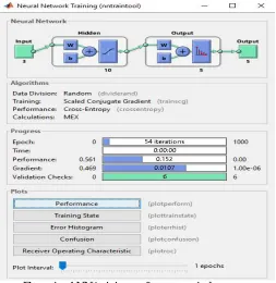
Figure iii: ANN structure during training in MATLAB Simulink
Hidden layer is consist of 10 neurons and having sigmoidal activation function of each neuron while output neuron is consist of 5 neurons and having soft competitive activation function
Figure iv: ANN training performance window
Figure iv shows the training performance window for training of pv solar system fault classification neural network. In this total 54 epochs are required for complete training of ANN using back propagation algorithm. Gradient for this
Figure v: ANN percentage error during training
Figure v shows, For training of ANN, total 488 data sample was utilized out of which 590 data set i.e. 70% data utilized for training. For validation and testing 30% dataset was utilize i.e. 127 sample data set. Also MSE (Mean square error) for all data set was 27.288 % after successful training of ANN.
Figure vi: Receiver operating characteristics for training of ANN
The receiver operating characteristic is a metric used to check the quality of classifiers. For each class of a classifier, roc applies threshold values across the interval [0,1] to outputs. For each threshold, two values are calculated, the True Positive Ratio (the number of outputs greater or equal to the threshold, divided by the number of one targets), and the
VI.CONCLUSION
Through this paper, MATLAB simulation model of solar PV array system was proposed which used to simulate different fault conditions in solar PV array system using MATLAB 2015 software. In these proposed approach different condition are simulated in which it is cleared that when open circuit fault occurs then output current an output voltage decreases very rapidly as compared with module to module and module to ground fault. Back-propogation algorithm based Neural network as artificial intelligence (AI) was utilized for classification of different solar pv fault classification. The simulation model is able to take the solar irradiance level and PV module temperature as inputs, and predict accurate steady-state performance compared with the manufacturer’s datasheet. Furthermore, the model is flexible enough to simulate solar PV arrays with different scales, with or without bypass diodes and diverse technologies. Hence this PV simulation model is modular and scalable to build PV arrays with various configurations, which is especially useful for studies of PV modules interconnection under normal and fault scenarios.
REFERENCES
1. Shen, Yanfeng; Chub, Andrii; Wang, Huai; Vinnikov, Dmitri; Liivik, Elizaveta; Blaabjerg, Frede “Wear-out Failure Analysis of an Impedance-Source PV Microinverter Based on System- Level Electrothermal Modeling ‘’Published in: I E E E Transactions on Industrial Electronics DOI (Publication date: 2019
2. Moath Alsafasfeh , Ikhlas Abdel-Qader , Bradley Bazuin , Qais Alsafasfeh , andWencong Su “Unsupervised Fault Detection and Analysis for Large Photovoltaic Systems Using Drones andb Machine Vision”Received: 25 June 2018; Accepted: 13 August 2018; Published: 27 August 2018
3. Indra Man Karmacharya, Member, IEEE, and Ramakrishna Gokaraju , Senior Member, IEEE “Fault Location in Ungrounded Photovoltaic System Using Wavelets and ANN” IEEE TRANSACTIONS ON POWER DELIVERY, VOL. 33, NO. 2, APRIL 2018
4. M. Calais, N. Wilmot, A. Ruscoe, O. Arteaga, and H. Sharma, "Over-current protection in PV array installations," presented at the ISES-AP - 3rd International Solar Energy Society Conference - Asia Pacific Region (ISES-AP-08) Sydney, 2008.
5. W. Bower and J. Wiles, "Investigation of ground-fault protection devices for photovoltaic power system applications," in Photovoltaic Specialists Conference, 2000. Conference Record of the Twenty-Eighth IEEE, pp. 1378-1383, 2000.
6. T. Esram and P. L. Chapman, "Comparison of Photovoltaic Array Maximum Power Point Tracking Techniques," Energy Conversion, IEEE Transactions on, vol. 22, pp. 439 449, 2007.
7. D. P. Hohm and M. E. Ropp, "Comparative study of maximum power point tracking algorithms using an experimental, programmable, maximum power point tracking test bed," in Photovoltaic Specialists Conference, 2000. Conference Record of the Twenty-Eighth IEEE, pp. 1699-1702, 2000.
8. VeeracharyM, "PSIM circuit-oriented simulator model for the nonlinear photovoltaic sources," Aerospace and Electronic Systems, IEEE Transactions on, vol. 42, pp. 735-740, 2006.
9. R. C. Campbell, "A Circuit-based Photovoltaic Array Model for Power System Studies," in Power Symposium, 2007. NAPS '07. 39th North American, pp. 97-101, 2007.
10. M. G. Villalva, J. R. Gazoli, and E. R. Filho, "Comprehensive Approach to Modeling and Simulation of Photovoltaic Arrays," Power Electronics, IEEE Transactions on, vol. 24, pp. 1198-1208, 2009.