Optimization of the Brillouin operator on the KNL architecture
StephanDürr1,2
1University of Wuppertal, Gaußstraße 20, D-42119 Wuppertal, Germany 2IAS/JSC, Forschungszentrum Jülich GmbH, D-52425 Jülich, Germany
Abstract.Experiences with optimizing the matrix-times-vector application of the Bril-louin operator on the Intel KNL processor are reported. Without adjustments to the mem-ory layout, performance figures of 360 Gflop/s in single and 270 Gflop/s in double pre-cision are observed. This is withNc=3 colors,Nv=12 right-hand-sides, Nthr=256
threads, on lattices of size 323×64, using exclusively OMP pragmas. Interestingly, the
same routine performs quite well on Intel Core i7 architectures, too. Some observations on the much harder Wilson fermion matrix-times-vector optimization problem are added.
1 Introduction
Conceptually the Brillouin operatorDBis a sibling of the Wilson Dirac operatorDW, since DW(x, y) =
µ
γµ∇stdµ (x, y)−
a
2std(x, y)+m0δx,y− cSW
2
µ<ν
σµνFµνδx,y (1)
DB(x, y) =
µ
γµ∇isoµ (x, y)−
a
2bri(x, y)+m0δx,y− cSW
2
µ<ν
σµνFµνδx,y (2)
share the same structure1withσ
µν=2i[γµ, γν] andFµνthe hermitean clover-leaf field-strength tensor.
The main difference is that the isotropic derivative∇isoµ and the Brillouin Laplacianbriboth include 80 neighbors (all within the [−1,+1]4hypercube around a given lattice pointx, i.e. up to 4 hops away fromx, but no two hops may be in the same direction), rather than the 8 neighbors present in the standard derivative∇stdµ and the standard Laplacianstd.
Given that the Brillouin operator has a larger “footprint” and hence more operations per site than the Wilson operator, a natural question to ask is whetherDBis more suitable for modern architectures (which typically involve lots of cores, but are limited by memory bandwidth) thanDW.
As a first step to address this question, I decided to come up with asimpleimplementation of the Brillouin operator on the Intel KNL architecture. More specifically, this boundary condition is meant to imply that (i) only shared memory parallelization via OpenMP pragmas on a single CPU is used (i.e. no distributed memory parallelization with MPI), (ii) the memory layout is unchanged from the generic layout used throughout my code suite (see below for details), and (iii) no single-thread perfor-mance tuning is attempted beyond adding straightforward SIMD hints (again via OpenMP pragmas). To the expert these constraints may look unnecessarily tight, but it turns out that nonetheless sustained performance figures2of 360 Gflop/s in single precision (sp) arithmetics can be achieved.
1m0andc
2 Brillouin operator in a nutshell
Let (λ0, λ1, λ2, λ3, λ4)≡(−240,8,4,2,1)/64; then the freebriin (2) takes the form
a2bri(x, y) = λ
0δx,y+λ1
µδx+µ,yˆ +λ2
(ν,µ)δx+µˆ+ν,yˆ
+ λ3
(ρ,ν,µ)δx+µˆ+νˆ+ρ,yˆ +λ4
(σ,ρ,ν,µ)δx+µˆ+ˆν+ρˆ+σ,yˆ (3)
where(ρ, ν, µ) means thatρ,νandµare summed over, subject to the constraint that no two elements are equal. Similarly, with (ρ1, ρ2, ρ3, ρ4)≡(64,16,4,1)/432 the free∇isoµ in (2) takes the form
a∇isoµ (x, y) = ρ1[δx+µ,yˆ −δx−µ,yˆ ]
+ ρ2
(ν;µ)[δx+µˆ+ν,yˆ −δx−µˆ+ν,yˆ ]
+ ρ3
(ρ,ν;µ)[δx+µˆ+νˆ+ρ,yˆ −δx−µˆ+νˆ+ρ,yˆ ]
+ ρ4
(σ,ρ,ν;µ)[δx+µˆ+νˆ+ρˆ+σ,yˆ −δx−µˆ+νˆ+ρˆ+σ,yˆ ] (4) where(ρ, ν;µ) means that onlyρandνare summed over, while still no two out of the three indices may be equal. In the interacting theory, these stencils are to be gauged in the obvious way. For instance, considering (3) we see 8 terms (∝λ1) with 1 hop; they are dressed withUµ(x) orUµ(x−µˆ)†,
for positive or negativeµ, respectively. Similarly, there are 24 terms with 2 hops; they are dressed with off-axis links of the form 12[Uµ(x)Uν(x+µˆ)+Uν(x)Uµ(x+νˆ)]. Next, there are 32 terms with 3
hops; they are dressed with off-axis links which are the average of 6 products of three factors each. And finally, there are 16 terms with 4 hops; they are dressed with hyperdiagonal links built as the average of 24 products of four factors each. Further details of the operator can be found in [1,2].
3 Code suite overall guidelines
The overall guidelines of the code suite are best illustrated by taking a look at the Wilson operator
DW(x, y)=12
µ
(γµ−I)Uµ(x)δx+µ,yˆ −(γµ+I)Uµ†(x−µˆ)δx−µ,yˆ
+(4+m0)δx,y (5)
which is said to operate on a vector of lengthNc4NxNyNzNt, whereNcis the number of colors.
From a computational viewpoint it is extremely convenient to declare the source and sink vectors as complex arrays of size(1:Nc,1:4,1:Nv,1:Nx*Ny*Nz*Nt). Here the ordering and the stride notation common to Matlab and Fortran are used; with the default counting from 1 we could write
(Nc,4,Nv,Nx*Ny*Nz*Nt). A special feature is that we have one slot to address the right-hand-side
(rhs), i.e.Nvcolumns (in the mathematical setup terminology) can be processed simultaneously. The
underlying philosophy is that index computations are done by the compiler, except for the site index
n=(l-1)*Nx*Ny*Nz+(k-1)*Nx*Ny+(j-1)*Nx+i, where we want to keep some freedom.
The working of these guidelines, on the basis of the Wilson operator (5), is spelled out in the code assembled in Figs.1 and2. The arrangement of the loops over the x, y,z,t coordinates (de-notedi,j,k,l, respectively) makes sure the innermost loop belongs to the fastest index. A note-worthy mathematical detail is how theNc4×Nc4 matrix 12(γµ−I)⊗Uµ(x) acts on theNc4×1 vector
old(:,:,idx,n)with given rhs and site indices. This product is realized by reshaping it into aNc×4
matrix (which it already is in our setup), multiplying it withUµ(x) from the left, and with12(γµ−I)trsp
2 Brillouin operator in a nutshell
Let (λ0, λ1, λ2, λ3, λ4)≡(−240,8,4,2,1)/64; then the freebriin (2) takes the form
a2bri(x, y) = λ
0δx,y+λ1
µδx+µ,yˆ +λ2
(ν,µ)δx+µˆ+ν,yˆ
+ λ3
(ρ,ν,µ)δx+µˆ+νˆ+ρ,yˆ +λ4
(σ,ρ,ν,µ)δx+µˆ+νˆ+ρˆ+σ,yˆ (3)
where(ρ, ν, µ) means thatρ,νandµare summed over, subject to the constraint that no two elements are equal. Similarly, with (ρ1, ρ2, ρ3, ρ4)≡(64,16,4,1)/432 the free∇isoµ in (2) takes the form
a∇isoµ (x, y) = ρ1[δx+µ,yˆ −δx−µ,yˆ ]
+ ρ2
(ν;µ)[δx+µˆ+ν,yˆ −δx−µˆ+ν,yˆ ]
+ ρ3
(ρ,ν;µ)[δx+µˆ+νˆ+ρ,yˆ −δx−µˆ+νˆ+ρ,yˆ ]
+ ρ4
(σ,ρ,ν;µ)[δx+µˆ+νˆ+ρˆ+σ,yˆ −δx−µˆ+νˆ+ρˆ+σ,yˆ ] (4) where(ρ, ν;µ) means that onlyρandνare summed over, while still no two out of the three indices may be equal. In the interacting theory, these stencils are to be gauged in the obvious way. For instance, considering (3) we see 8 terms (∝λ1) with 1 hop; they are dressed withUµ(x) orUµ(x−µˆ)†,
for positive or negativeµ, respectively. Similarly, there are 24 terms with 2 hops; they are dressed with off-axis links of the form 12[Uµ(x)Uν(x+µˆ)+Uν(x)Uµ(x+νˆ)]. Next, there are 32 terms with 3
hops; they are dressed with off-axis links which are the average of 6 products of three factors each. And finally, there are 16 terms with 4 hops; they are dressed with hyperdiagonal links built as the average of 24 products of four factors each. Further details of the operator can be found in [1,2].
3 Code suite overall guidelines
The overall guidelines of the code suite are best illustrated by taking a look at the Wilson operator
DW(x, y)=12
µ
(γµ−I)Uµ(x)δx+µ,yˆ −(γµ+I)U†µ(x−µˆ)δx−µ,yˆ
+(4+m0)δx,y (5)
which is said to operate on a vector of lengthNc4NxNyNzNt, whereNcis the number of colors.
From a computational viewpoint it is extremely convenient to declare the source and sink vectors as complex arrays of size(1:Nc,1:4,1:Nv,1:Nx*Ny*Nz*Nt). Here the ordering and the stride notation common to Matlab and Fortran are used; with the default counting from 1 we could write
(Nc,4,Nv,Nx*Ny*Nz*Nt). A special feature is that we have one slot to address the right-hand-side
(rhs), i.e.Nvcolumns (in the mathematical setup terminology) can be processed simultaneously. The
underlying philosophy is that index computations are done by the compiler, except for the site index
n=(l-1)*Nx*Ny*Nz+(k-1)*Nx*Ny+(j-1)*Nx+i, where we want to keep some freedom.
The working of these guidelines, on the basis of the Wilson operator (5), is spelled out in the code assembled in Figs.1 and 2. The arrangement of the loops over the x, y,z,t coordinates (de-notedi,j,k,l, respectively) makes sure the innermost loop belongs to the fastest index. A note-worthy mathematical detail is how theNc4×Nc4 matrix 12(γµ−I)⊗Uµ(x) acts on theNc4×1 vector
old(:,:,idx,n)with given rhs and site indices. This product is realized by reshaping it into aNc×4
matrix (which it already is in our setup), multiplying it withUµ(x) from the left, and with 12(γµ−I)trsp
from the right. The full-spinor variablefull(Nc,4)contains the result of the former multiplication; theγ-operation just reorders its columns (modulo some signs and factors of i).
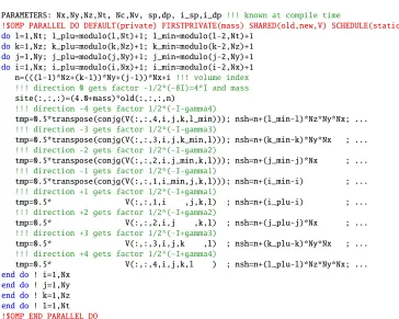
PARAMETERS: Nx,Ny,Nz,Nt, Nc,Nv, sp,dp, i_sp,i_dp !!! known at compile time
!$OMP PARALLEL DO DEFAULT(private) FIRSTPRIVATE(mass) SHARED(old,new,V) SCHEDULE(static)
dol=1,Nt; l_plu=modulo(l,Nt)+1; l_min=modulo(l-2,Nt)+1 dok=1,Nz; k_plu=modulo(k,Nz)+1; k_min=modulo(k-2,Nz)+1 doj=1,Ny; j_plu=modulo(j,Ny)+1; j_min=modulo(j-2,Ny)+1 doi=1,Nx; i_plu=modulo(i,Nx)+1; i_min=modulo(i-2,Nx)+1 n=(((l-1)*Nz+(k-1))*Ny+(j-1))*Nx+i !!! volume index !!! direction 0 gets factor -1/2*(-8I)=4*I and mass
site(:,:,:)=(4.0+mass)*old(:,:,:,n)
!!! direction -4 gets factor 1/2*(-I-gamma4)
tmp=0.5*transpose(conjg(V(:,:,4,i,j,k,l_min))); nsh=n+(l_min-l)*Nz*Ny*Nx; ...
!!! direction -3 gets factor 1/2*(-I-gamma3)
tmp=0.5*transpose(conjg(V(:,:,3,i,j,k_min,l))); nsh=n+(k_min-k)*Ny*Nx ; ...
!!! direction -2 gets factor 1/2*(-I-gamma2)
tmp=0.5*transpose(conjg(V(:,:,2,i,j_min,k,l))); nsh=n+(j_min-j)*Nx ; ...
!!! direction -1 gets factor 1/2*(-I-gamma1)
tmp=0.5*transpose(conjg(V(:,:,1,i_min,j,k,l))); nsh=n+(i_min-i) ; ...
!!! direction +1 gets factor 1/2*(-I+gamma1)
tmp=0.5* V(:,:,1,i ,j,k,l) ; nsh=n+(i_plu-i) ; ...
!!! direction +2 gets factor 1/2*(-I+gamma2)
tmp=0.5* V(:,:,2,i,j ,k,l) ; nsh=n+(j_plu-j)*Nx ; ...
!!! direction +3 gets factor 1/2*(-I+gamma3)
tmp=0.5* V(:,:,3,i,j,k ,l) ; nsh=n+(k_plu-k)*Ny*Nx ; ...
!!! direction +4 gets factor 1/2*(-I+gamma4)
tmp=0.5* V(:,:,4,i,j,k,l ) ; nsh=n+(l_plu-l)*Nz*Ny*Nx; ... end do! i=1,Nx
end do! j=1,Ny end do! k=1,Nz end do! l=1,Nt !$OMP END PARALLEL DO
Figure 1. Overall structure of the Wilson routine; accumulation of the 1+8 contributions in the thread-private variablesite(1:Nc,1:4,1:Nv)in the dotted blocks is specified in Fig.2. In the actual routineCOLLAPSE(2)
is added to the!$OMPpragma, and the the statements forl_pluandl_minare transferred to the next line.
!!! direction -1 gets factor 1/2*(-I-gamma1)
tmp=0.5*transpose(conjg(V(:,:,1,i_min,j,k,l))); nsh=n+(i_min-i) !$OMP SIMD PRIVATE(full)
doidx=1,Nv
forall(col=1:Nc,spi=1:4) full(col,spi)=sum(tmp(col,:)*old(:,spi,idx,nsh))
site(:,1,idx)=site(:,1,idx)-full(:,1)+i_sp*full(:,4) !!! gamma1^trsp= 0 0 0 i
site(:,2,idx)=site(:,2,idx)-full(:,2)+i_sp*full(:,3) !!! 0 0 i 0
site(:,3,idx)=site(:,3,idx)-full(:,3)-i_sp*full(:,2) !!! 0 -i 0 0
site(:,4,idx)=site(:,4,idx)-full(:,4)-i_sp*full(:,1) !!! -i 0 0 0
end do
!$OMP END SIMD
Figure 2.Detail of the fourth block in Fig.1; the variablefull(1:Nc,1:4)containsold(1:Nc,1:4,idx,nsh)
after left-multiplication with1
2times the link-variable, but before right-multiplication with (−I−γ1)trsp.
The name of the gauge variable in Figs.1 and2is supposed to remind us that in most practi-cal applications the smeared gauge fieldVµ(x) is used rather than the original gauge fieldUµ(x). In
case of clover improvement, it is practical to precompute the field-strength tensorFµν(x) once, and
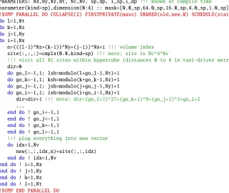
PARAMETERS: Nx,Ny,Nz,Nt, Nc,Nv, sp,dp, i_sp,i_dp !!! known at compile time
parameter(kind=sp),dimension(0:4) :: mask=[0.0_sp,64.0_sp,16.0_sp,4.0_sp,1.0_sp]/432.0_sp !$OMP PARALLEL DO COLLAPSE(2) FIRSTPRIVATE(mass) SHARED(old,new,W) SCHEDULE(static)
dol=1,Nt dok=1,Nz doj=1,Ny doi=1,Nx
n=(((l-1)*Nz+(k-1))*Ny+(j-1))*Nx+i !!! volume index
site(:,:,:)=cmplx(0.0,kind=sp) !!! note: site is Nc*4*Nv
!!! visit all 81 sites within hypercube (distances 0 to 4 in taxi-driver metric)
dir=0
do go_l=-1,1; lsh=modulo(l+go_l-1,Nt)+1 do go_k=-1,1; ksh=modulo(k+go_k-1,Nz)+1 do go_j=-1,1; jsh=modulo(j+go_j-1,Ny)+1 do go_i=-1,1; ish=modulo(i+go_i-1,Nx)+1
dir=dir+1 !!! note: dir=(go_l+1)*27+(go_k+1)*9+(go_j+1)*3+go_i+2
...
end do ! go_i=-1,1 end do ! go_j=-1,1 end do ! go_k=-1,1 end do ! go_l=-1,1
!!! plug everything into new vector
do idx=1,Nv
new(:,:,idx,n)=site(:,:,idx) end do ! idx=1,Nv
end do! i=1,Nx end do! j=1,Ny end do! k=1,Nz end do! l=1,Nt !$OMP END PARALLEL DO
Figure 3. Overall structure of the Brillouin routine; accumulation of the 81 contributions to the thread-private variablefull(1:Nc,1:4)happens in four inner loops with details specified in Fig.4.
full(:,2)-i*full(:,3)are used. Hence it would have been sufficient to form these linear
combi-nations prior to left-multiplying with the gauge field. This “shrink-expand-trick” can be used for all eight directions, regardless of theγ-representation chosen (Fig.2uses the chiral one).
4 Brillouin kernel details
The Brillouin matrix-times-vector routine, built according to the guidelines laid out in the previ-ous section, is portrayed in Figs.3and4. The four-fold loop structure over the out-vector is OMP-parallelized in the a straightforward way (theCOLLAPSE(2) statement makes sure that up toNzNt
threads can be launched). The most important difference to the Wilson routine is that 40 out of the 81 directions of the off-axis linksW, build from the smeared gauge fieldV, are assembled in the complex arrayW(Nc,Nc,40,Nx,Ny,Nz,Nt); the remaining ones are the identity or the hermitean conjugate ofWin a hypercube related point (i.e. up to four hops away).
PARAMETERS: Nx,Ny,Nz,Nt, Nc,Nv, sp,dp, i_sp,i_dp !!! known at compile time
parameter(kind=sp),dimension(0:4) :: mask=[0.0_sp,64.0_sp,16.0_sp,4.0_sp,1.0_sp]/432.0_sp !$OMP PARALLEL DO COLLAPSE(2) FIRSTPRIVATE(mass) SHARED(old,new,W) SCHEDULE(static)
do l=1,Nt do k=1,Nz do j=1,Ny do i=1,Nx
n=(((l-1)*Nz+(k-1))*Ny+(j-1))*Nx+i !!! volume index
site(:,:,:)=cmplx(0.0,kind=sp) !!! note: site is Nc*4*Nv
!!! visit all 81 sites within hypercube (distances 0 to 4 in taxi-driver metric)
dir=0
dogo_l=-1,1; lsh=modulo(l+go_l-1,Nt)+1 dogo_k=-1,1; ksh=modulo(k+go_k-1,Nz)+1 dogo_j=-1,1; jsh=modulo(j+go_j-1,Ny)+1 dogo_i=-1,1; ish=modulo(i+go_i-1,Nx)+1
dir=dir+1 !!! note: dir=(go_l+1)*27+(go_k+1)*9+(go_j+1)*3+go_i+2
...
end do! go_i=-1,1 end do! go_j=-1,1 end do! go_k=-1,1 end do! go_l=-1,1
!!! plug everything into new vector
doidx=1,Nv
new(:,:,idx,n)=site(:,:,idx) end do! idx=1,Nv
end do ! i=1,Nx end do ! j=1,Ny end do ! k=1,Nz end do ! l=1,Nt !$OMP END PARALLEL DO
Figure 3. Overall structure of the Brillouin routine; accumulation of the 81 contributions to the thread-private variablefull(1:Nc,1:4)happens in four inner loops with details specified in Fig.4.
full(:,2)-i*full(:,3)are used. Hence it would have been sufficient to form these linear
combi-nations prior to left-multiplying with the gauge field. This “shrink-expand-trick” can be used for all eight directions, regardless of theγ-representation chosen (Fig.2uses the chiral one).
4 Brillouin kernel details
The Brillouin matrix-times-vector routine, built according to the guidelines laid out in the previ-ous section, is portrayed in Figs.3and4. The four-fold loop structure over the out-vector is OMP-parallelized in the a straightforward way (theCOLLAPSE(2) statement makes sure that up to NzNt
threads can be launched). The most important difference to the Wilson routine is that 40 out of the 81 directions of the off-axis linksW, build from the smeared gauge fieldV, are assembled in the complex arrayW(Nc,Nc,40,Nx,Ny,Nz,Nt); the remaining ones are the identity or the hermitean conjugate ofWin a hypercube related point (i.e. up to four hops away).
Similar to the Wilson routine, the SIMD hints are given as pragmas to the loop over the rhs-index idx. Within this loop, the spinor and color operations are explicitly or implicitly unrolled (e.g. by forall constructs, stride notation). The complex numbers formed fromfac_i,fac_j,fac_k,fac_l implement the right-multiplication withγtrsp1 , ..., γtrsp4 in the chiral representation. All 81 contributions are accumulated in the thread-private variablesite(Nc,4,Nv); since this variable is written once to the respective site innew(:,:,:,n)there cannot be any thread-write-collision by construction.
select case(dir)
case(01:40); tmp=W(:,:,dir,i,j,k,l)
case( 41); tmp=color_eye()!!! note: yields Nc*Nc identity matrix
case(42:81); tmp=conjg(transpose(W(:,:,82-dir,ish,jsh,ksh,lsh))) end select
absgo_ijkl=sum([go_i,go_j,go_k,go_l]**2) !!! go_i**2+go_j**2+go_k**2+go_l**2
fac=0.125_sp/2**absgo_ijkl !!! note: factor for 1/2 times Brillouin Laplacian
if (absgo_ijkl.eq.0) fac=fac-2.0_sp-mass !!! note: correction for go_i=go_j=go_k=go_l=0
fac_i=go_i*mask(absgo_ijkl) !!! note: factor for isotropic derivative in x-direction
fac_j=go_j*mask(absgo_ijkl) !!! note: factor for isotropic derivative in y-direction
fac_k=go_k*mask(absgo_ijkl) !!! note: factor for isotropic derivative in z-direction
fac_l=go_l*mask(absgo_ijkl) !!! note: factor for isotropic derivative in t-direction
nsh=(((lsh-1)*Nz+(ksh-1))*Ny+(jsh-1))*Nx+ish !$OMP SIMD PRIVATE(full)
doidx=1,Nv
forall(col=1:Nc,spi=1:4) full(col,spi)=sum(tmp(col,:)*old(:,spi,idx,nsh)) site(:,:,idx)=site(:,:,idx)-fac*full(:,:)
site(:,1,idx)=site(:,1,idx)+cmplx(-fac_j,-fac_i)*full(:,4)+cmplx(+fac_l,-fac_k)*full(:,3) site(:,2,idx)=site(:,2,idx)+cmplx(+fac_j,-fac_i)*full(:,3)+cmplx(+fac_l,+fac_k)*full(:,4) site(:,3,idx)=site(:,3,idx)+cmplx(+fac_j,+fac_i)*full(:,2)+cmplx(+fac_l,+fac_k)*full(:,1) site(:,4,idx)=site(:,4,idx)+cmplx(-fac_j,+fac_i)*full(:,1)+cmplx(+fac_l,-fac_k)*full(:,2) end do! idx=1,Nv
!$OMP END SIMD
Figure 4.Detail of the dotted block in Fig.3; the variablefull(1:Nc,1:4)containsold(1:Nc,1:4,idx,nsh)
after left-multiplication with the (off-axis) link-variable, but before right-multiplication with theγ-structure.
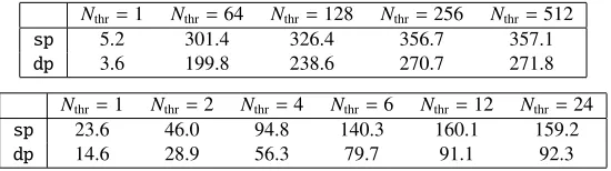
Nthr=1 Nthr=64 Nthr=128 Nthr=256 Nthr=512
sp 5.2 301.4 326.4 356.7 357.1
dp 3.6 199.8 238.6 270.7 271.8
Nthr=1 Nthr=2 Nthr=4 Nthr=6 Nthr=12 Nthr=24
sp 23.6 46.0 94.8 140.3 160.1 159.2
dp 14.6 28.9 56.3 79.7 91.1 92.3
Table 1.Performance in Gflop/s of the Brillouin matrix-times-vector operation on a 323×64 lattice, withNc=3 andNv=4Nc, versus the number of threads. The panels refer to a KNL and a Core i7 (Broadwell), respectively.
5 Brillouin operator timings
Timings are done on a node containing a single KNL chip with 64 cores. All results for the Brillouin operator are converted into Gflop/s, based on a flop count of 2560Nc2+2376Ncper site (i.e. 30168 for
QCD, see [2] for details). As a default setup we shall use a 323×64 lattice, withN
c=3 andNv=4Nc.
This geometry is chosen such that a sp-fieldW, a sp-field F, and the dp-fieldsold,newfit into the high-bandwidth MCDRAM of 16 GB. For any number of threads, memory allocation of these objects to the individual cores is done by a first-touch policy. The static thread scheduling makes sure every thread gets exactly the same fraction of theoutvector to work on. Compilation is done with ifort version 17.2, with the flags-qopenmp -O2 -xmic-avx512 -align array64byte.
10 100
1 10 100
Gflop/s [sp]
# threads
1 thread : 5.2 Gflop/s 64 threads: 301.4 Gflop/s 128 threads: 326.4 Gflop/s 256 threads: 356.7 Gflop/s
bril_sp @ KNL_64cores
10 100
1 10 100
Gflop/s [dp]
# threads
1 thread : 3.6 Gflop/s 64 threads: 199.8 Gflop/s 128 threads: 238.6 Gflop/s 256 threads: 270.7 Gflop/s
bril_dp @ KNL_64cores
Figure 5.Scaling in the number of threads of the matrix-times-vector performance of the Brillouin operator on a 323×64 lattice insp(left) anddp(right), using a KNL chip with 64 cores.
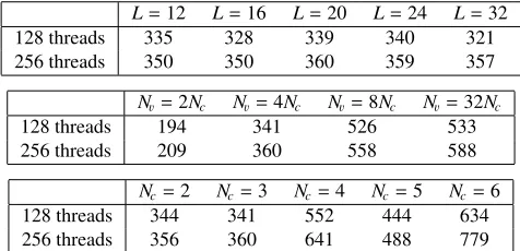
L=12 L=16 L=20 L=24 L=32
128 threads 335 328 339 340 321
256 threads 350 350 360 359 357
Nv=2Nc Nv=4Nc Nv=8Nc Nv=32Nc
128 threads 194 341 526 533
256 threads 209 360 558 588
Nc=2 Nc=3 Nc=4 Nc=5 Nc=6
128 threads 344 341 552 444 634
256 threads 356 360 641 488 779
Table 2.Performance in Gflop/s of the Brillouin matrix-times-vector operation on the KNL architecture in sp arithmetics. In the first panel the volume dependence is displayed (withNc=3,Nv=4Nc, andT =2L), in the second panel the scaling in the number of right-hand-sizes is shown (withNc=3 and 243×48 volume), and in
the third panel the dependence onNcis considered (withNv=4Ncand 243×48 volume).
Some more details are presented in Tab.1. We see some mild improvement when going from 2 to 4 threads per core; beyond 256 threads the performance plateaus. When comparing sp to dp figures, one should keep in mind that the objectsWandFare always in single precision (occupying 5760 MB and 864 MB, respectively), only the vectorsoldandnewchange from sp to dp.
Perhaps the most surprising observation is that the same routine (compiled with-xcore-avx2 instead of-xmic-avx512) performs well on a standard Core i7 architecture (Broadwell with 6 cores). Here the plateauing effect sets in after each physical core is occupied with 2 threads.
Some more experiments on the KNL architecture in sp arithmetics are reported in Tab.2. The first panel demonstrates that the∼360 Gflop/s are more or less independent of the volume, i.e. we do not see any peculiar cache size effects. The second panel shows that using more than 12 right-hand-sides (forNc = 3) improves the performance, but beyond 24 right-hand-sides benefits become marginal.
10 100
1 10 100
Gflop/s [sp]
# threads
1 thread : 5.2 Gflop/s 64 threads: 301.4 Gflop/s 128 threads: 326.4 Gflop/s 256 threads: 356.7 Gflop/s
bril_sp @ KNL_64cores
10 100
1 10 100
Gflop/s [dp]
# threads
1 thread : 3.6 Gflop/s 64 threads: 199.8 Gflop/s 128 threads: 238.6 Gflop/s 256 threads: 270.7 Gflop/s
bril_dp @ KNL_64cores
Figure 5.Scaling in the number of threads of the matrix-times-vector performance of the Brillouin operator on a 323×64 lattice insp(left) anddp(right), using a KNL chip with 64 cores.
L=12 L=16 L=20 L=24 L=32
128 threads 335 328 339 340 321
256 threads 350 350 360 359 357
Nv=2Nc Nv=4Nc Nv=8Nc Nv=32Nc
128 threads 194 341 526 533
256 threads 209 360 558 588
Nc=2 Nc=3 Nc=4 Nc=5 Nc=6
128 threads 344 341 552 444 634
256 threads 356 360 641 488 779
Table 2.Performance in Gflop/s of the Brillouin matrix-times-vector operation on the KNL architecture in sp arithmetics. In the first panel the volume dependence is displayed (withNc=3,Nv=4Nc, andT =2L), in the second panel the scaling in the number of right-hand-sizes is shown (withNc=3 and 243×48 volume), and in
the third panel the dependence onNcis considered (withNv=4Ncand 243×48 volume).
Some more details are presented in Tab.1. We see some mild improvement when going from 2 to 4 threads per core; beyond 256 threads the performance plateaus. When comparing sp to dp figures, one should keep in mind that the objectsWandFare always in single precision (occupying 5760 MB and 864 MB, respectively), only the vectorsoldandnewchange from sp to dp.
Perhaps the most surprising observation is that the same routine (compiled with-xcore-avx2 instead of-xmic-avx512) performs well on a standard Core i7 architecture (Broadwell with 6 cores). Here the plateauing effect sets in after each physical core is occupied with 2 threads.
Some more experiments on the KNL architecture in sp arithmetics are reported in Tab.2. The first panel demonstrates that the∼360 Gflop/s are more or less independent of the volume, i.e. we do not see any peculiar cache size effects. The second panel shows that using more than 12 right-hand-sides (forNc = 3) improves the performance, but beyond 24 right-hand-sides benefits become marginal.
Finally, increasing the number of colors beyond 3 is found to be particularly beneficial. My personal guess is that withNc = 4 (or a multiple thereof) the colormatrix-times-spinor multiplication in the SIMD loop in Fig.4becomes particularly efficient due to a better filling of the SIMD pipeline.
10 100
1 10 100
Gflop/s [sp]
# threads
1 thread : 2.9 Gflop/s 64 threads: 167.2 Gflop/s 128 threads: 202.9 Gflop/s 256 threads: 223.9 Gflop/s
wils_sp @ KNL_64cores
10 100
1 10 100
Gflop/s [dp]
# threads
1 thread : 2.2 Gflop/s 64 threads: 120.1 Gflop/s 128 threads: 142.5 Gflop/s 256 threads: 134.9 Gflop/s
wils_dp @ KNL_64cores
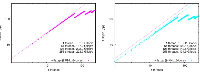
Figure 6.Scaling in the number of threads of the matrix-times-vector performance of the Wilson operator on a 323×64 lattice insp(left) anddp(right), using a KNL chip with 64 cores.
Nthr=1 Nthr=64 Nthr=128 Nthr=256 Nthr=512
sp 2.9 167.2 202.9 223.9 225.2
dp 2.2 120.1 142.5 134.9 134.2
Nthr=1 Nthr=2 Nthr=4 Nthr=6 Nthr=12 Nthr=24 sp 16.1 30.8 56.0 65.5 73.2 73.2
dp 9.8 18.0 32.5 39.9 38.7 38.6
Table 3.Performance in Gflop/s of the Wilson matrix-times-vector operation on a 323×64 lattice, withNc=3 andNv=4Nc, versus the number of threads. The panels refer to a KNL and a Core i7 (Broadwell), respectively.
6 Wilson operator timings
Timings are done on a node containing a single KNL chip with 64 cores. All results for the Wilson operator are converted into Gflop/s, based on a flop count of 128Nc2+72Ncper site (i.e. 1368 for QCD,
using the “shrink-expand-trick”, see e.g. [2] for details). The default setup is again a 323×64 lattice, withNc=3 andNv=4Nc. This time a sp-fieldV, a sp-fieldF, and the dp-fieldsold,newfit well into
the high-bandwidth MCDRAM. For any given number of threads, all arrays are allocated afresh, and a first touch policy is used as in the Brillouin case.
The scaling in the number of threads is shown in Fig.6. Again, we see a linear behavior up to 64 threads; and beyond that local maxima are seen for multiples of 64 threads where each core is kept busy with exactly the same number of threads.
KNL (64 cores) Core i7 (Broadwell) Brillouin 357/272 Gflop/s mean 6.8/10.4% 160/92 Gflop/s mean 23.2/26.7% Wilson 225/135 Gflop/s mean 4.3/5.2% 73/40 Gflop/s mean 10.6/11.6%
Table 4.Conversion of the performance measurements into sustained percentage figures, based on a peak performance of 5.2/2.6 [sp/dp] Tflop/s on the KNL and 690/345 Gflop/s on the Core i7 (Broadwell) architecture.
7 Summary
The goal of this contribution was to explore whether acceptable performance figures for the Brillouin and Wilson matrix-times-vector applications3 on one KNL chip can be obtained, if we refrain from using advanced optimization techniques (for an overview see the recent plenary talks [3,4]).
Pertinent results are summarized in Tabs.1and3 for the two operators, respectively. Not just beauty, also judgement of such figures is in the eye of the beholder. To me it appears that these are acceptable figures – especially in view of the simplicity of the shared memory parallelization and SIMD encouragement strategies used (both with OMP pragmas only).
Perhaps the most surprising finding is that these routines (unchanged, just recompiled) perform quite well on the standard Core i7 architecture, too. The loss in performance, compared to the KNL architecture, is a factor 2.2 for the Brillouin operator, and a factor 3.1 for the Wilson operator.
It is instructive to convert these figures into sustained performance ratios. The KNL chip operates at 1.269 GHz; with 64 cores and 64/32 flop/s per cycle it has a peak performance of 5.2/2.6 Tflop/s in sp/dp arithmetics. The Broadwell chip operates at 3.6 GHz; with 6 cores and 32/16 flop/s per cycle it has a peak performance of 690/345 Gflop/s in sp/dp arithmetics. With these numbers in hand, the performance figures of the Brillouin and Wilson operators can be converted into sustained performance ratios. The results, collected in Tab.4, indicate that (a) the efficiency of the Brillouin operator is generically higher than the efficiency of the Wilson operator, and (b) the efficiency on the Broadwell architecture is generically higher than the efficiency of the KNL.
An explanation of (a) is easily found. For SU(3) gauge group the Brillouin-to-Wilson flop-count ratio is 22.1. At the same time the Brillouin-to-Wilson memory-traffic ratio is 8.9 [2]. Taken together, this means that thecomputational intensityof the Brillouin operator is higher by a factor 2.5 [2]. We know that modern architectures tend to have plenty of CPU capability, and such prerequisites favor applications with high computational intensity. As for (b) the overall time (as compared to e.g. a scalar product) and the huge performance difference between SU(3) and SU(4) gauge group suggest that incomplete filling of the SIMD pipeline in theidx-loops in Figs.2 and4 likely represents the actual bottleneck (at least on the KNL architecture which operates at 512-bit width).
The main lesson is that in Lattice QCD it is easy to get a reasonable (i.e. non-excellent) perfor-mance, while maintaining full portability, if the compiler acts on code whose structure issimple4.
References
[1] S. Durr, G. Koutsou, Phys. Rev.D83, 114512 (2011),1012.3615 [2] S. Durr, G. Koutsou (2017),1701.00726
[3] P.A. Boyle,Machines and Algorithms,1702.00208
[4] A. Rago,Lattice QCD on new chips: a community summary, (these proceedings),1711.01182
![Table 4. Conversion of the performance measurements into sustained percentage figures, based on a peakperformance of 5.2/2.6 [sp/dp] Tflop/s on the KNL and 690/345 Gflop/s on the Core i7 (Broadwell) architecture.](https://thumb-us.123doks.com/thumbv2/123dok_us/8052588.1341775/8.482.80.396.78.114/conversion-performance-measurements-sustained-percentage-peakperformance-broadwell-architecture.webp)
