Shape Approximation Based on Higher-Degree Polynomials
NikolayDikusar1
1Laboratory of Information Technology, Joint Institute for Nuclear Research, Dubna, Russia
Abstract. The planar shape (contour) of an object is a fundamental source of information in a pattern recognition problem. Obtaining the relevant information set rests on difficult
procedures and is a key problem in pattern recognition. A method is proposed for the segmentation of contours with a complex geometrical form. It is based on a parametric piecewise approximation of 12th order spanned by a polynomial model defined by basic elements. Higher-order polynomial approximation allows to optimize the number of seg-ments on the contour and to obtain analytically the dependence of the curvature for more exact calculation of informative signs that are invariant to geometrical transformations. The algorithm based on this method as well as specific examples are described in detail.
1 Introduction
Not the goal is the subject of decision, but the means to the goal . . .
Aristoteles
The planar shape (contour) of the object is a fundamental source of information not only in pat-tern recognition but also in the information technologies as well. For example, to recognize objects at complex image in real time, the processor’s performance should be approximately 108–1014 elemen-tary operations per second. Therefore, instead of processing each point of the object, only its contour is processed.
Analytical curves such as pieces of straight lines, circles and spirals arches, cubic splines, etc. are used more often in the approximation of contour lines (CL). In this case the efficiency of the CL
approximation is decreased because a big number of short segments [1–3].
The goal of this work is to increase the efficiency of the pattern recognition and image processing
algorithms usinghigh-degreepolynomials for the approximation and smoothing of planar shapes. An approximation by a higher-degree polynomial has several advantages over the approximation by a low-degree polynomial. For example, if the length of intervalsincreases, the errors of the ap-proximationare decreased. The number of segments on the contouris decreased, informative signs are calculate more precisely.
The higher degree of the polynomial, the smaller the number of the grid nodes, and the accuracy and quality of the approximation is better. Increasing the degreeof the polynomialreducesthe num-ber of the nodes and improvesthe smoothness and quality of the solution inside of the interval of approximation.
At the same time, an increase in the degree of the polynomial usually leads to: loss of stabil-ity, considerable error increase of the predicted value atextrapolation,increaseof the order of the derivatives used, increaseof the computational complexity. Therefore formulas of smoothing by higher-degree polynomials are avoided almost altogether.
To reduce these difficulties, a new proposal for the choice of the polynomial spanning basis, called
the Basic Element Method (BEM) has been developed recently in our Laboratory [4–7].
A higher-order polynomial approximation allows to optimize the number of segments on the con-tour line and to obtain analytically the dependence of the curvature for it more precise calculation of informative signs that are invariant with respect to geometrical transformations.
The efficiency of the polynomial approximation and smoothing depends of many factors including
the formof the polynomial.
The new polynomial form has been constructed in the frame of BEM (BEM-polynomial). Higher-degree BEM-polynomials simplify the function approximation and data smoothing.
The following conception underlies the construction of the BEM-polynomial: “analytical con-nection between nodes of a three-point grid and corresponding triplets of pivot points of the BEM-polynomial and of its derivatives”.
2 What is a BEM-polynomial?
But very often it is important for an error to be reduced to zero within the limits of the interval[8] P. L. Chebyshev
The BEM-polynomial construction is based on Chebyshev’s idea about the approximation of a smooth function by a polynomial on an interval of limited length (1853) [8].
Thenth degree BEM-polynomial is expressed via four basic elements (BE): one cubic parabola (Q) and three quadratic parabolas (w1, w2, w3).
The four functionsQ, w1, w2, w3are defined by three nodes ofa three-point grid∆αβ3 :xα <x0<xβ and depend onτ, α, β, whereτ=x−x0,α=xα−x0,β=xβ−x0;x,xα,xβ,x0∈R.
The basic elementsw1,w2,w3 andQdepend continuously on the parametersx0,αandβ. These parameters are related to the independent variable τ by the special cross-ratio rule [ξ1ξ2ξ3ξ4] = [13]/[23] : [34]/[14], [i j] = ξj−ξi, ξj ξi. For the quadruple [ταβ0], where the first point is
fixed, this rule generates three fractional rational functionsw1,w2,w3with respect to the parameters
α,βandτ(quadratic functions relative toτ) [4]:
w1=−τ(αγτ−β), w2= τ(τβγ−α), w3= (τ−ααβ)(τ−β), γ=β−α, αβγ0, αβ <0.
The fourth elementQisa zeroingcubic parabola [4]
Q=αβτw3=τ(τ−α)(τ−β), τ, α, β∈R.
The polynomialPn(x)=ni=1aixican be written in the BEM basis form as follows:
Pn↓m(x)= m
j=0 QjΠ
j, m=n/3, m,n∈Z, (1)
At the same time, an increase in the degree of the polynomial usually leads to: loss of stabil-ity, considerable error increase of the predicted value atextrapolation,increaseof the order of the derivatives used, increase of the computational complexity. Therefore formulas of smoothing by higher-degree polynomials are avoided almost altogether.
To reduce these difficulties, a new proposal for the choice of the polynomial spanning basis, called
the Basic Element Method (BEM) has been developed recently in our Laboratory [4–7].
A higher-order polynomial approximation allows to optimize the number of segments on the con-tour line and to obtain analytically the dependence of the curvature for it more precise calculation of informative signs that are invariant with respect to geometrical transformations.
The efficiency of the polynomial approximation and smoothing depends of many factors including
the formof the polynomial.
The new polynomial form has been constructed in the frame of BEM (BEM-polynomial). Higher-degree BEM-polynomials simplify the function approximation and data smoothing.
The following conception underlies the construction of the BEM-polynomial: “analytical con-nection between nodes of a three-point grid and corresponding triplets of pivot points of the BEM-polynomial and of its derivatives”.
2 What is a BEM-polynomial?
But very often it is important for an error to be reduced to zero within the limits of the interval[8] P. L. Chebyshev
The BEM-polynomial construction is based on Chebyshev’s idea about the approximation of a smooth function by a polynomial on an interval of limited length (1853) [8].
Thenth degree BEM-polynomial is expressed via four basic elements (BE): one cubic parabola (Q) and three quadratic parabolas (w1, w2, w3).
The four functionsQ, w1, w2, w3are defined by three nodes ofa three-point grid∆αβ3 :xα<x0<xβ and depend onτ, α, β, whereτ=x−x0,α=xα−x0,β=xβ−x0;x,xα,xβ,x0 ∈R.
The basic elementsw1,w2,w3andQdepend continuously on the parametersx0,αandβ. These parameters are related to the independent variable τ by the special cross-ratio rule [ξ1ξ2ξ3ξ4] = [13]/[23] : [34]/[14], [i j] = ξj−ξi, ξj ξi. For the quadruple [ταβ0], where the first point is
fixed, this rule generates three fractional rational functionsw1,w2,w3with respect to the parameters
α,βandτ(quadratic functions relative toτ) [4]:
w1= −τ(αγτ−β), w2= τ(τβγ−α), w3= (τ−ααβ)(τ−β), γ=β−α, αβγ0, αβ <0.
The fourth elementQisa zeroingcubic parabola [4]
Q=αβτw3 =τ(τ−α)(τ−β), τ, α, β∈R.
The polynomialPn(x)=ni=1aixican be written in the BEM basis form as follows:
Pn↓m(x)= m
j=0 QjΠ
j, m=n/3, m,n∈Z, (1)
where the quadratic parabolasΠjin Eq. (1) are convolutions of the vectorw=[w1, w2, w3]Twith the vectors of the coefficientsrj=[rj1,rj2,rj3]T, i.e.Πj=wTrj, j=0,m.
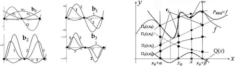
The basis functions (BF) in Eq. (1)bj(τ, α, β)=Qjwjare polynomials of the degree 3j+2 having
zeros at the nodes of the three-point grid∆αβ3 . Graphs of the BF are shown in Fig. 1, left.
The basic elements definea structureand fulfill properties such as
• natural normalizationw1+w2+w3=1;
• partial symmetrywith respect to the permutation of the parametersα↔β:
w1↔w2,w3↔w3,Q↔Q;
• scale invarianceofwj:wj(µτ, µα, µβ)=wj(τ, α, β) and • uniformityofQ:Q(µτ, µα, µβ)=µ3Q(τ, α, β).
These properties allow to optimize the parameters of a piecewise polynomial approximation (PPA) [7].
Figure 1.Graphs of the basis functions and geometric sense of thePBEM-approximation
In terms of the BF the BEM-polynomial (1) can be written as
PBEM= m
j=0 bT
jrj= m
j=0 3
i=1
bjirji, bji=Qjwi. (2)
The geometrical sense of Eq. (1) is shown in Fig. 1, right. The construction of the BEM-polynomial presents a synthesis of the properties of the Taylor polynomial and of the second degree Lagrange polynomial defined over the same three-point grid.
2.1 Properties of the BEM-Polynomials
3 Mean-Square Piecewise Polynomial Approximation Algorithm
In this section an algorithm for smoothing a planar CL is described using mean-squares piecewise BEM-polynomials of 11th degree (BEM-MSPPA).
Data smoothing using the piecewise BEM-polynomial allows to optimize the solution via the control parametersα,β,x0.The order of the derivatives is decreased substantially in comparison with the degree of the approximating polynomial in the computation ofrjν,ν=α, β,0, j=0,m [6], [7].
The algorithm BEM-MSPPA is executed in four stages: 1. An interval [a,b] and input data set{S˜} = f˜i
N
i=1 are splitted on equal (exceptKth)K N subintervals provided thatxβk−1 ≡xαk
[a,b]=kK=1[xαk,xβk], {S˜}=
K
k=1{f˜ik}
Ns
ik=1, Ns=N/K, Ns≥13. (3)
Setting parametersx0k,αk,βkandγk=βk−αkand preparation of nodes of the three-point grids:
x0k =x0k(αk, βk,Ns), xαk =x0k+αk, xβk =x0k+βk, k=1,K,
whereNsis the number of points of thekth segment on the grid∆α3kβk.
The data of each segment on the grid ∆αkβk
3 is smoothed by the 11th degree BEM-polynomial PBEM(x)=3j=0bTjrjwhere the components ofr0are pivotal points andrjis free, j=1,3 on a curve
to be approximated [4] (the indexkof the segment is dropped here and below for easy reading). 2. Calculation of ˆr0=[ ¯fα,f¯β,f0]¯ T using 2M+1 coordinates nearest the nodes of the grid∆αβ3
¯ fν= 1
2M+1 M
µ=−M
˜
fµ, ν=α, β,0; fν=f(ν)
and transformation of S-data into u-data as follows: ˜ui= f˜i−wTˆr0,i=1,Ns(see Fig. 2a).
Conditionsxβk−1≡xαk and ¯fβk−1 ≡f¯αk,k=2,KensureC0smoothness at the breakpoints.
3. Calculation of nine coefficients ˆrjusing the Least Squares Method (LSM) criterion
∂
∂rjΦ(rj)=0, where Φ(rj)= Ns
i=1 [˜ui−
3
j=1 bT
j(τi)rj]2, τi∈[α, β],
ˆ
rj=[BTB]−1BT˜u,
where˜u=[˜u1,u2˜ , . . . ,u˜Ns]T and [BTB]−1is normal matrix 9×9.
4. Estimates ˆΠj =wTjrˆj,j=1,3 are used for the calculation of ˆf(x),x∈[xα,xβ] by the Horner type scheme:
ˆ
f =Πˆ0+Q( ˆΠ1+Q( ˆΠ2+QΠˆ3)).
ˆ
u
Testings of the BEM-approximation algorithm are presented in [4]–[7]. The example in Fig. 2 shows the four stages of the BEM-MSPPA algorithm for data smoothing at the grid∆αβ3 [6].
DataS={f˜i}250i=1 was obtained by scattering points around the curve
f(x)=exp{−(x−1.3)2/[2(0.025x−0.0275)2]}+1, x∈[1.25,1.5]
using thestats[random,normald[0,0.1]](1) from a sub-package of Maple. S-data have been smoothed by the procedure
ˆ
3 Mean-Square Piecewise Polynomial Approximation Algorithm
In this section an algorithm for smoothing a planar CL is described using mean-squares piecewise BEM-polynomials of 11th degree (BEM-MSPPA).
Data smoothing using the piecewise BEM-polynomial allows to optimize the solution via the control parametersα,β,x0.The order of the derivatives is decreased substantially in comparison with the degree of the approximating polynomial in the computation ofrjν,ν=α, β,0, j=0,m [6], [7].
The algorithm BEM-MSPPA is executed in four stages: 1. An interval [a,b] and input data set{S˜} = f˜i
N
i=1 are splitted on equal (exceptKth)K N subintervals provided thatxβk−1 ≡xαk
[a,b]=kK=1[xαk,xβk], {S˜}=
K
k=1{f˜ik}
Ns
ik=1, Ns=N/K, Ns≥13. (3)
Setting parametersx0k,αk,βkandγk=βk−αkand preparation of nodes of the three-point grids:
x0k =x0k(αk, βk,Ns), xαk =x0k+αk, xβk =x0k+βk, k=1,K,
whereNsis the number of points of thekth segment on the grid∆α3kβk.
The data of each segment on the grid∆αkβk
3 is smoothed by the 11th degree BEM-polynomial PBEM(x)=3j=0bTjrjwhere the components ofr0are pivotal points andrjis free, j=1,3 on a curve
to be approximated [4] (the indexkof the segment is dropped here and below for easy reading). 2. Calculation of ˆr0=[ ¯fα,f¯β,f0]¯ T using 2M+1 coordinates nearest the nodes of the grid∆αβ3
¯ fν= 1
2M+1 M
µ=−M
˜
fµ, ν=α, β,0; fν= f(ν)
and transformation of S-data into u-data as follows: ˜ui= f˜i−wTˆr0,i=1,Ns(see Fig. 2a).
Conditionsxβk−1≡xαk and ¯fβk−1 ≡ f¯αk,k=2,KensureC0smoothness at the breakpoints.
3. Calculation of nine coefficients ˆrjusing the Least Squares Method (LSM) criterion
∂
∂rjΦ(rj)=0, where Φ(rj)= Ns
i=1 [˜ui−
3
j=1 bT
j(τi)rj]2, τi∈[α, β],
ˆ
rj=[BTB]−1BT˜u,
where˜u=[˜u1,u2˜ , . . . ,u˜Ns]T and [BTB]−1is normal matrix 9×9.
4. Estimates ˆΠj =wTjˆrj,j=1,3 are used for the calculation of ˆf(x),x∈[xα,xβ] by the Horner type scheme:
ˆ
f =Πˆ0+Q( ˆΠ1+Q( ˆΠ2+QΠˆ3)).
ˆ
u
Testings of the BEM-approximation algorithm are presented in [4]–[7]. The example in Fig. 2 shows the four stages of the BEM-MSPPA algorithm for data smoothing at the grid∆αβ3 [6].
DataS={f˜i}250i=1 was obtained by scattering points around the curve
f(x)=exp{−(x−1.3)2/[2(0.025x−0.0275)2]}+1, x∈[1.25,1.5]
using thestats[random,normald[0,0.1]](1)from a sub-package of Maple. S-data have been smoothed by the procedure
ˆ
ϕ=LeastSquares(xdat,ydat,t,curve=a_0+a_1t+...+a_{11}t^{11}).
Figure 2.Four stages of the BEM-smoothing algorithm (a) and results of the BEM-smoothing (b)
The same data have been processed by BEM-MSPPA algorithm forα = 0.025, x0 = 1.3, β = 0.05, M=7. The stages of BEM-smoothing are illustrated in Fig. 2a. 2M+1 samples are visible as
black points. Three nodes and estimates of the three pivot points ¯fα,f¯0,f¯βare marked by crosses. The graphics of Maple-estimate and BEM-estimate are denoted as ˆϕand ˆf respectively.
The deviation f − fˆis made smaller than the deviation f −ϕˆ at the expense of choosing the parameterx0in a zone of peak position (Figs. 2a, 2b).
4 Approximation of Planar Shapes
A planar CL is parametrically definable in the form of two functions x(s) and y(s) depending on a parameters(length of the arch):Γ(x(s), y(s)), s∈[0,L].
In practice, a contour line (CL) of complex topology ismeasured with errors: ˜x=x+ex,y˜=y+ey, e∼N(0, σ). BEM-MSPPA has been used for smoothing{x˜i}and{y˜i},i=1,N.
The algorithm BEM-MSPPA has five parameters for the optimization of the solution: the shift parameter (x0), three parameters oflocal smoothing(α, β,M) and one parameter ofglobal smoothing (K), where 2M+1 is the number of points nearest to the nodes of the three-point grid for the calculation
of componentsr0whileKstands for the number of segments [7].
There are hot difficulties of PPA: the optimum arrangement of the nodes on the grid and the order
of the smoothness at the breakpoints.
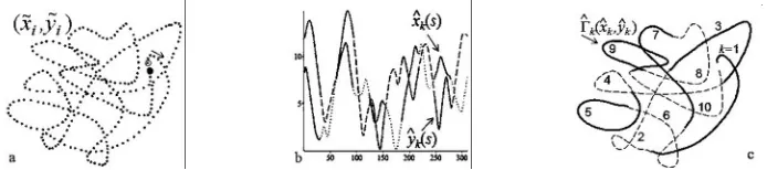
Figure 3.Parametric smoothing of a curve of complex topology using 11th degree BEM-polynomials: measure-ment points (a), estimates of ˆxkand ˆyk(b) and 10 smoothed segments (c)
The curve approximating contour of an object should lienear the measurement points, and its representation will bethe most effectiveif we usethe minimum possible number of segments K. The BEM-polynomials fulfill these requirements. The analytical dependence of the borders of complex geometric shapes is obtained through approximation (smoothing) of 2D curves.
the length of the curve has been separated by groups of three-point gridssαk ≤ s0k ≤ sβk,k=1,10:
[1,15,31],[31,46,62],[62,77,93],[93,108,124],[124,139,155],[155,170,186],[186,201,217], [217,232,248],[248,263,279],[279,294,311].
The estimates ˆxk(s), ˆyk(s),αk ≤ s ≤ sβk,k = 1,10 are 11th degree polynomials (Fig. 3b). 10
segmentsΓk( ˆxk,yˆk) are shown in Fig. 3c.
4.1 Computation of Phase Portraits and Signatures
Signature curves are very useful for developments in computer vision applications, such as artificial intelligence, medical imaging devices, the study of DNA, etc [9], [10]. Informative signs of the shape are the length of the contour lineL, the zeros of the curvatureκ(s), differential informative signs –
the phase curveΦ(κ(s), κs(s))=κ(s)/κs(s), whereκis the curvatureκ(s)= x(s)¨ +y¨(s) andκsis the
first derivative with respect to the arc length s:κs(s)=κ˙(s), etc.
Bothκandκs(as well as all higher order arc length derivatives) are Euclidean differential
invari-ants, meaning that they are unchanged under rigid motion (isometrictransformation (TI)) [11], but they change undersimilarity(TS) andaffine(TA) transformations.
It is possible to use various functions depending on the regular points (κs(s) 0) on the phase
curveΦ(κ, κs;K). To compute the signature of the shape at the nodess0k we used two values:
sgnt= 1
K
K
k=1
κ(s0k) κs(s0k)
and SGNT= 1
NT NT
i=1 sgnti,
wheres0k ∈[sαk,sβk]. SGNT is average ofNT values of sign obtained at TS- or TA- transformations.
The length of the interval [sα,sβ]increaseswiththe degree increaseof the polynomial. The inner
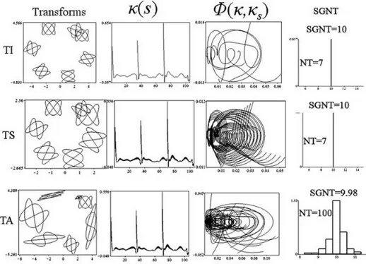
Figure 4.Graphics pointing to the change of the curvature, phase curves and histograms of SGNT under isometric (TI), similarity (TS) and affine (TA) transformations
nodess0k ∈C11will be equidistant and away from breakpoints. Thereforethe order of the smoothness
the length of the curve has been separated by groups of three-point gridssαk ≤ s0k ≤ sβk,k=1,10:
[1,15,31],[31,46,62],[62,77,93],[93,108,124],[124,139,155],[155,170,186],[186,201,217], [217,232,248],[248,263,279],[279,294,311].
The estimates ˆxk(s), ˆyk(s),αk ≤ s ≤ sβk,k = 1,10 are 11th degree polynomials (Fig. 3b). 10
segmentsΓk( ˆxk,yˆk) are shown in Fig. 3c.
4.1 Computation of Phase Portraits and Signatures
Signature curves are very useful for developments in computer vision applications, such as artificial intelligence, medical imaging devices, the study of DNA, etc [9], [10]. Informative signs of the shape are the length of the contour lineL, the zeros of the curvatureκ(s), differential informative signs –
the phase curveΦ(κ(s), κs(s))=κ(s)/κs(s), whereκis the curvatureκ(s)= x(s)¨ +y¨(s) andκsis the
first derivative with respect to the arc length s:κs(s)=κ˙(s), etc.
Bothκandκs(as well as all higher order arc length derivatives) are Euclidean differential
invari-ants, meaning that they are unchanged under rigid motion (isometrictransformation (TI)) [11], but they change undersimilarity(TS) andaffine(TA) transformations.
It is possible to use various functions depending on the regular points (κs(s) 0) on the phase
curveΦ(κ, κs;K). To compute the signature of the shape at the nodess0k we used two values:
sgnt= 1
K
K
k=1
κ(s0k) κs(s0k)
and SGNT= 1
NT NT
i=1 sgnti,
wheres0k ∈[sαk,sβk]. SGNT is average ofNT values of sign obtained at TS- or TA- transformations.
The length of the interval [sα,sβ]increaseswiththe degree increaseof the polynomial. The inner
Figure 4.Graphics pointing to the change of the curvature, phase curves and histograms of SGNT under isometric (TI), similarity (TS) and affine (TA) transformations
nodess0k ∈C11will be equidistant and away from breakpoints. Thereforethe order of the smoothness
of segments at breakpoints is not critical under such choice of the internal nodes. The request of the
second order smoothness at breakpoints is extremely important in the case of cubic splines with very short segments [2], [3].
An example of smoothing of 105 coordinates on the Lissajous figure by three BEM-polynomials of 11th degree is presented in Fig. 4. The graphics show the change of curvatures and phase curves under similarity and affine transformations of Lissajous forms. Histograms of SGNT are presented as
well. Graphics of the phase curves of 5 first segments coincide under for isometric transformations (NT =7). Fig. 5 showsNpoint data smoothing on contours of a cat (N=239) and of a dog (N=261)
respectively using the following parameters:
K = 7, M = 0, α1 = −16, β1 = 18, αk = −19, βk = 18, k = 2,7 with knots
1,35,69,103,137,171,205,239 and
K = 9, M = 0, α1 = −13, β1 = 15, αk = −16, βk = 15, k = 2,9 with knots 1,29,58,87,116,145,174,203,232,261.
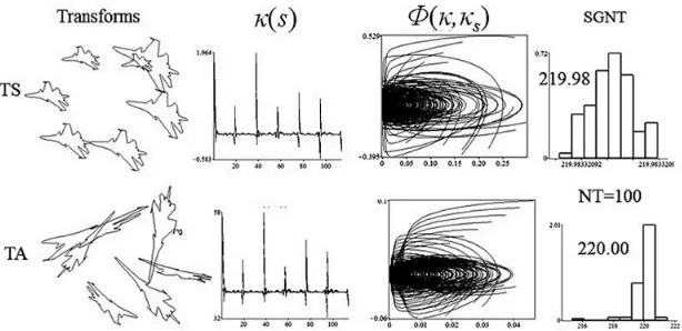
Figure 5.Measurement points, segments, phase portraits (TI,TS,TA) and SGNT computed forNT =100.
His-tograms of sign for TS and TA are shown on the right
Curvaturesκ(s) and phase portraitsΦ(κ, κs) and sign are shown in Fig. 6 under similarity and affine
transformations.
Figure 6. The curvature (first 6 segments), phase curves and histograms of sign are obtained under TS- and TA-transformations (NT=100)
The value SGNT is computed for TS and TA as average values sign obtained at NT repeated
The value SGNT is an informative sign. It can be used for objects classification, as shown in Fig. 5, where SGNTcatSGNTdog.
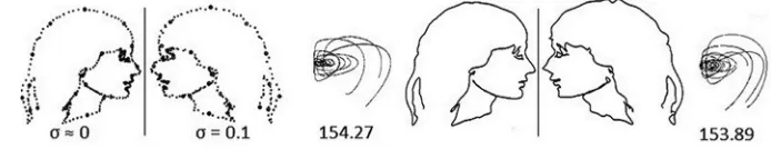
Figure 7.Mirror reflection of a face without and with errors, phase curves and SGNT
An example of BEM-segmentation of contours with errors (σ=0.1) and without (σ≈0) in input data is visualized in Fig. 7. The comparison of the phase portraits and signatures SGNT is shown for mirror reflection transformations.
5 Conclusion
In this paper, we have discussed the problem of higher-degree piecewise polynomial smoothing of digitized 1D and 2D curves and the segmentation of planar curves. A mean-squares approximation algorithm is proposed. It is spanned by a new polynomial basis, called BEM-polynomial, which is defined on a three-point grid. The construction of BEM polynomials comprises the properties of Taylor polynomial expansions around the nodes of a three-point grid and Lagrange polynomials of degree 2.
The segmentation of complex curves by cubic splines or pieces of straight lines, circles and spi-rals arches, etc. yields a big number of short segments. In comparison with these approaches, the segmentation by high-degree BEM-polynomials gives a much smaller number of segments ensuring a significantly higher order of smoothness at larger length of the interval of the three-point grid.
Examples of the segmentation of the boundary curves of objects and computations of their diff
er-ential invariant signatures confirm the efficiency of the BEM-polynomials in accuracy and quality of
approximations. The algorithm based on BEM-polynomials can be used for the classification of the contours under several geometric transformations, even in the presence of input errors.
References
[1] M. Worring,Shape Analysis of Digital Curves(Febodruk, Enschede, 1993)
[2] D. Ben-Haim, G. Harary, and A. Tal, Proceedings of the 14th ACM Symposium on Solid and Physical Modelling, 201–206, (2010)
[3] M.L. Torrente, S. Anzellotti, C. Finocchiaro, and C. Fontanari, arXiv:1507.03865v1 [math.NA] 14 Jul 2015.
[4] N.D. Dikusar, Mathematical Models and Computer Simulations3, 4, 492–507 (2011) [5] N.D. Dikusar, Mathematical Models and Computer Simulations6, 5, 509–522 (2014) [6] N.D. Dikusar, Mathematical Models and Computer Simulations8, 2, 183–200 (2016)
[7] N.D. Dikusar, http://wwwinfo.jinr.ru/publish/Preprints/2016/085(P11-2016-85).pdf [in Russian]
[8] P. L. Chebyshev,Selected Works(Akademia Nauk SSSR, Moscow, 1955), p. 639 [in Russian] [9] E. Calabi, P.J. Olver, C. Shakiban, A. Tannenbaum, and S. Haker, Int. J. Comput. Vis.26, 107–
135 (1998)
[10] M. Boutin, Int. J. Comput. Vision40(3), 235–248 (2000)