Scholarship@Western
Scholarship@Western
Electronic Thesis and Dissertation Repository
5-13-2013 12:00 AM
Localizing State-Dependent Faults Using Associated Sequence
Localizing State-Dependent Faults Using Associated Sequence
Mining
Mining
Shaimaa AliThe University of Western Ontario
Supervisor Jamie Andrews
The University of Western Ontario Graduate Program in Computer Science
A thesis submitted in partial fulfillment of the requirements for the degree in Doctor of Philosophy
© Shaimaa Ali 2013
Follow this and additional works at: https://ir.lib.uwo.ca/etd
Part of the Software Engineering Commons
Recommended Citation Recommended Citation
Ali, Shaimaa, "Localizing State-Dependent Faults Using Associated Sequence Mining" (2013). Electronic Thesis and Dissertation Repository. 1388.
https://ir.lib.uwo.ca/etd/1388
This Dissertation/Thesis is brought to you for free and open access by Scholarship@Western. It has been accepted for inclusion in Electronic Thesis and Dissertation Repository by an authorized administrator of
SEQUENCE MINING
(Thesis format: Monograph)
by
Shaimaa Ali
Graduate Program in Computer Science
A thesis submitted in partial fulfillment
of the requirements for the degree of
Doctor of Philosophy
The School of Graduate and Postdoctoral Studies
The University of Western Ontario
London, Ontario, Canada
c
In this thesis we developed a new fault localization process to localize faults in object
ori-ented software. The process is built upon the “Encapsulation” principle and aims to locate
state-dependent discrepancies in the software’s behavior. We experimented with the proposed
process on 50 seeded faults in 8 subject programs, and were able to locate the faulty class in
100% of the cases when objects with constant states were taken into consideration, while we
missed 24% percent of the faults when these objects were not considered. We also developed
a customized data mining technique “Associated sequence mining” to be used in the
localiza-tion process; experiments showed that it only provided slight enhancement to the result of the
process. The customization provided at least 17% enhancement in the time performance and
it is generic enough to be applicable in other domains. In addition to that we have developed
an extensive taxonomy for object-oriented software faults based on UML models. We used
the taxonomy to make decisions regarding the localization process.It provides an aid for
un-derstanding the nature of software faults, and will help enhance the different tasks related to
software quality assurance. The main contributions of the thesis were based on preliminary
experimentation on the usability of the classification algorithms implemented in WEKA in
software fault localization, which resulted in the conclusion that both the fault type and the
mechanism implemented in the analysis algorithm were significant to affect the results of the
localization.
Keywords: software fault localization, data mining, software faults taxonomy
Thanks to my supervisor ”Dr. Jamie Andrews”, advisors ”Dr. Nazim Madhavji” and ”Dr.
Robert Mercer” and examiners ”Dr. Hanan Lutfiyya”, ”Dr. Michael Bauer”, ”Dr. David
Bellhouse” and ”Dr. Carson Leung” for the help and advice they provided for the work in this
thesis.
Very special thanks to my parents and siblings for their support. ”I wouldn’t have done it
without you”
Thanks to my friends who gave me the social support and became like a family for me while
I’m all alone in Canada.
Many thanks to my fellow Egyptians, my fellow Muslims and my fellow humans who
supported me during my crisis without even knowing how I was. ”You have restored my faith
in humanity and I look forward to give back anonymously just like you did to me”
Abstract ii
List of Figures viii
List of Tables xi
List of Appendices xii
1 Introduction 1
1.1 Fault Localization . . . 2
1.2 Data Mining . . . 3
1.3 Thesis Contribution . . . 4
1.4 Thesis Organization . . . 5
2 Background and Related Work 6 2.1 Fault Localization . . . 6
2.1.1 Verification . . . 7
2.1.2 Checking . . . 9
2.1.3 Filtering . . . 11
2.2 Data Mining . . . 14
2.2.1 Definition . . . 14
2.2.2 The dataset to be mined . . . 14
2.2.3 The structure of the results . . . 15
2.2.4 The data mining process . . . 16
2.3 Data Mining Applied to Fault Localization . . . 21
2.4 Fault Models . . . 22
2.4.1 Definitions . . . 23
2.4.2 Orthogonal Defect Classification . . . 23
2.4.3 Comprehensive multi-dimensional taxonomy for software faults . . . . 24
Stage in the software life-cycle dimension . . . 25
Software artefact dimension . . . 26
Fault-Type dimension . . . 26
Cause dimension . . . 27
Symptoms dimension . . . 27
2.4.4 How can this multi-dimensional taxonomy be useful? . . . 27
2.4.5 UML-based fault models . . . 28
2.5 Conclusion . . . 29
3 UML-Based Fault Model 30 3.1 UML-based software faults taxonomy . . . 30
3.1.1 Structural faults . . . 31
Class structure faults . . . 31
State faults . . . 33
3.1.2 Behavioral faults . . . 33
Interaction faults . . . 35
Method implementation fault . . . 41
3.2 Which faults should we focus on? . . . 43
4 Applying an Off-the-Shelf Tool 51 4.1 The Weka Tool . . . 51
4.2 Study Design . . . 52
Concordance . . . 52
Java programs . . . 53
4.2.2 Faults . . . 53
4.2.3 Data Collection . . . 53
4.2.4 Application of Weka . . . 54
4.3 Study Results . . . 57
4.4 Summary . . . 66
5 State-Dependent Fault Localization Process and a Customized Algorithm 69 5.1 State-Dependent fault localization process . . . 69
5.2 The customized algorithm : Associated sequence mining . . . 75
5.3 FP-Growth mechanism . . . 76
5.3.1 The construction of the FP-Tree . . . 77
FP-Tree for sequential patterns . . . 84
5.3.2 Applicability to Sequential Patterns . . . 84
5.4 FP-Growth mechanism for the associated sequence mining problem . . . 85
5.4.1 The construction of the mixed FP-tree . . . 85
Algorithm 1: Construction of the mixed-FP Tree . . . 86
5.4.2 FP-growth to mine the mixed FP-tree . . . 89
Algorithm 2: FP-Growth to mine the mixed FP-Tree . . . 89
5.5 Performance Study . . . 90
5.5.1 Design . . . 90
5.5.2 Results . . . 92
5.6 Accuracy Study . . . 96
5.6.1 Subject Programs and Faults . . . 97
5.6.2 Data Collection . . . 99
5.6.3 Results . . . 102
6 Conclusion 116
6.1 Future Work . . . 117
Bibliography 118
A Numbered faults of UML-Based taxonomy 125
B Black-Box groups and values for concordance 129
Curriculum Vitae 133
1.1 Testing and debugging process . . . 2
2.1 Taxonomy of software fault localization techniques . . . 7
2.2 Verification . . . 8
2.3 Model Based Software Debugging . . . 13
2.4 Taxonomy of software fault localization techniques . . . 18
2.5 Orthogonal defect classification . . . 24
2.6 Multidimensional classification . . . 25
3.1 Structural Faults . . . 34
3.2 Interaction faults example . . . 36
3.3 Construction faults examples . . . 37
3.4 Destruction faults examples . . . 38
3.5 Sequence faults examples . . . 39
3.6 Interaction Faults . . . 40
3.7 Method Implementation Faults . . . 42
3.8 Example decision and parallelism constructs . . . 44
3.9 Forking faults examples . . . 45
3.10 Merging faults examples . . . 46
3.11 Joining faults examples . . . 47
3.12 Branching faults examples . . . 48
3.13 Branches faults examples . . . 49
3.14 Tines faults examples . . . 50
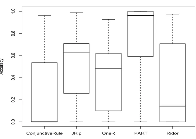
4.2 Accuracy of classifiers, all subject programs, cost sensitive data only. . . 59
4.3 Accuracy of classifiers, XML SecurityV1, cost-sensitive data only. . . 60
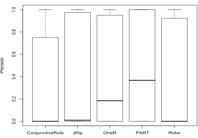
4.4 Precision of classiferies, all subject programs. . . 61
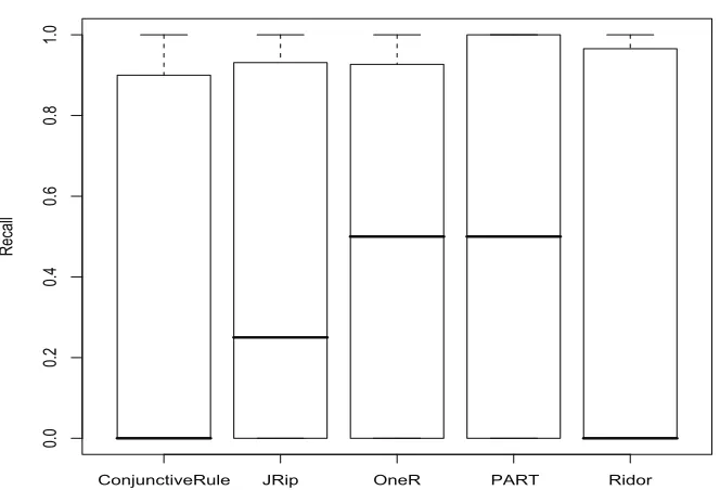
4.5 Recall of classifiers, all subject programs. . . 62
4.6 Recall of classifiers, all subject programs, cost-sensitive data only. . . 63
4.7 Recall of classifiers, subject program JTopas version 1, cost-sensitive data only. 64 5.1 State-dependent faults localization process . . . 71
5.2 The FP tree after inserting T1 . . . 78
5.3 The FP tree after inserting T1 and T2 . . . 78
5.4 The FP tree after inserting transactions up to T14 . . . 79
5.5 The FP tree after inserting transactions up to T19 . . . 79
5.6 The FP tree after inserting transactions up to T11 . . . 80
5.7 The FP tree with the order relationships preserved . . . 81
5.8 Mixed FP tree . . . 82
5.9 Time taken to build the FP trees in experiment 1 . . . 93
5.10 Time taken for mining the FP trees in experiment 1 . . . 94
5.11 Overall time taken for buliding and mining the FP trees in experiment 1 . . . . 95
5.12 Time taken to build the FP trees in experiment 2 . . . 96
5.13 Time taken for mining the FP trees in experiment 2 . . . 97
5.14 Overall all time taken for building and mining the FP trees in experiment 2 . . . 98
5.15 Comparison betweeen the number of faults localized . . . 104
5.16 Ranks for all seeded faults with constant-state behavior taken into consideration 105 5.17 Ranks for all seeded faults with constant-state behavior not taken into consid-eration . . . 106
5.18 Sizes of suspicious lists for all seeded faults with constant-state behavior taken into consideration . . . 107
taken into consideration . . . 108
5.20 Sizes of suspicious lists for JMeterV5 seeded faults with constant-state
behav-ior taken into consideration . . . 109
5.21 Ranks for XMLSecurityV2 seeded faults with constant-state behavior taken
into consideration . . . 110
5.22 Sizes of suspicious lists for JTopasV1 seeded faults with constant-state
behav-ior not taken into consideration . . . 111
5.23 Ranks for JTopasV2 seeded faults with constant-state behavior taken into
con-sideration . . . 112
5.24 Sizes of suspicious lists for JTopasV2 seeded faults with constant-state
behav-ior not taken into consideration . . . 113
5.25 Ranks for JTopasV3 seeded faults with constant-state behavior not taken into
consideration . . . 114
4.1 Faults seeded to Concordance . . . 54
4.2 Average recall, precision and accuracy of the PART classifier, across all subject programs, under the cost-sensitive treatment. . . 65
4.3 Average recall, precision and accuracy of Weka classifiers, across all subject programs, under the cost-sensitive treatment. . . 65
4.4 Pair-wise significance of the precision . . . 67
4.5 Pair-wise significance of the accuracy . . . 68
5.1 An excerpt from the behavior log of one of the seeded faults of XML-Security V1 . . . 74
5.2 Example Dataset . . . 87
5.3 Example dataset after infrequent items removed and items reordered . . . 88
5.4 Example dataset after infrequent items removed; the order of items is kept as is 88 5.5 Mixed Dataset . . . 89
5.6 Examples of randomly generated records . . . 91
5.7 Examples of randomly generated records . . . 92
5.8 Subject Programs . . . 99
5.9 jtopas faults’ types and locations . . . 99
5.10 xml-security faults’ types and locations . . . 100
5.11 jmeter faults’ types and locations . . . 101
B.1 Black-Box groups and values for concordance . . . 132
Appendix A Numbered faults of UML-Based taxonomy . . . 125
Appendix B Black-Box groups and values for concordance . . . 129
Introduction
Maintenance is one of the most costly tasks of software engineering, especially when the
pro-gram grows in size and complexity. A central process of software maintainance is the process of
testing and debugging. The National Institution of Standards and Technology (NIST) estimated
that software errors cost the economy of the United States about $59.5 billion annually; that
amount represents about 0.6 % of the gross national product of the United States in 2002 [22].
Therefore, dealing with software errors (also known as bugs) through testing and debugging
is one of the important tasks in software development. In addition to that, previous research
indicated that approximately 50% of the cost of new systems development goes to testing and
debugging [48], let alone the cost of maintenance during the lifetime of the software.
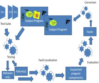
As described in Figure 1.1, the testing and debugging process starts with a subject program
that contains a number of faults, usually referred to as bugs. A test suite is prepared in order
for the testing process to begin. The result from the testing process contains the execution
behavior of each test case as well as whether it was successful or failing. This information
is then used for predicting the components of the subject program containing the faults that
caused the failures during the fault localization process. The suspected components are then
evaluated to determine whether they actually contained the fault. If so, the correction process
begins, aiming towards correcting the discovered fault(s), and the desired output is the subject
Figure 1.1: Testing and debugging process
program with a reduced number of faults in it. The scope of research of this thesis is on the
fault localization step. More specifically we are focused fault localization in object oriented
software programs.
1.1
Fault Localization
The fault localization problem is the problem of finding the location in the source code that
caused a known failure by analyzing the behavior of the program during successful and failing
test cases.
Researchers have spent a great amount of effort to automate the tasks involved in the testing
and debugging process in order to reduce the cost associated with them. One of the most
challenging tasks of the process is fault localization; i.e., after a failure has been detected, the
Unfortunately, even though some of the automated fault localization techniques are
theoret-ically very promising, they have not been practtheoret-ically used by developers. In 2011 Parnin and
Orso [45] examined whether automated software debugging is helpful for programmers. In
particular, they studied the usability of Tarantula [32] for programmers, as it is similar to most
of the state-of-the-art techniques and it was found to be the one of the most effective among
them [31]. They concluded that the programmers do not visit the ranked lines in order, and
that they prefer to have information about higher-level constructs as they can judge their
rele-vance to the failure using their names. In addition, Thung et. al [37] examined the possibility
of localizing hundreds of faults in three different Java programs, namely, AspectJ, Rhino and
Lucene. They concluded that faults are not localizable in a small number of lines, while 88%
of the faults they examined were localizable in one or two files.
1.2
Data Mining
One of the major challenges that faces fault localization techniques is the explosion of data [7].
For complex programs the amount of data that needs to be analysed to determine the faulty
component can be enormous.
As defined by [27], data mining is the analysis of large observational data sets to find
unsuspected relationships and to summarize the data in novel ways that are both understandable
and useful to the data owner; these relationships and summaries are referred to as models or
patterns.
From its definition, data mining seems to be the solution for the data explosion problem.
In addition to that, the intelligent analysis provided by data mining techniques would allow for
1.3
Thesis Contribution
We started the work on this thesis with exploratory experimentation on the usability of already
existing data mining techniques, more specifically, classification techniques implemented in
the Weka tool 1, in the problem of fault localization. We found that both the mechanism
implemented in the classification technique and the nature of the fault to be localized affected
the accuracy of the results significantly.
Combining the findings of Parnin and Orso [45] with those of Thung et al. [37] and our
initial findings, we aimed at developing a customized algorithm for fault localization that works
at the class level, that is, localizes the faulty class in object oriented software, taking the nature
of the faults to be localized in consideration.
In order to achieve that goal, we needed to understand the different types of faults that
can occur in object-oriented software. There are several taxonomies of software faults in the
literature; however, none of them provided the answer for the question we were looking at.
That is, how can we take the nature of the fault in consideration while trying to localize it?
Therefore, we created a new fault taxonomy based on the artifacts that appear in different
UML diagrams. Based on our study of the different types of faults, we decided to target one
specific type, namely, state-dependent faults, as it allows us to indirectly target the other types
as well.
Following that decision, we developed a process to collect and analyse information from
the subject program that aims at finding inconsistencies in the state-dependent behavior of that
program. We also created a customized mining algorithm that combines two existing
min-ing techniques, namely, association minmin-ing and sequence minmin-ing, that we called “associated
sequence mining”, to be used during this localization process. Finally, we evaluated both the
performance of the algorithm and the accuracy of the state-dependent fault localization process
through a set of experiments.
1.4
Thesis Organization
Chapter 2 provides the background necessary to understand the contributions of this thesis,
in addition to summarizing surveys of related work with regards to software fault localization
techniques, data mining and software fault models. Chapter 3 provides the UML-based
taxon-omy of software faults that we created to understand the nature of different faults that may occur
in object-oriented software. Chapter 4 illustrates our exploratory work using Weka classifiers
on the concordance subject program, and provides details on the results published in ASE2009
[4]. In addition, it extends that work and applies it to new Java subject programs that we used
to evaluate the new proposed technique. Chapter 5 presents the proposed state-dependent fault
localization process and the customized mining algorithm “Associated sequence mining”, in
addition to the experimental design and results for evaluating the proposals and claims made
Background and Related Work
The background of this thesis is built upon finding the answers for two main questions. What
are the existing fault localization techniques? What are the existing data mining techniques and
how can they be used for fault localization? Sections 2.1 and 2.2 provide a summary of a survey
done to find answers for these questions. During the exploratory stage of the thesis another
question came up and that was, what is it exactly that we are looking for while performing
fault localization? Therefore a survey of different software fault models and taxonomies was
performed, and is summarized in section 2.4.
2.1
Fault Localization
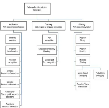
Figure 2.1 shows a taxonomy of software fault localization techniques based on their
under-lying approach. As described by Ducasse [21], software fault localization techniques can be
divided into three categories, namely Verification, Checking and Filtering. In verification, the
source code is compared to a formal specification of the program and the mismatching parts
are considered erroneous. In contrast to formal specification, checking relies on comparing the
source code to knowledge about the programming language. Finally, filtering aims at pruning
parts of the code that could not participate in the failure. More details about each of these
categories, their subcategories and some examples are provided below.
Figure 2.1: Taxonomy of software fault localization techniques
2.1.1
Verification
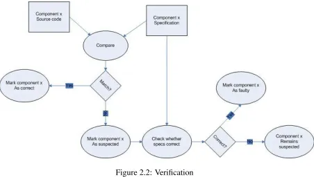
In general, the verification mechanism starts by comparing the source code and formal
spec-ifications of each component in the software under study. If the source code matches the
specifications, the component is marked correct; otherwise it is marked suspicious.
Figure 2.2: Verification
which Java APIs are detected automatically from the documentation, then used to locate faults
in client programs using those APIs while violating the specifications.
Before a final judgement is given to the component, the specification itself has to be checked
to ensure that it is correct, hence the component is erroneous. And here resides the main
disadvantage of this mechanism. Since a formal specification usually does not exist at all, and
if it exists it might be completely different than the final program, and/or it could be erroneous
in itself, the mechanism is only suitable for small (toy) programs, or as a step in a localization
process that combines different techniques.
The general steps of the verification process are shown in figure 2.2. The verification
cat-egory can be divided into seven subcategories, namely, symbolic execution, program
transfor-mation, algorithm recognition, symbolic derivation of assertions, concrete evaluation of
asser-tion, consistency checking with respect to assertions, and algorithmic behavior verification. A
brief description of each of these subcategories is mentioned below; more details are provided
by Ducasse and Emde [20].
is used to formally verify the equivalence of the model program and the actual program. For
example, Artzi et al. [6] used symbolic execution in combination with other techniques to
localize faults in PHP applications. In contrast, inprogram transformation, the model program
and the actual program are changed in parallel until either they match or diverge.
Foralgorithm recognitionthe specifications of the intended program are represented by a
set of algorithms. The implemented program then is verified against those algorithms to locate
the faulty parts. This is as opposed tosymbolic derivation of assertions, where the
specifica-tions are represented by symbolic asserspecifica-tions of program components. The specified asserspecifica-tions
are compared to corresponding symbolically derived assertions for the same component to
specify whether the implementation of that component is suspicious or not. Theconcrete
eval-uation of assertiononly differs from the preceding in that assertions are derived concretely as
opposed to symbolically.
Inconsistency checking with respect to assertions, assertions that are used to specify
prop-erties such as types, mode or dependencies are compared to the actual propprop-erties of the program
and highlight the component as suspicious if they are not consistent. Finally,algorithmic
be-havior verification assumes that the formal specifications of the whole program are present,
and the user having these specifications can act as an oracle to the verification algorithm to
compare the output of each computational step to its corresponding output in the specification.
2.1.2
Checking
The checking mechanism is similar to the verification mechanism in that it compares program
components to previous knowledge; however, the knowledge used here is specific to the
pro-gramming language as opposed to the functional formal specifications. This knowledge could
be represented as known erroneous patterns, i.e. stereotyped errors, assumed programming
conventions, or anticipated behaviour of a specific program component. Subcategories of the
checking mechanism include plan recognition, language consistency checking and stereotyped
In plan recognition, a plan is a stereotypic method of implementing a goal. In this type
of fault localization technique, the system anticipates what the programmer is trying to do
and compares it to the plan to see what went wrong. An example is what was proposed by
Johnson and Soloway [30], a system called “PROUST”. PROUST takes a Pascal program and
a non-algorithmic description of what this program should do as inputs, and then it constructs a
mapping between the two inputs using a knowledge base of programming plans and strategies
along with the bugs associated with them.
For the language consistency checking subcategory, the program is supposed to adhere
to well-formedness patterns or programming conventions. Program components are checked
against those patterns. If the code violates those patterns it is highlighted as suspicious. An
example of this approach was presented by Thummalapenta and Xie [47], who proposed a
system called “Alattin” that mines alternative acceptable patterns of conditions surrounding
Java APIs from code examples to reduce neglected conditions.
On the other hand, the approach of stereotyped error recognition is the opposite of
lan-guage consistency checking. The code is searched for known erroneous patterns which are
highlighted for further investigation. Livshits and Zimmermann [35] proposed a system called
DynaMine that combines mining (i.e. analyzing) revision history and dynamic checking. The
first is used to extract error patterns from historical records, and if any of them was discovered
in the program under study, the discovered patterns are passed to dynamic checking to verify
whether they are actually erroneous. Another use of data mining techniques for the same
pur-pose is presented by Lo et al. [36], who use feature selection to extract the program behavior
features that distinguish the faulty patterns. These features are then used in a classification
algorithm that learns which values associated with these features actually represent errors by
analyzing previous runs. The classification model is then used with new programs to locate
2.1.3
Filtering
In filtering the focus is to filter out parts of the code that do not relate to a specific error
symptom (i.e. failure), leaving the rest of the code under suspicion. Note that the objective
is not to give final judgment of the identified parts of the code, but rather point them out for
further investigation by the programmer or other techniques.
Sub-categories under filtering could be program slicing, program mutation, heuristic
filter-ing and execution trace comparison. These subcategories are described below.
The idea of the program slicing approach is to compute the statements that contribute to
calculating the value of a variable (or set of variables) at a specific point in the program. For
example, a slice that satisfies the criteria<10,x>contains all statements necessary to compute
the value of variable x at line 10 [49].
Chen and Cheung [14] illustrate the idea of program dicing, which is an additional analysis
step for the program slices. It narrows down the suspicious lines by comparing the statements
of a correct, or apparently correct, variable slice to those of an incorrect variable slice and
highlights the differences as most suspicious.
In theexecution trace comparisonapproach, execution traces of successful and failing test
runs are compared; the differences between them are highlighted as suspicious. Many of the
famous localization techniques belong to this category, including Tarantula [31], where the
suspiciousness of each statement is calculated by comparing the number of failing test cases
that execute this statement to the number of successful ones that executed it, according to the
formula
%P(s)
%P(s)+%F(s) (2.1)
where % P(s) is the percentage of passing test cases that executed the statement “s” and % F(s)
is the percentage of failing test cases that executed the statement “s”.
better results.
f(s)
p
t f ∗(f(s)+ p(s) (2.2)
where f(s) is the number of failing test cases that executed statement s, p(s) is the number of
passing test cases that executed s, and tf is the total number of failing test cases.
Zeller [51] proposed a technique to isolate cause-effect chains in a program by comparing
the values taken by each variable in a successful run by those taken in a failing one. Dallmeier
et al. [17] also proposed a comparison-based approach that compares the sequences of calls
that are more probably related to the failure. Renieris and Reiss [46] addressed the issue that
in order for the comparison approach to be successful, the compared failing and successful
runs must be quite similar; hence they proposed to choose the runs to be compared based on
a similarity measure, that is, nearest neighbor queries. Cheng et al. [15] proposed comparing
failing and successful runs after they are transformed into graphs, which are analyzed to find
the most discriminative subgraph using the graph mining algorithm LEAP.
In program mutation, small parts of the program are changed to see if the change will
cause the failure to be eliminated; if the failure still exists then the changed component is
not considered suspicious. Papadakis and Traon [44] proposed a technique of this category, in
which they calculate the suspiciousness of different mutants using the Ochiai [2] suspiciousness
measure to identify the components that are more related to the failure.
Finally, heuristic filtering involves having an a-priori hypothesis about the correctness of
some parts of the code. This can be feasible only if the hypothesis can be back-tracked. The
a-priori hypothesis can be statistical, as in the probabilistic debugging where potential faults
are calculated, and then the statements most likely to contain the errors are determined by a
belief network (e.g. Bayesian Network) [11].
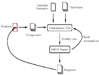
Model based software debugging is an example of the heuristic filtering approach. Model
based software debugging is the application of model-based diagnosis (MBD) used to diagnose
Figure 2.3: Model Based Software Debugging
to derive the correct behavior of the system; this behavior is then compared to the observed
behavior of the physical system. The discrepancies between the derived behavior and the
observed behavior are then used to find the diagnosis [49].
Since it is almost impossible to find a model of the correct behavior of the program, the
model here represents the actual program (containing the faults), while an oracle or test case
specifications are used to compute discrepancies between intended and actual results [49].
As Figure 2.3 illustrates, the first step in model based software debugging is to construct the
model representing the program; the model consists of the components of the program along
with relationships between them. The conformance test fails when the behavior of the program
components responsible for the conflict are computed and sent to the MBSD engine to compute
fault assumptions (i.e. variations of program expressions or components) which re-sends them
to the conformance test to be examined. At the end, the assumptions responsible for the conflict
are translated into program locations and highlighted in the source code [39].
2.2
Data Mining
In this section, we provide background about data mining, including its definition as well as the
different categories of tasks that can be performed using data mining techniques. In addition to
that, we review existing fault localization techniques that utilize these tasks.
2.2.1
Definition
As defined by Hand et. al [27], data mining is the analysis of large observational data sets to
find unsuspected relationships and to summarize the data in novel ways that are both
under-standable and useful to the data owner; these relationships and summaries are referred to as
models or patterns.
The definition implies that there are three main components: a dataset to be mined, some
desired results and a learning process for the transformation of the given dataset to the desired
results.
2.2.2
The dataset to be mined
The representation of the data
The data to be mined could be stored and represented as structured data (traditional), like most
business databases, semi-structured data, like electronic images of business documents and
medical reports, or unstructured data, like visual and multimedia recording of events. The
measure-ments (“features”, “columns”, “variables” or “dimensions”) are measured over the cases [33].
The size of the dataset
One of the factors that motivated data mining is the great amounts of data stored in databases;
these amounts of data prevented the data analysts from using them efficiently [25]. Also, large
datasets are supposed to give more valuable information since data mining can be considered
as a search through a space of possibilities; large datasets provide more possibilities to
evalu-ate [33]. Therefore data mining techniques were designed to deal with large amounts of data,
which means that applying data mining techniques on small amounts of data may yield
inac-curate results [25].
On the other hand, too large data, especially when complex analysis is needed, will cause
the analysis to be very time consuming, making such analysis impractical and infeasible. In
this case, a reduced representation of the data is obtained through applying one of the data
reduction techniques, which still maintains the integrity of the data while having a smaller size
that needs less time to be analyzed [25].
2.2.3
The structure of the results
As mentioned by Hand et al. [27], the types of the structures produced by data mining
tech-niques can be characterized by the distinction between a global model and a local pattern. A
model structure is a global summary of a dataset which makes statements on each point in the
measurement space; an example of such a model is the classifier produced by the classification
algorithm (see classification). In contrast, the pattern structure makes statements only about the
restricted regions of the space, an association rule (see dependency detection). By comparing
2.2.4
The data mining process
The main steps of the data mining process are: stating the problem, collecting the target data,
preprocessing and/or transforming the data, mining the data (applying the data mining
tech-nique), then finally interpreting the results [33], [27]. A general description of each of these
steps is given below.
Stating the problem
Since data analysis is usually associated with a certain application domain, domain-specific
knowledge and experience are usually necessary in order to come up with a meaningful
prob-lem statement. For example, in dependency detection the data analyst may specify a set of
variables for the unknown dependency and, if possible, a general form of this dependency as
an initial hypothesis. This step requires the combined expertise of the application domain and
the data mining task. In successful data mining applications, this cooperation continues during
the entire data mining process [33].
Collecting the target data
Kantardzic [33] mentioned that there are two possible approaches to collecting the data to be
mined. One of them is called “Designed Experiment”, in which the collection of data is under
the control of an expert (modeler), which results in experimental data which are collected
exclusively for analysis purposes [27]. The other approach, which is the most commonly
used, is called “the observational approach”, in which the expert cannot influence the process
of data generation, which results in “Observational data” that are collected for some other
purposes rather than data mining analysis [27]. Using observational data eliminates the effort
of applying restricted techniques for data gathering and collecting by making use of the already
existing data. On the other hand, observational data may contain missing values, noisy data or
inconsistent data, which means that data needs to be cleaned; also it is necessary to transform
Preprocessing and/or transforming the data
Generally data preprocessing may include outlier detection and removal. Outliers are odd
values in the dataset, and their existence can seriously affect the results of the data mining
technique. However, removing them may result in losing important data if these outliers did
not result from mistakes, which is the common case. The harmful effect may be avoided
using robust techniques, that are least affected by the existence of outliers. In addition the
preprocessing step may include variable scaling; for example, one feature with the range [0,
1] and the other with the range [-100, 1000] will not have the same weights in the applied
technique; they will also influence the final data-mining results differently. Therefore, it is
recommended to scale them and bring both features to the same weight for further analysis.
Also, methods for encoding and selecting features usually achieve dimensionality reduction.
In other words, they provide a smaller number of informative features for subsequent data
modeling [33].
Mining the data
Here one of the data mining tasks is performed. In general a data mining task lies in one of
four main categories: Classification, Clustering, Dependency detection and Outlier/Deviation
detection. More details on these categories are provided below.
Interpreting the results
Usually the results of data mining applications are used in decision making. Hence such results
should be interpreted in a form that is understandable by the user of these results [33]. This
Figure 2.4: Taxonomy of software fault localization techniques
2.2.5
Main categories of data mining tasks
The data mining tasks can be categorized in four different categories: classification, clustering,
association analysis and outlier detection. While the first three categories deal with knowledge
that applies to the majority of the dataset, outlier/deviation detection tries to identify the odd
(outlying) objects, as they are considered significant knowledge rather than errors or mistakes.
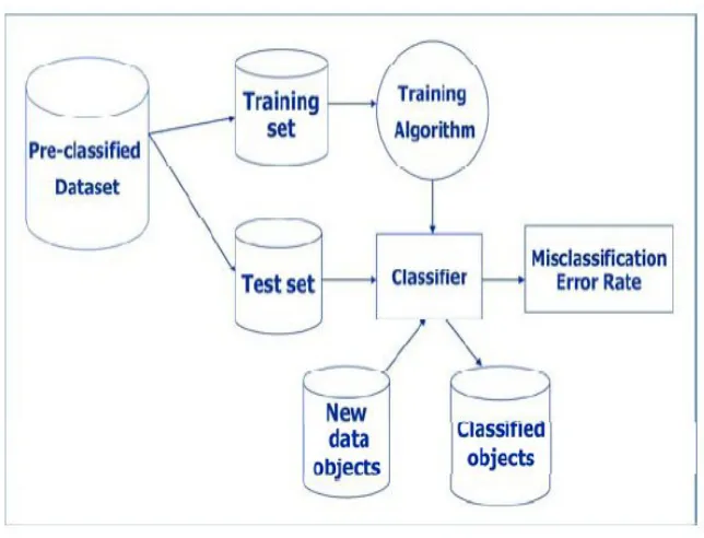
Classification
In classification the objects in the original data set are assigned to pre-specified classes (for
example, a dataset of customers is classified into buyers and non-buyers); the goal of the data
mining task is to understand the parameters affecting this assignment, and hence putting them
in a model called “the classifier”. The classifier can then be used to predict the class of a new
unclassified data object (e.g. a potential customer) with a reasonable error rate [1].
In general, the classification task is performed as illustrated in Figure 2.4. As shown in the
set, which is used by the training algorithm to generate the classifier, and the other subset is
used as a test set to evaluate the classifier; if it gives a reasonable error rate it can be used to
predict the class of new objects [1].
One of the techniques that can be used for classification is the decision tree, which can be
defined as a predictive model that can help with making complex decisions. A decision tree
may start by asking a question that has a series of answers; depending on these answers, further
questions and answers may follow. Each branch of the tree is a classification.
Clustering
In contrast to classification, the goal of the clustering task is to classify an unclassified dataset.
In clustering, groups of closely related data objects are identified; these groups may be further
analyzed to determine the characteristics of the defined groups. For example, buying habits of
multiple population segments might be compared, to determine which segments to target for a
new sales campaign [1].
Clustering analysis is performed in two main steps. The first step is to measure the
close-ness of each pair of objects in the dataset; this closeclose-ness may be expressed in terms of distances
between objects or in terms of similarities between them. The second step is to use some
clus-tering technique to identify the clusters based on the values generated in the first step.
Association Analysis
The goal of the tasks in this category is to find correlations between different items. This
correlation may be in the form of co-existence or co-occurrence; if this correlation is analyzed
on the basis of a fixed point of time, then the analysis is called Association Analysis. A typical
example of such analysis is the market basket analysis, where association rules are generated
to help in designing effective marketing campaigns and to rearrange merchandise on shelves.
To use an example that is commonly used in the literature, an association rule may indicate
association rule is a rule of the form
R:IF{AttS et1}T HEN{AttS et2}
where AttSet1 is called the antecedent and the AttSet2 is called the consequent and
AttS et1T
AttS et2=∅
For example, a typical association rule may be as follows:
IF{bread,butter}T HEN{milk}
Since a great number of rules may be produced during association analysis, there must
be some way to measure the significance of each rule. Two measures may be used for this
purpose. One of them is the support, which is the probability that a randomly chosen row
(object) from the dataset contains AttSet1; the other measure is theconfidence, which is the
conditional probability that a randomly selected object of the dataset will contain AttSet2 given
that it contains AttSet1. In terms of the support, the confidence can be calculated as shown in
Equation 2.3.
Another measure that can be used to further evaluate a rule is the lift, which can be
cal-culated as shown in Equation 2.4. Lift would indicate that the occurrence of the antecedent
increases the probability of the occurrence of the consequent in the same transaction if its value
is greater than 1, and indicates the opposite relationship if its value is less than 1. A value of 1
would indicate that there is no correlation between the two parts of the rule.
confidence(R)= support(AttS et1
S
AttS et2)
support(AttS et1) (2.3)
lift(R)= con f idence(R)
support(AttS et2) (2.4)
Another type of dependency detection is sequence-based analysis, where the co-existence
of items is analyzed on a time-interval basis, and other factors such as the order in which those
Outlier/Deviation detection
Outliers are generally the odd objects in the dataset. Outliers can be viewed from two different
perspectives: one of them considers the outliers as undesirable objects that should be treated
or deleted in the data preparation step of the data mining process, and the other considers the
outliers as interesting objects that are identified for their own interest in the data mining step of
the data mining process. In the latter case outliers should not be removed in the preprocessing
step, which is why one of the main categories of tasks performed by data mining techniques
is the outliers/deviation detection. Applications that make use of such detection include credit
card fraud detection in e-commerce applications, and network intrusion detection in the field
of network security [8].
2.3
Data Mining Applied to Fault Localization
The taxonomy of fault localization techniques shown in figure 2.1 classifies the different
tech-niques based on the underlying approach. Each of these approaches can be implemented using
different analysis techniques. Some rely on direct statistical analysis; others rely on more
complicated analysis like machine learning and data mining.
We are particularly interested in the use of data mining for fault localization. Initially we
were inspired by the work done by Denmat et al.[18] that suggested that Tarantula [31] can be
seen as an association analysis task. Tarantula as a fault localization technique is searching for
the single statements that usually cause a failure in the program when executed; this can be
reformatted into the association rule:
IF{e(s)}T HEN{F} (2.5)
That is, if a statement s is executed then probably the program fails. Tarantula’s
suspicious-ness measure can be transformed into a formula based on lift, see Equation 2.4, as shown in
S uspiciousness(s)= li f t(IF{e(s)}T HEN{F})
li f t(IF{e(s)}T HEN{S})+li f t(IF{e(s)}T HEN{F}) (2.6)
Cellier et al. [13] extended this notion to finding association rules that contain multiple lines
in the antecedant of the rule, then organizing these rules into a concept lattice in a way that helps
the programmer/debugger to identify the parts of the antecedents that are more common among
the different rules. This type of analysis still suffers from the same problem that Tarantula
suffers from, which is mainly highlighting disjoint code lines that are scattered throughout the
program, instead of highlighting higher constructs as the programmers would prefer.
Yu et al. [50] also used the task of association rule mining for fault localization; however,
their approach is to find the sequence of graphical user interface (GUI) events that led to a
failure, hence considering the event handler that most commonly called by those events as the
suspicious part of the code. Under the same category of execution trace comparison, another
mining technique is used by Cheng et al. [15] after transforming the traces into graphs and
comparing them using the graph mining algorithm LEAP. LEAP can be considered a variation
of association mining for graph data.
Furthermore, data mining can also be used in checking techniques. For example, “Alattin”,
a language consistency checking technique, also uses association mining to find acceptable
patterns of conditions surrounding Java APIs [47]. DynaMine [35] is another example of using
association mining in fault localization, which mines historical records for error patterns to be
used as stereotypes to check new code. Lo et al. [36] and Murtaza et al. [40] also proposed
using data mining for stereotyped error recognition; however, they utilized the classification
task.
2.4
Fault Models
It is crucial for software development in general and fault localization in particular to
to understand the nature of those problems starting by providing generic definitions in section
2.4.1 . The generic definitions help to provide scope to our research; however, they are not
sufficient to understand the nature of what we are looking for in fault localization, that is, the
different types of faults. Fault models provide a structure of different types of faults based on
certain criteria. In sections 2.4.2 through 2.4.5 we summarize the fault models provided in the
literature.
2.4.1
Definitions
Wieland [49] has mentioned definitions of some terms that are used to refer to problems in
software. In order to specify our focus we mention those terms and their definitions below:
Mistake: Human action that produces an incorrect result. For example copy and paste
error, spelling mistake, etc.
Failure: An incorrect result. Other sources refer to the same concept as symptom.
Error: The difference between a computed, observed, or measured value or condition and
the true, specified or theoretically correct value or condition.
Fault: An incorrect step, process or data definition. This concept is what we are focusing
on. Some sources [16] refer to it as “defect” and others refer to it as “anomaly” [41].
2.4.2
Orthogonal Defect Classification
Orthogonal Defect Classification (ODC) was developed by IBM [16] with the objective of
providing a link between the cause of the defect, represented by the associated activities of the
different stages of development, and the effect, represented in the change in the shape of the
reliability growth curve associated to a specific defect type.
As the name suggests, ODC aims at grouping software defects into classes that can be
mapped to a specific activity or stage of the development process, more like a point in a
Figure 2.5: Orthogonal defect classification
contains eight different classes of defects; each of them could be viewed as a defect either
because it is missing or because it is incorrect.
Each of the classes can be directly mapped to the stage of the process that needs the
atten-tion in order to fix the defect. The definiatten-tion of each of these classes is available in Chillarege
et al. [16].
2.4.3
Comprehensive multi-dimensional taxonomy for software faults
Inspired by the orthogonal feature of IBM’s ODC, different software fault taxonomies can be
combined in one comprehensive multi-dimensional taxonomy combining different angles of
viewing a software fault in one taxonomy.
Figure 2.6 represents the suggestion of a five-dimensional space for classifying software
Figure 2.6: Multidimensional classification
Stage in the software life-cycle dimension
This dimension might seem like “Project phase - RR200” category of IEEE’s standard
classifi-cation for software anomalies [41] recognition classificlassifi-cation scheme; however, it is different in
that this dimension represents the stage where the faults belong, while IEEE’s standard refers
to the stage where the defect/anomaly was discovered or recognized.
to the stage where the defect can be fixed, which is not necessarily the same stage where the
actual defect belongs, e.g. developer might find a detour to work around the problem instead
of directly fixing it.
The work done on Hayes’ verification and validation research project to build a
require-ments fault taxonomy for NASA [29] belongs to the requirerequire-ments part of the stages dimension.
Software artefact dimension
The artefact dimension represents the part of the software that contains the fault; including
documentation, code, underlying infrastructure (e.g. operation system), the database,
commu-nication (e.g. network topology, data transmission, etc.) and the management (e.g.plans,
pro-cedures). This is similar to IEEE’s standard classification for software anomalies [41] “Source
- IV200” criteria of classification in the investigation step. However, the same level of
granu-larity of IEEE’s standard can be achieved by specifying the corresponding value of the stage
of the software life-cycle dimension. For example, the requirements (IV211) subclass of the
specification class (IV210) corresponds to the documentation on the “artefact” dimension and
requirements on the “stages” dimension.
Similarly, the data subclass (IV217) of the specification (IV210) class corresponds to database
on the “artefact” dimension and the requirement on the “stages” dimension.
Fault-Type dimension
ODC [16] provides eight classes of defects. Some of them refer to defects in the code, e.g.
as-signment error and interface. Others refer to defects in the deployment, e.g. build/package/merge.
Finally some of them refer to defects on the functionality of the program e.g. function.
IEEE standard 1044 [41] provided eight subtypes of the type category (IV300) in the
in-vestigation classification scheme. Most of them refer to errors in the code, some refer to errors
in the data, and others refer to errors in the documentation.
classi-fying software faults focusing on faults specific to certain software architecture or feature. For
example Mariani [38] focused on the inter-component connectivity of the component-based
software while Bruning et al. [10] classified faults based on the steps of the SOA process.
Another view is based on the programming paradigm. For example, Hayes [28] provides a
taxonomy for errors specific to OOP.
Cause dimension
The term cause was used in both the ODC [16], referring to the stage of software development
that needs the attention to fix the fault, and IEEE’s standard [41], referring to the reason that
lead to the problem. The latter view is closer to our suggestion here; however, the entries that
represent the values of that dimension are quite different than classes and subclasses mentioned
in IEEE’s classification. Most of the latter were captured in the artefact dimension.
Values that can be taken on that dimension include human limitations (e.g. mis-typing),
system upgrade, bug fix (e.g. sometimes fixing a defect may cause other areas in the code to
be defective) and hardware failure.
Symptoms dimension
This dimension represents the different types of observable failures. It is similar to the symptom
category (RR500) of the recognition classification scheme of IEEE Standard [41]. Class A of
defects related to the understanding of the problem, as mentioned in Endres’ Classification of
Software Defects [12], might fit in this dimension.
The suggested multi-dimensional taxonomy can be extended by adding other dimensions
like severity (e.g. Moderate, serious, disturbing) [9] and effect on the reliability growth curve.
2.4.4
How can this multi-dimensional taxonomy be useful?
This taxonomy could be useful for researchers to determine the scope of their research; e.g. in
develop-ment stage and were found during system testing.
Also it could be useful to compare different testing and fault localization techniques in
terms of the faults they can detect or discover; hence it can realise the gaps or the areas that are
not covered by research.
In addition to that, this taxonomy can be implemented as a data warehouse to collect all
information about the different types of faults, and hence be used to facilitate the debugging
process. For example, when certain symptoms are observed, this data warehouse can be used to
find out which fault types might be associated with those symptoms and which artefact might
contain these faults.
2.4.5
UML-based fault models
Trong et al. [19] proposed a fault taxonomy for UML design models, for the objective of
being used in verification and validation of design models. The first level of the taxonomy
has three categories. One of them is for the design metrics related faults, like faults related to
cohesion and coupling. Obviously, this category is far from being related to the focus of this
thesis, as our focus is on the implemented code and faults related to it. The second is for faults
detectable without execution, which is related to faults in the syntax of the diagrams either
in a single diagram or in the consistency between different diagrams. Again, this category is
not related to the focus of this thesis as we are interested in the faults that produce failures,
i.e. run-time faults, while the faults in this category may correspond to compile time faults in
the code. Finally, the third category is for the faults related to behavior. Some of the faults
that belong to this category may correspond to implementation faults while others are merely
design faults and would not have any effect on the behavior of the code and would not produce
any failure. For example, a method that is given a public accessibility when it should be private
in the definition of an operation is a design fault that if implemented may lead to a failure.
Ammar et al. [5] also proposed a fault model to be used for verification and validation of
extension for UML for real-time embedded software. Kundu and Samanta in [34] mentioned
a fault model based on UML activity diagrams with the purpose of generating test-cases that
target these faults. However, the definitions of the faults were at a generic scope at the use case
level. Finally, Offutt et al. in [42] proposed a list of nine faults that relate to specific complex
situations that can occur due to the use of polymorphism in object oriented programming.
2.5
Conclusion
After careful review of the literature we found that there were a number of research gaps that
we aimed at filling them by the research done in this thesis. These gaps are described below.
1. There is not enough understanding of the nature of the faults that the different localization
techniques are supposed to find.
2. The existing fault localization techniques do not account for both the advantages and
challenges provided by the object-oriented paradigm.
3. Even the most successful localization techniques were not utilized by programmers, as
UML-Based Fault Model
The different software fault models and taxonomies mentioned in chapter 2 were helpful.
How-ever, they did not provide enough answer to the question that we were looking for, that is,
“What is it that we are looking for while performing software fault localization?” More
specif-ically, we needed to know what types of fault can occur in object oriented programs. In this
chapter we use UML models as the basis to enumerate what the possible fault types are in
object oriented software, with the objective of choosing some of them in order to target with
the localization techniques studied in this thesis.
3.1
UML-based software faults taxonomy
UML diagrams can be grouped into two main categories, structural diagrams and behavioral
diagrams [43]. Structural diagrams aim towards modeling the static structure of the system,
while the behavioral diagrams aim towards modeling its dynamic behavior. Accordingly,
soft-ware faults can be structural faults and/or behavioral faults. These two categories represent the
first level of our taxonomy.
The second and higher levels of the taxonomy represent faults that would appear on the
different UML diagrams if reverse engineering was applied on the source code to produce
those diagrams. This should not be confused with faults in the design, as the same diagrams
are used during the design stage of the software lifecycle as well.
UML describes seven different diagrams under each category. The ones we focus on are the
class diagram and object diagram of the structural diagrams, and sequence diagram and activity
diagram of the behavioral diagrams. These four diagrams capture the majority of features that
can be found in object-oriented software; other diagrams capture similar features from different
viewpoints.
3.1.1
Structural faults
The structural features of an object-oriented program can be shown in class diagrams and object
diagrams. Figure 3.1 shows the classification of the structural faults.
Class structure faults
The class diagram shows the different classes of the system, their attributes and methods, and
relationships between them. Relationships between classes could be in the form of association,
aggregation, composition and inheritance. An interface is an abstract form of a class. Faults
that might appear on the class diagram fall under a category we call class structure faults. A
class structure fault can be either a class definition fault or an association fault. The difference
between these two categories is that the latter is related to faults in the relationships between
the different classes.
A class definition fault could be an attribute definition fault, a method definition fault or an
inheritance fault. Even though inheritance is a relationship between classes, it is considered
under the class definition category as it affects the internal structure of the inheriting class.
An attribute definition fault can be either a faulty data type or a faulty initialization value.
A faulty data type can cause failures that are not easy to explain, especially with languages that
provide automatic casting, e.g. truncating fractions to save a value in an integer type variable;
these truncations can accumulate over the execution of the program, causing significant errors.
that would lead to a failure at the end. A method definition fault could be manifested in a faulty
return type or a faulty parameter list. A parameter list can be faulty by having a faulty number
of parameters, a faulty data type or a faulty initialization value. Inheritance could be faulty
in two different ways. The first is to have an overload fault and the second is to have a depth
fault. For example, if we have an Employee class that is a parent of the Executive class and
a CEO class that should inherit from the Executive class, but CEO incorrectly inherits from
Employee directly, then we have a depth fault. If, in contrast, the Employee class defines a
method “calcSalary” that provides general calculations for the employee’s salary that should
be overridden in the Executive class to provide specific calculations for this type of employee,
if this overload is not provided in the Executive class, then it is considered a missing overload
fault. Now if the CEO class is supposed to inherit and use the same implementation provided
in the Executive class, but instead it contains its own implementation of the same method, then
it is considered an extra overload fault.
An association fault could be a multiplicity fault where the maximum is exceeded or the
minimum is not achieved. Alternatively, it could be an association at a faulty level, for example,
when a class is substituted by its subclass in the association.
The association multiplicity faults mentioned here should not be confused with the example
mentioned in chapter 2 as an example to distinguish between design faults and implementation
faults. To be more specific, a coding multiplicity fault would be manifested for example when
defining an array of items with above the maximum number of items or below the minimum
number of objects that should participate in the association.
Lastly, an association fault can be an association property fault, that is, when there is a
fault in implementing a property of the association. For example, if the isSorted property of
an association should be true and the association is implemented using an unsorted set object
State faults
An object diagram shows the structure of specific objects, their object states, and actual
in-stances of associations between those objects. In other words, the object diagram shows the
state of the system at a specific point of time. Therefore the category of faults that we can
define on an object diagram is called the state faults. A state fault can be either an object state
fault, class state fault or system state fault. An object state fault occurs when there is a problem
with the consistency of the values of the attributes of one specific object. If the inconsistency
involves more than one object then it is considered a system state fault. If that inconsistency
is in the association between different objects at a specific time, then it could be object
multi-plicity (if there is a problem with the number of associated objects), or an object type fault (if
the associated object is of a compatible type with the supposed object). If the inconsistency
is between the values of attributes of different objects, then it is considered a state correlation
fault. In addition to that, we can consider the values of static variables to represent the state of
the class; if there is a faulty value of a static attribute then it is considered a class state fault.
3.1.2
Behavioral faults
UML’s behavior diagrams are used to model the functionality of the system from different
an-gles and at different levels. For example, the sequence diagram models the interaction between
objects in terms of sending messages and receiving responses, while the activity diagram
mod-els the behavior of the system with focus on decisions, parallelism and sequence of intermediate
steps/activities aiming towards achieving certain functionality.
A behavioral fault can be either an interaction fault or a method implementation fault. As
shown in Figure 3.6, the interaction fault category and its subcategories are inspired by the
modeling artifacts of the sequence diagram. The four subcategories under interaction fault
are message fault, object lifetime fault, sequence fault and state invariant fault; these are the
faults related to how the different objects interact together through messaging to achieve certain
Figure
3.1:
Structural
F
this category. As shown in Figure 3.7, the method implementation fault category specifies the
faults that might occur in the internal implementation of a method as inspired by the modeling
artifacts of the activity diagram. More specifically we deal with statements that do not involve
a message call as these statements are dealt with in the interaction category. The method
implementation fault category has four subcategories: decision fault, forking fault, sequence
fault and local statement fault. More details about the subcategories are provided below.
Interaction faults
Message faults, as the name suggests, are the faults related to the messages used for
interac-tion. Typically, interacting through a message involves three components: calling the message
through a reference to the object providing the service, sending values for the parameters
re-quired by the message, and receiving a return value as response to the message call. The faults
related to each of these components constitute the subcategories of the message fault category.
A call of a message of the wrong object can happen if another object of the same type, an
object of a parent type or an object of a child type is used instead of the intended object. In all
these cases it might be hard to discover the fault since the called object might already contain
a message of the same type but probably with different implementation or applying to different
encapsulated data.
An argument fault can happen if the arguments are switched, faulty values are sent in the
right positions or a faulty accessibility type is used, such as confusing a call by value to a call
by reference or vice versa. Also some languages provide the ability to determine whether the
parameter is a read only (IN parameter), write only (OUT parameter) or read-write (IN-OUT
parameter); any mistake related to this feature falls under the category of faulty accessibility
type.
A return value fault can be manifested as a faulty value sent by the function or as a value
received by a wrong variable.
Figure 3.2: Interaction faults example
value in return message of m1, switched arguments fault in m2, and faulty arguments value in
m3 in fragment (c).
The lifetime of an object can start by its construction and ends by its destruction. Hence,
an object lifetime fault can be a construction fault or a destruction fault. The construction fault
could be a call to a parent’s or child’s constructor, or in the case of using the same reference
variable to refer to different objects, early or late construction faults. Similarly, a destruction
fault can be manifested in an early or late destruction; for example, an early destruction can
lead to using a null reference. Examples for construction and destruction faults are shown in
figures 3.3 and 3.4 respectively.
The sequence diagram shows the message calls and returns in their chronological order
from top to bottom on the objects’ lifelines. The sequence fault category includes faults related
to this aspect.
Figure
3.6:
Interaction
F