Application of tensor network method
to two dimensional lattice
N
=
1
Wess–Zumino model
Ryo Sakai1,⋆,Daisuke Kadoh2,Yoshinobu Kuramashi3,4,Yoshifumi Nakamura4,Shinji Takeda1,
andYusuke Yoshimura3
1Institute for Theoretical Physics, Kanazawa University, Kanazawa 920-1192, Japan
2Research and Educational Center for Natural Sciences, Keio University, Yokohama 223-8521, Japan 3Center for Computational Sciences, University of Tsukuba, Tsukuba 305-8577, Japan
4RIKEN Advanced Institute for Computational Science, Kobe 650-0047, Japan
Abstract.We study a tensor network formulation of the two dimensional latticeN =1 Wess–Zumino model with Wilson derivatives for both fermions and bosons. The ten-sor renormalization group allows us to compute the partition function without the sign problem, and basic ideas to obtain a tensor network for both fermion and scalar boson systems were already given in previous works. In addition to improving the methods, we have constructed a tensor network representation of the model including the Yukawa-type interaction of Majorana fermions and real scalar bosons. We present some numerical results.
1 Introduction
In addition to the phenomenological expectations, supersymmetry attracts also the theoretical in-terests, for example superstring theory, AdS/CFT correspondence, and Seiberg–Witten theory. As
in many other cases, lattice studies are often needed in supersymmetric theories to analyze non-perturbative effects or to confirm theoretical conjectures. However, despite the strong motivation
of non-perturbative treatment, one cannot simply apply Monte Carlo simulations to supersymmetric lattice field theories owing to the sign problem. TheN =1 Wess–Zumino model [1,2] in two
dimen-sions is one of the simplest supersymmetric model and suffering from the sign problem on the lattice.
Even though some numerical approaches have been already attempted and reported in Refs. [3–5] for this model, development of non-stochastic methods remains to be an important issue.
In this study, we apply the tensor renormalization group (TRG) [6] to the model. The TRG is a de-terministic coarse-graining algorithm for the tensor network and completely free of the sign problem. Once a partition function or Green’s functions are represented as a tensor network, it can be com-puted in the TRG scheme. Since Levin and Nave introduced the TRG in a two dimensional classical spin system, its validity has been shown for some two dimensional quantum field theories,e.g. the
ϕ4model [7], the Schwinger model [8,9], theNf =1 Gross–Neveu model [10], and the CP (N−1)
model [11]. Then, one is ready to tackle the supersymmetric models which consists of bosons and fermions using the TRG.
In this report we present a tensor network representation for the model which has Wilson deriva-tives for both fermions and bosons. In Sec.2we introduce the model and discuss the tensor network representation with a focus on the fermion and the boson part in turn, and numerical results for the free case are given in Sec.3.
2 Tensor network representation
2.1 Two dimensional latticeN =1Wess–Zumino model
The Euclidean Lagrangian density of the two dimensionalN=1 Wess–Zumino model is defined by
LCont.= 1
2
(
∂µϕ)2+1
2ψ¯
(∂/
+P′(ϕ))ψ+1
2P(ϕ)2, (1)
whereϕ,ψ, andP(ϕ) denote real scalar field, a two component Majorana spinor field, and the
deriva-tive of the superpotentialW(ϕ) (i.e. P(ϕ)=W′(ϕ)), respectively. Majorana spinors satisfy
ψ=ψc=Cψ¯T, (2)
whereCis the charge conjugation matrix, andCandγµobey the relations
CT =−C, C†=C−1, C−1γµC=−γT
µ, γµγν+γνγµ=2δµν. (3)
When we adopt the Wilson-type discretization for the fermion part of this model, we need to in-clude the Wilson derivative also for the boson part to guarantee the supersymmetry restoration in the continuum limit [12,13]. Therefore, the lattice action is given by
S =∑
n [1
2
( ∂sµϕ
)2 n+
1
2ψn¯ (Dψ)n+ 1 2
{
−r2(∂∗µ∂µϕ )
n+P(ϕn) }2]
, (4)
wheren = (n1,n2) represents the lattice coordinate in two dimensions, and Dis the Wilson–Dirac
operator
D=∂/s−2r∂µ∗∂µ+P′(ϕ) (5)
with the Wilson parameterr. In this report, lattice unitsa=1 are assumed, and the forward, backward,
and symmetric lattice derivatives are represented as∂µ,∂∗µ, and∂sµ, respectively. In the absence of
interactions, the lattice action (4) is invariant under the supersymmetric transformation:
δϕn=ϵψn,¯ (6)
δψn=[(γµ∂sµϕ )
n− {
−2r(∂∗µ∂µϕ )
n+P(ϕn) }]
ϵ, (7)
whereϵis a constant Grassmann number. In the presence of interactions, Eq. (4) does not have the
supersymmetry, but in the continuum limit, the supersymmetry has been perturbatively proven to restore in Ref. [13].
In Eq. (4) there are non-nearest neighbor hopping terms ofϕ, which prevent us from building a
tensor network on the square lattice. To remove them, we insert two auxiliary scalar fieldsGandH
into the boson part of the lattice action,
SB= ∑
n [1
2
( ∂µϕ
)2 n+
1
2P(ϕn)2−
r
2
( ∂∗µ∂µϕ
)
nP(ϕn)+
1
2G2n+12H2n
+
√
1−2r2
8 Gn
( ∂∗µ∂µϕ
) n+
√
1 8Hn(−1)
δµ,2(∂∗
µ∂µϕ )
n ]
In this report we present a tensor network representation for the model which has Wilson deriva-tives for both fermions and bosons. In Sec.2we introduce the model and discuss the tensor network representation with a focus on the fermion and the boson part in turn, and numerical results for the free case are given in Sec.3.
2 Tensor network representation
2.1 Two dimensional latticeN =1Wess–Zumino model
The Euclidean Lagrangian density of the two dimensionalN =1 Wess–Zumino model is defined by
LCont.= 1
2
(
∂µϕ)2+1
2ψ¯
(∂/
+P′(ϕ))ψ+1
2P(ϕ)2, (1)
whereϕ,ψ, andP(ϕ) denote real scalar field, a two component Majorana spinor field, and the
deriva-tive of the superpotentialW(ϕ) (i.e. P(ϕ)=W′(ϕ)), respectively. Majorana spinors satisfy
ψ=ψc=Cψ¯T, (2)
whereCis the charge conjugation matrix, andCandγµobey the relations
CT=−C, C†=C−1, C−1γµC=−γT
µ, γµγν+γνγµ=2δµν. (3)
When we adopt the Wilson-type discretization for the fermion part of this model, we need to in-clude the Wilson derivative also for the boson part to guarantee the supersymmetry restoration in the continuum limit [12,13]. Therefore, the lattice action is given by
S =∑
n [1
2
( ∂sµϕ
)2 n+
1
2ψn¯ (Dψ)n+ 1 2
{
−2r(∂∗µ∂µϕ )
n+P(ϕn) }2]
, (4)
wheren = (n1,n2) represents the lattice coordinate in two dimensions, and Dis the Wilson–Dirac
operator
D=∂/s−2r∂µ∗∂µ+P′(ϕ) (5)
with the Wilson parameterr. In this report, lattice unitsa=1 are assumed, and the forward, backward,
and symmetric lattice derivatives are represented as∂µ,∂∗µ, and∂sµ, respectively. In the absence of
interactions, the lattice action (4) is invariant under the supersymmetric transformation:
δϕn=ϵψn,¯ (6)
δψn=[(γµ∂sµϕ )
n− {
−2r(∂∗µ∂µϕ )
n+P(ϕn) }]
ϵ, (7)
whereϵis a constant Grassmann number. In the presence of interactions, Eq. (4) does not have the
supersymmetry, but in the continuum limit, the supersymmetry has been perturbatively proven to restore in Ref. [13].
In Eq. (4) there are non-nearest neighbor hopping terms ofϕ, which prevent us from building a
tensor network on the square lattice. To remove them, we insert two auxiliary scalar fieldsGandH
into the boson part of the lattice action,
SB= ∑
n [1
2
( ∂µϕ
)2 n+
1
2P(ϕn)2−
r
2
( ∂∗µ∂µϕ
)
nP(ϕn)+
1
2G2n+12H2n
+
√
1−2r2
8 Gn
( ∂∗µ∂µϕ
) n+
√
1 8Hn(−1)
δµ,2(∂∗
µ∂µϕ )
n ]
. (8)
In this manner,Gis decoupled with a certain value of the Wilson parameter, that is to say,r=1/√2.
In the following subsections, we construct a tensor network representation of the partition function
Z=
∫
DϕDHDψe−SB−12∑nψ¯n(Dψ)n (9)
with a focus on the fermion and the boson part in order1. For the boson part, we fixrto 1/√2 to deal with a single auxiliary fieldH.
2.2 Tensor network for Pfaffian
In this subsection, we construct a tensor network representation of the Pfaffian of the Majorana–Dirac
operator. The fundamental idea to obtain a tensor network representation for Dirac fermions is given in Refs. [8,10]. We present a formulation for the Majorana case with the general Wilson parameterr
basically following them. The Pfaffian is defined by
PfC∗D[ϕ]=∫ Dψe−1
2∑nψTn(C∗Dψ)n. (10)
In this report we use an explicit form of the gamma matrices and the charge conjugation matrix given by
γ1= (
0 1 1 0
)
, γ2= (
1 0
0 −1
) , C=
(
0 −1
1 0
)
. (11)
With this representation, the bilinear part in Eq. (10) is written down as
−12∑ n
ψTn(C∗Dψ)
n= ∑
n
[ (P′(ϕ)+2r)ψn,1ψn,2+1+r
4
(
−ψn+ˆ1,1+ψn+ˆ1,2) (ψn,1+ψn,2)
+1−r
4
(
ψn+ˆ1,1+ψn+ˆ1,2 ) (−ψn,
1+ψn,2)
+1+r
2 ψn+ˆ2,2ψn,1+
1−r
2 ψn+ˆ2,1ψn,2 ]
. (12)
Thus the integrand in the RHS of Eq. (10) turns out to be
e−1
2∑nψTn(C∗Dψ)n =∑
{x,t}
∏
n
[1+(P′(ϕ)+2r)ψn,
1ψn,2]
· [1
+r
4
(
−ψn+ˆ1,1+ψn+ˆ1,2 ) (ψn,
1+ψn,2) ]xn,1
· [
1−r
4
(
ψn+ˆ1,1+ψn+ˆ1,2) (−ψn,1+ψn,2) ]xn,2
· [
1+r
2 ψn+ˆ2,2ψn,1 ]tn,1[1
−r
2 ψn+ˆ2,1ψn,2 ]tn,2
, (13)
where the exponential functions have been expanded binomially using the nilpotency of Grassmann variables; thus xn,1(2) andtn,1(2) run from 0 to 1, and{x,t}represents xn,1(2) andtn,1(2) for all lattice
sitesn. The second indices ofψdenote the components in the spinor space. Compared to the Dirac case, spinor components are completely mixed owing to the Majorana property ofψ. However, the following procedure to make the tensor network is quite similar to the Dirac case: splitting the hopping factors and integrating out the original Grassmann variablesψ. To complete the procedure, one needs to introduce new Grassmann variables for each direction. As described in Ref. [10], we introduce {η, ξ}, and the definition of tensor is given by
TF
xn,1xn,2tn,1tn,2xn−ˆ1,1xn−ˆ1,2tn−ˆ2,1tn−ˆ2,2(ϕn) d¯η
xn,2
n,2dη xn,1
n,1d¯ξ tn,2
n,2dξ tn,1
n,1dη xn−ˆ1,2
n,2 d¯η xn−ˆ1,1
n,1 dξ tn−ˆ2,2
n,2 d¯ξ tn−ˆ2,1
n,1 ·(η¯n+ˆ1,1ηn,1
)xn,1(
¯
ηn,2ηn+ˆ1,2 )xn,2(¯
ξn+ˆ2,1ξn,1 )tn,1(¯
ξn,2ξn+ˆ2,2 )tn,2
=
∫
dψn,1dψn,2[1+(P′(ϕn)+2r)ψn,1ψn,2]
· √1+r
2
(ψn,1+ψn,2)dηn,1xn,1−√1−r
2
(−ψn,1+ψn,2)d¯ηn,2xn,2
·
√
1+r
2 ψn,1dξn,1
tn,1
−
√
1−r
2 ψn,2d¯ξn,2
tn,2
√1+r
2
(
−ψn,1+ψn,2)d¯ηn,1 xn−ˆ1,1
· √1−r
2
(ψn,1+ψn,2)dηn,2xn−ˆ1,2
√
1+r
2 ψn,2d¯ξn,1
tn−ˆ2,1
√
1−r
2 ψn,1dξn,2
tn−ˆ2,2
·(η¯n+ˆ1,1ηn,1)xn,1(ηn,2¯ ηn+ˆ1,2)xn,2(ξ¯n+ˆ2,1ξn,1)tn,1(ξn,2¯ ξn+ˆ2,2)tn,2. (14)
We regard the LHS of Eq. (14) as a tensor, which share the discrete d.o.f. (xandt) with those of nearest neighbor sites, and they construct a network.
Then the Pfaffian is represented as a product of tensors
PfC∗D[ϕ]=∑ {x,t}
∫ ∏
n
TF
xn,1xn,2tn,1tn,2xn−ˆ1,1xn−ˆ1,2tn−ˆ2,1tn−ˆ2,2(ϕn)
·d¯ηxn,2
n,2dηn,1xn,1d¯ξn,2tn,2dξn,1tn,1dη xn−ˆ1,2
n,2 d¯η xn−ˆ1,1
n,1 dξ tn−ˆ2,2
n,2 d¯ξ tn−ˆ2 n,1 ·(η¯n+ˆ1,1ηn,1
)xn,1(
¯
ηn,2ηn+ˆ1,2 )xn,2(¯
ξn+ˆ2,1ξn,1 )tn,1(¯
ξn,2ξn+ˆ2,2 )tn,2
. (15)
2.3 Discretization of boson part and tensor network for total partition function
In this subsection, we treat the boson part in Eq. (9) with the fixed Wilson parameterr=1/√2
e−SB =∏
n 2 ∏
µ=1
fµ (
ϕn,Hn;ϕn+µ,ˆ Hn+µˆ )
, (16)
where
fµ (
ϕn,Hn;ϕn+µ,ˆ Hn+µˆ )
=exp
[
−14(ϕn−ϕn+µˆ )2
− 1
2√2
(
ϕn−ϕn+µˆ )
P(ϕn)−18P(ϕn)2
−18H2 n+
√
1 8(−1)
δµ,2(ϕn−ϕn
+µˆ )
Hn+(n↔n+µˆ) ]
where the exponential functions have been expanded binomially using the nilpotency of Grassmann variables; thus xn,1(2) andtn,1(2) run from 0 to 1, and{x,t}represents xn,1(2) andtn,1(2) for all lattice
sitesn. The second indices ofψdenote the components in the spinor space. Compared to the Dirac case, spinor components are completely mixed owing to the Majorana property ofψ. However, the following procedure to make the tensor network is quite similar to the Dirac case: splitting the hopping factors and integrating out the original Grassmann variablesψ. To complete the procedure, one needs to introduce new Grassmann variables for each direction. As described in Ref. [10], we introduce {η, ξ}, and the definition of tensor is given by
TF
xn,1xn,2tn,1tn,2xn−ˆ1,1xn−ˆ1,2tn−ˆ2,1tn−ˆ2,2(ϕn) d¯η
xn,2
n,2dη xn,1
n,1d¯ξ tn,2
n,2dξ tn,1
n,1dη xn−ˆ1,2
n,2 d¯η xn−ˆ1,1
n,1 dξ tn−ˆ2,2
n,2 d¯ξ tn−ˆ2,1
n,1 ·(η¯n+ˆ1,1ηn,1
)xn,1(
¯
ηn,2ηn+ˆ1,2 )xn,2(¯
ξn+ˆ2,1ξn,1 )tn,1(¯
ξn,2ξn+ˆ2,2 )tn,2
=
∫
dψn,1dψn,2[1+(P′(ϕn)+2r)ψn,1ψn,2]
· √1+r
2
(ψn,1+ψn,2)dηn,1xn,1−√1−r
2
(−ψn,1+ψn,2)d¯ηn,2xn,2
·
√
1+r
2 ψn,1dξn,1
tn,1
−
√
1−r
2 ψn,2d¯ξn,2
tn,2
√1+r
2
(
−ψn,1+ψn,2)d¯ηn,1 xn−ˆ1,1
· √1−r
2
(ψn,1+ψn,2)dηn,2xn−ˆ1,2
√
1+r
2 ψn,2d¯ξn,1
tn−ˆ2,1
√
1−r
2 ψn,1dξn,2
tn−ˆ2,2
·(η¯n+ˆ1,1ηn,1)xn,1(ηn,2¯ ηn+ˆ1,2)xn,2(ξ¯n+ˆ2,1ξn,1)tn,1(ξn,2¯ ξn+ˆ2,2)tn,2. (14)
We regard the LHS of Eq. (14) as a tensor, which share the discrete d.o.f. (xandt) with those of nearest neighbor sites, and they construct a network.
Then the Pfaffian is represented as a product of tensors
PfC∗D[ϕ]=∑ {x,t}
∫ ∏
n
TF
xn,1xn,2tn,1tn,2xn−ˆ1,1xn−ˆ1,2tn−ˆ2,1tn−ˆ2,2(ϕn)
·d¯ηxn,2
n,2dηn,1xn,1d¯ξn,2tn,2dξn,1tn,1dη xn−ˆ1,2
n,2 d¯η xn−ˆ1,1
n,1 dξ tn−ˆ2,2
n,2 d¯ξ tn−ˆ2 n,1 ·(η¯n+ˆ1,1ηn,1
)xn,1(
¯
ηn,2ηn+ˆ1,2 )xn,2(¯
ξn+ˆ2,1ξn,1 )tn,1(¯
ξn,2ξn+ˆ2,2 )tn,2
. (15)
2.3 Discretization of boson part and tensor network for total partition function
In this subsection, we treat the boson part in Eq. (9) with the fixed Wilson parameterr=1/√2
e−SB=∏
n 2 ∏
µ=1
fµ (
ϕn,Hn;ϕn+µ,ˆ Hn+µˆ )
, (16)
where
fµ (
ϕn,Hn;ϕn+µ,ˆ Hn+µˆ )
=exp
[
−14(ϕn−ϕn+µˆ )2
− 1
2√2
(
ϕn−ϕn+µˆ )
P(ϕn)−18P(ϕn)2
−18H2 n+
√
1 8(−1)
δµ,2(ϕn−ϕn
+µˆ )
Hn+(n↔n+µˆ) ]
. (17)
In a similar way to the fermion part, one has to expandf with discrete indices which will be shared on each link in the network. Actually, f is a compact operator, and there are discrete spectra. However, the scalar fieldsϕandHare continuous, and this fact makes the numerical treatment hard. To deal with this type of problem in the case of latticeϕ4 theory, Shimizu presented a method to perform a numerical spectral decomposition off by using orthonormal functions [7]. In this report, however, we discretize the scalar fields by approximating the integrals of them with the Gauss–Hermite quadrature
∫
dye−y2g(y)≈ K ∑
α=1
wαg(xα), (18)
wherexα andwα are theα-th Gauss node and its weight of the Gauss–Hermite quadrature, andK,
the degree of the Hermite polynomial, determines the accuracy of this approximation for the arbitrary functiong(y). The key point of this strategy is the presence of the damping factor in the LHS of
Eq. (18). Inf there has to be the damping factor because the lattice action has the mass term. Applying the Gauss–Hermite quadrature to the (path-)integral ofϕandH, one obtains the discrete
formula2:
∫
dϕndHn 2 ∏
µ=1
fµ (
ϕn−µ,ˆ Hn−µˆ;ϕn,Hn)fµ (
ϕn,Hn;ϕn+µ,ˆ Hn+µˆ )
≈ K ∑
χ1n,χ2n=1 wχ1nwχ2ne
x2
χ1n+x
2
χ2n 2 ∏
µ=1
fµ (
ϕn−µ,ˆ Hn−µˆ;xχ1n,xχ2n )
fµ (
xχ1n,xχ2n;ϕn+µ,ˆ Hn+µˆ )
, (19)
where the same degree of the Hermite polynomial are used for bothϕandH. After that, f is labeled
by discrete indices, and one can numerically perform the singular value decomposition
f1 (
xχ1n,xχ2n;xχ1
n+ˆ1,xχ
2
n+ˆ1
) ≈
DB
∑
xn,b=1
U1 χn,xn,bσ
1 xn,bV
1†
xn,b,χn+ˆ1, (20)
f2 (
xχ1n,xχ2n;xχ1
n+ˆ2,xχ
2
n+ˆ2
) ≈
DB
∑
tn,b=1
U2 χn,tn,bσ
2 tn,bV
2†
tn,b,χn+ˆ2, (21)
whereχnis defined byχn =χ1n⊗χ2n, andDBis the dimension of new indicesxn,bandtn,bwhich will
become tensor indices.
Now, by combining the fermion and the boson part, the partition function can be expressed as a tensor network
Z ≈∑
{x,t}
∫ ∑
{χ}
∏
n
TF
xn,1xn,2tn,1tn,2xn−ˆ1,1xn−ˆ1,2tn−ˆ2,1tn−ˆ2,2
(
xχ1
n )
wχ1
nwχ2ne x2
χ1n+x
2
χ2n
·U1 χn,xn,b
√ σ1
xn,bU
2 χn,tn,b
√
σ2tn,b√σ1 xn−ˆ1,bV
1†
xn−ˆ1,b,χn √
σ2t n−ˆ2,bV
2†
tn−ˆ2,b,χn
·d¯ηxn,2
n,2dη xn,1
n,1d¯ξ tn,2
n,2dξ tn,1
n,1dη xn−ˆ1,2
n,2 d¯η xn−ˆ1,1
n,1 dξ tn−ˆ2,2
n,2 d¯ξ tn−ˆ2 n,1
·(η¯n+ˆ1,1ηn,1)xn,1(ηn,2¯ ηn+ˆ1,2)xn,2(ξ¯n+ˆ2,1ξn,1)tn,1(ξn,2¯ ξn+ˆ2,2)tn,2
=∑
{x,t}
∫ ∏
n
T(xn,1,xn,2,xn,b)(tn,1,tn,2,tn,b)(xn−ˆ1,1,xn−ˆ1,2,xn−ˆ1,b)(tn−ˆ2,1,tn−ˆ2,2,tn−ˆ2,b)
·d¯ηxn,2
n,2dη xn,1
n,1d¯ξ tn,2
n,2dξ tn,1
n,1dη xn−ˆ1,2
n,2 d¯η xn−ˆ1,1
n,1 dξ tn−ˆ2,2
n,2 d¯ξ tn−ˆ2 n,1 ·(η¯n+ˆ1,1ηn,1
)xn,1(
¯
ηn,2ηn+ˆ1,2 )xn,2(¯
ξn+ˆ2,1ξn,1 )tn,1(¯
ξn,2ξn+ˆ2,2 )tn,2
, (22)
where
T(xn,1,xn,2,xn,b)(tn,1,tn,2,tn,b)(xn−ˆ1,1,xn−ˆ1,2,xn−ˆ1,b)(tn−ˆ2,1,tn−ˆ2,2,tn−ˆ2,b)
=
K ∑
χ1n,χ2n=1
TF
xn,1xn,2tn,1tn,2xn−ˆ1,1xn−ˆ1,2tn−ˆ2,1tn−ˆ2,2
(
xχ1n )
wχ1nwχ2ne x2
χ1n+x
2
χ2n
·U1 χn,xn,b
√ σ1xn,bU
2 χn,tn,b
√ σ2tn,b
√ σ1xn−ˆ1,bV
1†
xn−ˆ1,b,χn √
σ2tn−ˆ2,bV
2†
tn−ˆ2,b,χn. (23)
Note that the two types of approximation are introduced, the Gauss–Hermite quadrature for the in-tegrals of scalar fields and the truncated singular value decomposition. The tensor indexxn,1(2) and
xn,b run from 0 to 1 and from 1 to DB, respectively. Then, the dimension of the integrated index
xn=(xn,1,xn,2,xn,b)is 2×2×DB, and we call it as the bond dimensionDinit. This notation is followed
in next section.
3 Numerical results
3.1 Partition functions of free Majorana–Wilson fermions
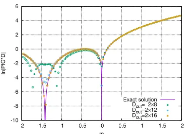
Figures1and 2show the partition function of free Majorana–Wilson fermions, which are computed by the TRG with a fixed bond dimensionDcutand periodic boundary conditions. Specifically, we
compute Eq. (10) with
D=∂/s−2r∂∗µ∂µ+m. (24)
To compute it, we use the Grassmann TRG [14,15], which has been extended to relativistic fermion systems in Refs. [8,10]. We follow Ref. [10] for the coarse-graining procedure except for the defi-nition ofDcut. It is defined as the dimension ofxn =(xn,f,xn,b)in this report, on the other hand, it is
defined as the dimension ofxn,bin Ref. [10], wherexn,f(b)represents the fermionic (bosonic) index of
tensor (see Ref. [10]).
The results for 2×2 and 32×32 space-time lattice are shown in Figs.1and 2, respectively, and for 32×32 case, the relative error is shown. The behavior of numerical errors is qualitatively the same in each case. From the viewpoint of data compression, the largerDcutcontains the more information,
and the results of largerDcutprovides the more accurate results as expected. There are fermion zero
modes atm = 0.0 andm = −√2, and the error grows near such points. The Pfaffian flips its sign
depending on the value ofm, and this reflects the fact that the Pfaffian is not positive definite.
3.2 Witten index of free Wess–Zumino model
Figures3and4show the partition functions of the free Wess–Zumino model whose superpotential is given by
Wfree(ϕ)= 1
2mϕ2. (25)
where
T(xn,1,xn,2,xn,b)(tn,1,tn,2,tn,b)(xn−ˆ1,1,xn−ˆ1,2,xn−ˆ1,b)(tn−ˆ2,1,tn−ˆ2,2,tn−ˆ2,b)
=
K ∑
χ1n,χ2n=1
TF
xn,1xn,2tn,1tn,2xn−ˆ1,1xn−ˆ1,2tn−ˆ2,1tn−ˆ2,2
(
xχ1n )
wχ1nwχ2ne x2
χ1n+x
2
χ2n
·U1 χn,xn,b
√ σ1xn,bU
2 χn,tn,b
√ σ2tn,b
√ σ1xn−ˆ1,bV
1†
xn−ˆ1,b,χn √
σ2tn−ˆ2,bV
2†
tn−ˆ2,b,χn. (23)
Note that the two types of approximation are introduced, the Gauss–Hermite quadrature for the in-tegrals of scalar fields and the truncated singular value decomposition. The tensor indexxn,1(2) and
xn,b run from 0 to 1 and from 1 to DB, respectively. Then, the dimension of the integrated index
xn=(xn,1,xn,2,xn,b)is 2×2×DB, and we call it as the bond dimensionDinit. This notation is followed
in next section.
3 Numerical results
3.1 Partition functions of free Majorana–Wilson fermions
Figures1and 2show the partition function of free Majorana–Wilson fermions, which are computed by the TRG with a fixed bond dimensionDcutand periodic boundary conditions. Specifically, we
compute Eq. (10) with
D=∂/s−2r∂∗µ∂µ+m. (24)
To compute it, we use the Grassmann TRG [14,15], which has been extended to relativistic fermion systems in Refs. [8,10]. We follow Ref. [10] for the coarse-graining procedure except for the defi-nition ofDcut. It is defined as the dimension ofxn =(xn,f,xn,b)in this report, on the other hand, it is
defined as the dimension ofxn,bin Ref. [10], wherexn,f(b)represents the fermionic (bosonic) index of
tensor (see Ref. [10]).
The results for 2×2 and 32×32 space-time lattice are shown in Figs.1and 2, respectively, and for 32×32 case, the relative error is shown. The behavior of numerical errors is qualitatively the same in each case. From the viewpoint of data compression, the largerDcutcontains the more information,
and the results of largerDcutprovides the more accurate results as expected. There are fermion zero
modes atm = 0.0 andm = −√2, and the error grows near such points. The Pfaffian flips its sign
depending on the value ofm, and this reflects the fact that the Pfaffian is not positive definite.
3.2 Witten index of free Wess–Zumino model
Figures3and4show the partition functions of the free Wess–Zumino model whose superpotential is given by
Wfree(ϕ)=1
2mϕ2. (25)
The partition functions are computed with periodic boundary conditions and called the Witten index which is regarded as an indicator of the supersymmetry breaking [16]. The relative error is shown in 8×8 space-time volume case. In this subsection, we fix the degree of the Hermite polynomial for bothϕandHas K =64. The tensor in Eq. (22) hasD4init =(2×2×DB)4components at the initial
-10 -8 -6 -4 -2 0 2 4 6
-2 -1.5 -1 -0.5 0 0.5 1 1.5 2
ln|PfC*D|
m
Exact solution Dcut= 2×8
Dcut=2×12
Dcut=2×16
Figure 1: The partition function of two dimensional free Majorana–Wilson fermions as a function ofmon a 2×2 lattice. The positive and negative sign of the par-tition function are represented as solid and open sym-bols, respectively.
1e-07 1e-06 1e-05 0.0001 0.001 0.01 0.1
-2 -1.5 -1 -0.5 0 0.5 1 1.5 2
δ
m
Dcut= 2×8 Dcut=2×12
Dcut=2×16
Figure 2: The relative error of the partition function of two dimensional free Majorana–Wilson fermions as a function ofmon a 32×32 lattice. The positive and negative sign of the partition function are represented as solid and open symbols, respectively.
stage, and it can grow in coarse-graining steps. We apply the GTRG also in this subsection and cut the growth of the bond dimension byDcut.
In the case of the free Wess–Zumino model, the exact solution of the Witten index is known to be exactly one even on the lattice, and one can see that the larger bond dimension provides the more accurate results. Thus we can conclude that the tensor network representation in Eq. (22) is correct. The reason of low accuracy in the smallmregion is vanishing of the mass term. This means vanishing of the damping factor in the LHS of Eq. (18). If one thinks of the interacting case, theϕ4interaction
term guarantees the fast damping of f, and such a bad property will go away.
0.75 0.8 0.85 0.9 0.95 1
0.2 0.4 0.6 0.8 1 1.2 1.4 1.6 1.8 2 ZP
m
Exact solution Dinit=2×2×16 Dinit=2×2×24 Dinit=2×2×32
Figure 3: The Witten index for the free case as a func-tion ofmon a 2×2 lattice.
0.0001 0.001 0.01 0.1 1
0.2 0.4 0.6 0.8 1 1.2 1.4 1.6 1.8 2
δ
m
Dinit=2×2×16, Dcut=2×32
Dinit=2×2×24, Dcut=2×48 Dinit=2×2×32, Dcut=2×64
4 Summary and outlook
We have constructed a tensor network representation of the two dimensional latticeN = 1 Wess–
Zumino model, and the correctness of the new formulation is confirmed numerically. Now we are ready to turn to the interacting case whose superpotential is given by
Winteraction(ϕ)=1
3gϕ3−
m2
4gϕ, (26)
whereg is the coupling constant. The model is known to exhibit the spontaneous supersymmetry
breaking in the presence of interaction. To check whether the phase structure is consistent with pre-vious results in Ref. [5] or not, we can compute the vacuum expectation value of the scalar field or fermionic/bosonic Green’s functions using the methods described in Ref. [17]. We are now working
in this direction.
Another possible approach to supersymmetric lattice field theories is the domain-wall discretiza-tion for fermions and bosons. The coarse-graining technique for higher dimensional fermion systems is invented in Ref. [18], and the computational cost might be reasonable in three dimensions.
Acknowledgments
We thank Dr. Y. Shimizu for helpful discussions. This work is supported in part by JSPS KAKENHI Grant Numbers JP16K05328, JP17K05411, Grants-in-Aid for Scientific Research from the Ministry of Education, Culture, Sports, Science and Technology (MEXT) (Nos. 15H03651), MEXT as “Ex-ploratory Challenge on Post-K computer (Frontiers of Basic Science: Challenging the Limits)”, and the MEXT-Supported Program for the Strategic Research Foundation at Private Universities Topolog-ical Science (Grant No. S1511006).
References
[1] J. Wess, B. Zumino, Nucl. Phys.B70, 39 (1974) [2] S. Ferrara, Lett. Nuovo Cim.13, 629 (1975)
[3] S. Catterall, S. Karamov, Phys. Rev.D68, 014503 (2003),hep-lat/0305002
[4] C. Wozar, A. Wipf, Annals Phys.327, 774 (2012),1107.3324
[5] K. Steinhauer, U. Wenger, Phys. Rev. Lett.113, 231601 (2014),1410.6665
[6] M. Levin, C.P. Nave, Phys. Rev. Lett.99, 120601 (2007),cond-mat/0611687
[7] Y. Shimizu, Chin. J. Phys.50, 749 (2012)
[8] Y. Shimizu, Y. Kuramashi, Phys. Rev.D90, 014508 (2014),1403.0642
[9] Y. Shimizu, Y. Kuramashi, Phys. Rev.D90, 074503 (2014),1408.0897
[10] S. Takeda, Y. Yoshimura, Prog. Theor. Exp. Phys.2015, 043B01 (2015),1412.7855
[11] H. Kawauchi, S. Takeda, Phys. Rev.D93, 114503 (2016),1603.09455
[12] J. Bartels, G. Kramer, Z. Phys.C20, 159 (1983)
[13] M.F.L. Golterman, D.N. Petcher, Nucl. Phys.B319, 307 (1989) [14] Z.C. Gu, F. Verstraete, X.G. Wen (2010),1004.2563
[15] Z.C. Gu, Phys. Rev.B88, 115139 (2013),1109.4470
[16] E. Witten, Nucl. Phys.B202, 253 (1982)
[17] Z.C. Gu, M. Levin, X.G. Wen, Phys. Rev.B78, 205116 (2008),0806.3509