Scholarship@Western
Scholarship@Western
Electronic Thesis and Dissertation Repository
11-26-2018 1:30 PM
Transient Analysis of Full Scale and Experimental Downburst
Transient Analysis of Full Scale and Experimental Downburst
Flows
Flows
Junayed Chowdhury
The University of Western Ontario
Supervisor Hangan,Horia
The University of Western Ontario
Graduate Program in Civil and Environmental Engineering
A thesis submitted in partial fulfillment of the requirements for the degree in Master of Engineering Science
© Junayed Chowdhury 2018
Follow this and additional works at: https://ir.lib.uwo.ca/etd
Part of the Aerodynamics and Fluid Mechanics Commons, Civil and Environmental Engineering Commons, Environmental Design Commons, and the Mechanical Engineering Commons
Recommended Citation Recommended Citation
Chowdhury, Junayed, "Transient Analysis of Full Scale and Experimental Downburst Flows" (2018). Electronic Thesis and Dissertation Repository. 5861.
https://ir.lib.uwo.ca/etd/5861
This Dissertation/Thesis is brought to you for free and open access by Scholarship@Western. It has been accepted for inclusion in Electronic Thesis and Dissertation Repository by an authorized administrator of
i
Downbursts are highly transient natural phenomena which produce strong downdrafts evolving
from a cumulonimbus cloud They induce an outburst of damaging winds on or near to the
ground causing an immense damage to the ground mounted structures and aircrafts. This study
investigates the transient nature of downbursts using wind speed records from full scale
downburst events employing an objective methodology. This method can detect the abrupt
change points in a downburst time series based on statistical parameters such as mean, standard
deviation and linear trend. In addition to the analysis of the full scale downburst events, several
large scale experimental model downbursts are produced in the Wind Engineering, Energy and
Environment (WindEEE) Dome at Western University by varying downdraft jet diameter and
jet velocity to comprehensively characterize the downburst flow field. High resolution surface
layer data is captured using Cobra probes and dynamics of the downburst vortices is
investigated using Particle Image Velocimetry (PIV) Technique. The analysis of wind speed
record is carried out deploying the moving mean approach with different averaging times.
Statistical analysis on turbulence using reasonable averaging time shows the similarities of
experimental model with full scale events. For the first time, an effort has been made to
compare the primary vortex structure and its evolution with the limited full scale downburst
records obtained using Doppler radar measurements.
Keywords
Downburst, Full scale events, Change points, Transient features, Cobra probe, PIV, Time
ii
Co-Authorship Statement
Chapter Two will be submitted to the Monthly Weather Review journal for publication under
the co-authorship of Romanic D., Junayed C., Jubayer C. and Hangan H.
Romanic D. supervised and organized the manuscript. Junayed C. collected the data, analyzed
and produced all the figures to explain the result. Junayed C. also wrote part of the manuscript.
Romanic D. analyzed the results and wrote most of the part of the manuscript, interpreted
results and conducted literature review. Jubayer C. collected data and helped with writing the
result section as well as reviewing the manuscript. Hangan H. framed and supervised overall
research and commented on the analysis.
Chapter Three will be submitted to the Journal of Wind Engineering and Industrial
Aerodynamics under the co-authorship of Junayed C., Jubayer C., Parvu D., Romanic D., and
Hangan H.
Junayed C. conducted the literature review, analyzed the data. Junayed C. also produced the
figures and results, wrote the overall manuscript. Jubayer C. and Parvu D. performed Cobra
Probe and PIV experiments where Jubayer C. also contributed with the analysis of the cobra
probe data and . reviewed the paper. Romanic D. helped with evaluating the results, reviewed
and commented on the analysis. Hangan H. supervised the research, recommended the
iii
Acknowledgments
I would like to express my sincere gratitude to my research supervisor Dr. Horia Hangan for
his encouraging support and guidance throughout the course of this research work. His
extensive knowledge in wind engineering has encouraged and enlightened me all throughout
the completion of my master’s degree.
I would also like to thank my thesis examiners Dr. Girma Bitsuamlak, Dr. Han-Ping Hong and
Dr. C.T. DeGroot for making some time in between their busy schedule’s to evaluate my thesis
work.
My sincere thanks to Dr. Jubayer Chowdhury, who has supported me unconditionally and
extensively all throughout this thesis. Whenever I had any difficulties with understanding
materials in this field of study, I was sure that I would receive the highest assistance from him.
I would like to extend my thanks to Dr. Djordje Romanic for helping me understanding critical
issues in my thesis particularly with the writing results where his depth of knowledge always
provided the best answers to my questions.
I would again like to thank my co-authors of my on-going publications -Dr. Jubayer
Chowdhury, Dr. Djordje Romanic, Dan Parvu for sharing their knowledge and time that has
made these publications possible.
During this thesis, I was fortunate to have excellent support from my colleagues from my
research group. Sharing the same office space with Mohammed Karami and Julien Lotufo, and
later on with Arash Ashrafi, we had long research related discussions that helped me to grow
my understandings in wind engineering. Especially Mohammed Karami, who helped me with
the study materials and learn software’s related to this research work. In spite of his busy
schedule as a Ph.D. student himself, he was always there to solve any issues that I had with my
research. Aya Kassab, Marilena Enus has helped me sharing their thoughts about my thesis
during my presentations that helped me to find the critical issues to address in my thesis. I
would also like to thank Anant Gairola for reviewing the introduction part of my thesis and
iv
I would like to extend my thanks to Gerald Defoe, Dr. Jubayer Chowdhury, Dan Parvu, for
conducting the experiments in WindEEE and Julien Lotufo for helping me with the setup
procedures for the experiments critically important for this thesis work. I would also like to
thank Adrian Costache for all his technical support during the experiments and overall the
course of my master’s degree.
A special thanks to all the professor whose courses I attended during my Master’s degree (Dr.
Horia Hangan-Wind Engineering, Wind Energy, Dr. Girma Bitsuamlak-Building
Sustainability, Prof. Giovanni Solari-Wind Excited and Aeroelastic Response of Structures,
Dr. Ayman El Ansary- Finite Element and Method).
I would like to acknowledge the financial supports from the Department of Civil and
Environmental Engineering at Western University and Natural Sciences and Engineering
Research Council of Canada (NSERC) Discovery grants.
Lastly and most importantly the support from my family, my parents Jigar Khairun Nafia and
Mir Hossain Chowdhury, My sister-in-law Easmine Akter, My brother Jubayer Chowdhury
for their encouraging support whenever I was feeling unnerved and shared my thoughts without
any hesitation. My three years old niece Zuhaira who has given me strength and peace just
even looking at her. And Tanzuma Islam, who was always there for me. Without their support,
v
Table of Contents
Abstract ... i
Keywords ... i
Co-Authorship Statement... ii
Acknowledgments... iii
Table of Contents ... v
List of Tables ... viii
List of Figures ... ix
List of Appendices ... xiii
Nomenclature ... xiv
Chapter 1 ... 1
1 Introduction ... 1
1.1 General introduction ... 1
1.2 Definition of Downburst ... 1
1.3 Classification of Downburst ... 3
1.4 Literature Review... 5
1.4.1 Downburst field studies ... 5
1.4.2 Numerical and physical simulations ... 11
1.5 Motivation and purpose of this thesis ... 17
1.6 Organization of this thesis ... 19
1.7 References ... 19
Chapter 2 ... 25
2 Investigation of transient nature of downbursts from Europe, United States and Australia through detection of abrupt changes in wind speed records... 25
2.1 Introduction ... 25
vi
2.2.1 Data ... 31
2.2.2 Change points in downburst wind records-theoretical background ... 32
2.3 Results ... 36
2.3.1 Europe ... 37
2.3.2 The US ... 40
2.3.3 Australia ... 43
2.4 Discussion ... 45
2.4.1 Model sensitivity ... 45
2.4.2 Transient characteristics of downburst time series ... 48
2.4.3 Outlook ... 53
2.5 Conclusions ... 54
2.6 Acknowledgements ... 56
2.7 References ... 60
Chapter 3 ... 66
3 Parametric characterization of large scale experimentally produced downburst flows 66 3.1 Introduction ... 66
3.2 Experimental setup and test cases ... 70
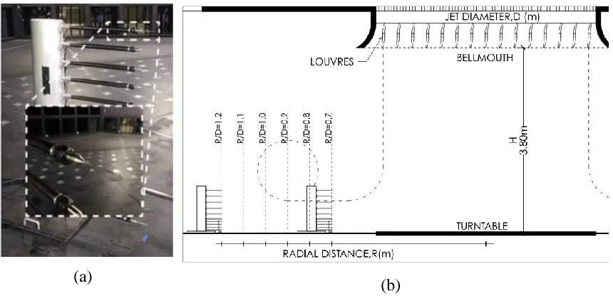
3.2.1 Test chamber (WindEEE Dome) ... 70
3.2.2 Cobra probe setup ... 71
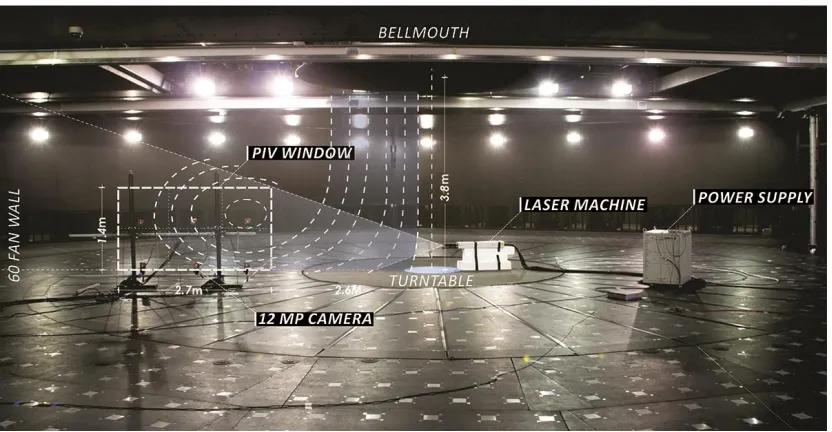
3.2.3 PIV setup ... 73
3.3 Results ... 74
3.3.1 Downburst records analysis and the proper value of moving average period (𝑇𝑎𝑣𝑔) ... 74
3.3.2 Downburst velocity profiles ... 84
3.3.3 Statistical Analysis of Turbulence ... 87
vii
3.4 Summary and Conclusions ... 102
3.5 References ... 104
Chapter 4 ... 112
4 Conclusions and Recommendations ... 112
4.1 Summary ... 112
4.2 Conclusions ... 113
4.3 Recommendation and future work ... 115
4.4 References ... 116
Appendices ... 118
References ... 122
viii
List of Tables
Table 2.1: Downburst events investigated in this paper. See Fig. 2 for their location on map
... 57
Table 3.1: 𝑅𝑒 for different jet diameters and fan speeds ... 72
Table 3.2: The maximum instantaneous radial velocity (𝑢𝑚𝑎𝑥,𝑖) and its location for each of the
investigated cases ... 75
Table 3.3: Average values of 𝜇𝑢̃′, 𝜎𝑢̃′, 𝛾𝑢̃′, 𝜅𝑢̃′ from all six cases ... 83
Table 3.4: The maximum value of the time varying mean radial velocity, 𝑢𝑚𝑎𝑥 and its location
... 84
Table 3.5: The values of 𝑅, 𝐺𝑚𝑎𝑥, 𝐺𝑝𝑒𝑎𝑘 using 𝑇𝑎𝑣𝑔= 0.1 s for all 𝑅𝑒 cases in this study ... 93
ix
List of Figures
Figure 1.1: Differences in flow structure between downburst (microburst) and tornado (NOAA
photo library) ... 2
Figure 1.2: Illustration of four stages of a Downburst event. Descending of air, air hitting the
ground, maturing and spreading out of air radially as runaway vortex rolls (Wolfson, 1988) . 3
Figure 1.3: Schematic of a wet and dry microburst (Fujita, 1990). ... 4
Figure 1.4: Aerial photographs showing the damages by downbursts wind. Trees are blown
(left) in a starburst pattern and an outbuilding (right) was damaged by microburst winds (Fujita,
1990). ... 6
Figure 1.5: Single-Doppler wind data in vertical cross section showing contours of Vertical
windspeed (left) Horizontal wind speed (right) of a microburst during the project NIMROD
(Fujita, 1992, Wilson and Wakimoto, 2001) ... 7
Figure 1.6: Photograph of a Microburst outflow observed in Denver, Colorado during JAWS
project. Dust ring observed on 15 July, 1982 (left) and Outflow of the microburst from heavy
rain shaft on 6 July, 1984 (Right) (Hjelmfelt, 1988). ... 8
Figure 1.7: Time evolution of a microburst seen during the JAWS project. (Wilson et al., 1984,
Hjelmfelt, 1988). ... 9
Figure 1.8: Simulated microburst vorticity field obtained through the PIV experiment
(Alahyari & Longmire, 1994) ... 13
Figure 1.9: Velocity profile for a full scale event from JAWS experiment (Hjelmfelt, 1988)15
Figure 1.10: Comparison of downburst mean velocity profiles between empirical model,
laboratory experiment and typical boundary layer profiles (Kim and Hangan, 2007). ... 16
Figure 2.1: An hour-long time series of (a) steady atmospheric boundary layer (ABL) wind
x
Figure 2.2: Location map of downburst events in (a) Europe, (b) United States and (c) Australia
... 31
Figure 2.3: All downburst records investigated in this study ... 36
Figure 2.4: Three segmentation methods applied to a downburst records from Genoa (left
panels) and a downburst record from Livorno (right panels). ... 38
Figure 2.5: Same as Figure 2.4 but for one La Spezia event (left panels) and one Livorno event
(right panels). Notice that the downburst signatures in this figure and Figure 2.4 are noticeably
different; see text for further discussion. ... 40
Figure 2.6: Three segmentation methods applied to a downburst records from Syracuse (left
panels) and Pep (right panels). ... 42
Figure 2.7: Three segmentation methods applied to a downburst records from Lubbock (left
panels) and Washington (right panels). ... 43
Figure 2.8: Three segmentation methods applied to a downburst records from Australia. .... 44
Figure 2.9: The number of detected change points versus 𝛾 for three different sampling
frequencies. ... 46
Figure 2.10: Dependency of 𝛾 on sampling frequency, 𝑓𝑠, for the mean cost function. ... 47
Figure 2.11: (a) Downburst durations determined using M, SD and LT approaches for time
records listed in Table 1. (b, c, d) Histograms of downburst durations obtained by M, SD and
LT approaches, respectively. ... 49
Figure 2.12: Same as Figure 2.10, but for downburst ramp-up time. ... 50
Figure 2.13: (a) The ratio (R𝑑𝑝/𝑏𝑝) of mean wind speeds during downburst peak (dp) and before
peak (bp), as well as the ratio (R𝑑𝑝/𝑎𝑝) of the mean wind speeds during dp and after peak (ap).
(b, c) Histograms of R𝑑𝑝/𝑏𝑝 and R𝑑𝑝/𝑎𝑝, respectively. ... 52
xi
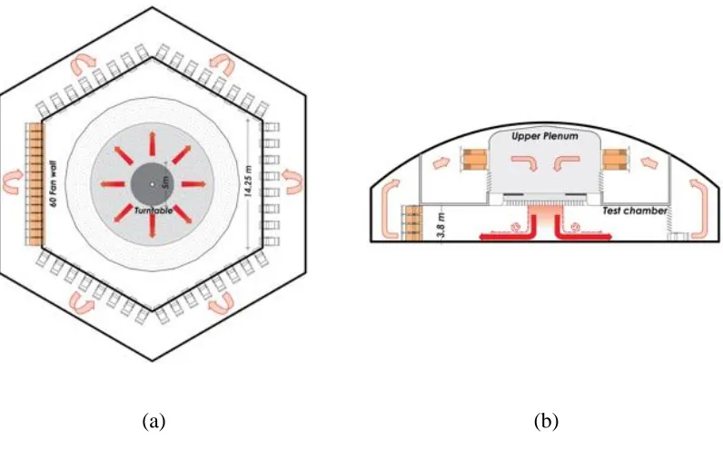
Figure 3.1: Schematic of (a) horizontal and (b) vertical sections of the WindEEE Dome
downburst mode. ... 71
Figure 3.2: (a) Mast equipped with 12 Cobra probes (b) Schematics of the location of the
measuring mast and Cobra probes in the WindEEE Dome testing chamber ... 72
Figure 3.3: PIV setup ... 73
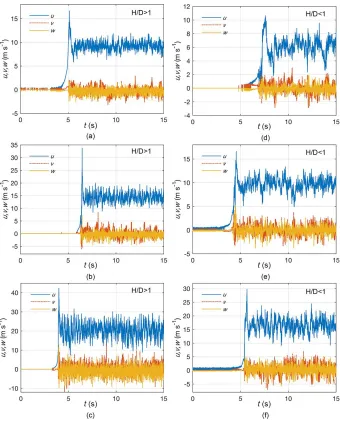
Figure 3.4: Radial (𝑢), lateral (𝑣) and vertical (𝑤) components of instantaneous velocity for
𝑅𝑒 (a) 1.83 × 10⁶, (b) 2.62 × 10⁶, (c) 4.24 × 10⁶, (d) 1.82 × 10⁶, (e) 2.68 × 10⁶ and (f) 4.09 ×
106 ... 75
Figure 3.5: Abrupt changes in the signal (dashed lines) used to determine the initial point of
the gust front (first dashed line) for (a) Re=1.83 × 10⁶ and (b) 𝑅𝑒=1.82 × 10⁶ ... 77
Figure 3.6: Time history of the 𝑢 velocity component and its decomposition for the case of
𝑅𝑒 = 1.83 × 10⁶ and 𝐻𝐷 > 1 obtained by using different values of 𝑇𝑎𝑣𝑔: (a) 0.01 s, (b) 0.025
s, (c) 0.05 s, (d) 0.1 s, (e) 0.2 s, and (f) 0.3 s. ... 80
Figure 3.7: Derived functions based on the Fourier transform of 𝑢(𝑡) and 𝑢′(𝑡), 𝑛|𝐹𝑢̅|2,
𝑛|𝐹𝑢′|2 and 𝑛|𝐹𝑢̅||𝐹𝑢′|, for 𝑅𝑒 =1.83 × 10⁶ and 𝐻/𝐷>1. The panels indicate different values
of 𝑇𝑎𝑣𝑔 that were used to obtain 𝑢(𝑡) and 𝑢′(𝑡): (a) 0.01 s, (b) 0.025 s, (c) 0.05 s, (d) 0.1 s, (e)
0.2s and (f) 0.3 s ... 82
Figure 3.8: Downburst radial velocity profiles at the radial location of 𝑢𝑚𝑎𝑥 (a) without
normalization and (b) normalized ... 85
Figure 3.9: Normalized velocity profiles from full scale events are plotted against the
experimentally generated downbursts in the WindEEE Dome ... 86
Figure 3.10: Vertical profiles of 𝑢(t) at different time instances in the time series and at the
radial location of 𝑢𝑚𝑎𝑥 . The investigated case is for 𝑅𝑒=2.62 × 10⁶ and 𝐻/𝐷 >1. (a) Moving
mean time series and (b) vertical profiles at different time instances, 𝑡=0.34 to 0.58 s (i)–(vii)
xii
Figure 3.11: PSD of the reduced turbulence fluctuations matched with n − 53 profile (red line)
using 𝑇𝑎𝑣𝑔 = 0.1 s for 𝑅𝑒, (a) 1.82 × 10⁶, (b) 2.62 × 10⁶, (c) 4.09 × 10⁶, (d) 1.83 × 10⁶, (e) 2.68
× 106 and (f) 4.24 × 10⁶ ... 89
Figure 3.12: PSD of the reduced turbulence fluctuations (𝑇𝑎𝑣𝑔 = 0.1 s) matched against the
analytical model proposed by Solari and Piccardo (2001) (red line) for 𝑅𝑒 (a) 1.83 × 10⁶, (b)
2.62 × 10⁶, (c) 4.24 × 10⁶, (d) 1.82 × 10⁶, (e) 2.68 × 10⁶ and (f) 4.09 × 10⁶ ... 90
Figure 3.13: PDF of the reduced turbulent fluctuations (𝑇𝑎𝑣𝑔 = 0.1 s) for 𝑅𝑒 (a) 1.83 × 10⁶,
(b) 2.62 × 10⁶, (c) 4.24 × 10⁶, (d) 1.82 × 10⁶, (e) 2.68 × 10⁶ and (f) 4.09 × 10⁶. Red line represents a Gaussian PDF... 92
Figure 3.14: PIV vectors and velocity magnitude contours for 𝐻/𝐷<1 and 𝑅𝑒= 2.68×10⁶ at
different time instances. Time interval between two consecutive instances is 0.11s. ... 95
Figure 3.15: (a) Vector plot with velocity magnitude from PIV experiment with the location of
the maximum velocity and the centre of the vortex for 𝐻/𝐷<1 and 𝑅𝑒= 2.68 × 10⁶, (b) velocity
magnitude plotted against normalized radial distance and (c) schematic of the downburst flow
field and the location of the maximum velocity obtained using the full scale data from the
JAWS campaign (Hjelmfelt, 1988) ... 97
Figure 3.16: Streamline plots showing the primary vortex at different instances for H/D<1 and
𝑅𝑒= 2.68 ×10⁶ ... 98
Figure 3.17: Streamlines showing the second vortex after passing of the primary vortex for
𝐻/𝐷<1 and 𝑅𝑒= 2.68 ×10⁶ ... 99
Figure 3.18: Trajectory of the vortex centre for different values of 𝑅𝑒. ... 100
Figure 3.19: Comparison of vortex centre heights from the WindEEE Dome downbursts and
full scale events on (a) 16 June 1978 (b) 17 June 1978 (Wakimoto, 1982) ... 101
Figure 3.20: Normalized vortex trajectories from the WindEEE Dome downbursts compared
xiii
List of Appendices
Appendix A: Figures presented here are in support of the Chapter 3. ... 118
xiv
Nomenclature
Abbreviations
ABL Atmospheric Boundary Layer
AGL Above Ground Level
CS Cloud Simulation
CLAWS Classify, Locate and Avoid Wind Shear
CP-3 Coherent Pulsed 3
CMOS Complementary Metal-Oxide Semiconductor
EF-3 Enhanced Fujita 3
ESDU Engineering Science Data Unit Standard
GRF Gust Response Factor
JAWS Joint Airport Weather Studies
LT Linear Trend
MIST Microburst and Severe Thunderstorm Project
M Mean
NCAR National Center for Atmospheric Research
NIMROD National Intensive Meteorological Research on Downbursts
PDF Probability Density Function
PIV Particle Image Velocimetry
PSD Power Spectral Density
RMS Root Mean Square
xv
SD Standard Deviation
TFI Turbulent Flow Instrumentation
WindEEE Wind Engineering Energy and Environment
Symbols
𝐷 Downburst jet diameter m
FS Fan speed %
𝑓𝑠 Sampling frequency Hz
𝐹𝑢̅ Fourier transform of time varying mean -
𝐹𝑢′ Fourier transform of residual fluctuation -
𝐺 Gust factor -
𝐺𝑚𝑎𝑥 Ratio between maximum instantaneous velocity
with maximum moving mean velocity
-
𝐺̂ Ratio between 1-s peak velocity with maximum
moving mean velocity
-
𝑔 Gust response factor -
𝐻 Height of the Downburst m
𝐼𝑢 Turbulence Intensity -
𝐿𝑣 Maximum of the moving mean velocity m/s
𝑛 Sampling frequency Hz
𝑅 Radial distance m
𝑅̂ Ratio between maximum instantaneous velocity
with 1-s peak velocity
-
xvi
𝑅𝑐𝑚 Radial distance of the vortex core at minimum
height
m
𝑅𝑑𝑝 𝑏𝑝⁄ Ratio between the mean wind speed during
downburst peak and before downburst peak
-
𝑅𝑑𝑝 𝑎𝑝⁄
Ratio between the mean wind speed during
downburst peak and after downburst peak
-
𝑆𝑢̃′ Power spectral density of 𝑢̃′ -
𝑇𝑎𝑣𝑔 Averaging time s
𝑇𝑖𝑖 Insertion instance of the vortex into the region s
𝑇𝑒𝑖 Ending instance of the vortex passing the region s
𝑇𝑖𝑛𝑡 Time interval of the instances s
𝑡𝑠 Sampling time s
𝑡 Time s
𝑈̂1m 1-min maximum wind speed m/s
𝑈̅− Pre peak mean wind speed m/s
𝑈̅+ Post peak mean wind speed m/s
𝑢 Instantaneous radial wind velocity m/s
𝑢̅ Time varying mean of radial velocity component m/s
𝑢′ Residual fluctuation of radial velocity component m/s
𝑢̃′ Reduced turbulent fluctuation of 𝑢 -
𝑢̂ 1-s peak radial wind speed m/s
𝑢𝑚𝑎𝑥 Maximum instantaneous radial velocity m/s
𝑢̅𝑚𝑎𝑥 Maximum running mean radial velocity m/s
𝑢𝑚𝑎𝑥,𝑖 Instantaneous maximum radial velocity m/s
xvii
𝑈̅𝑏𝑝 Mean wind speed before downburst peak m/s
𝑈̅𝑎𝑝 Mean wind speed after downburst peak m/s
𝑢𝑐𝑜 Primary vortex core convective velocity m/s
𝑣 Instantaneous lateral wind velocity m/s
𝑣 Instantaneous wind speed m/s
𝑣̅ Time varying mean wind speed m/s
𝑣′ Residual fluctuation m/s
𝑣̃′ Reduced turbulent fluctuation -
𝑣̂ Peak response m/s
𝑣̅𝑇𝑉𝑀 Largest response to time varying mean m/s
𝑤 Instantaneous axial (vertical) wind velocity m/s
𝑍 Height of the cobra probe m
𝑍𝑐𝑚 Minimum height of the vortex core in vortex
trajectory
m
𝑍𝑚𝑎𝑥 Height of the maximum moving mean velocity m
𝑍𝑚𝑎𝑥,𝑖 Height of the maximum instantaneous velocity m
Greek Symbols
𝜎𝑣 Slowly varying standard deviation m/s
𝜎𝑢 Standard deviation of radial velocity component m/s
𝜎𝑢̃′ Standard deviation of 𝑢̃′ -
𝜎𝑑𝑝 Standard deviation during downburst peak m/s
xviii
𝜎𝑎𝑝 Standard deviation after downburst peak m/s
𝜎𝑑𝑝 𝑏𝑝⁄ Ratio between the standard deviation during
downburst peak and before downburst peak
-
𝜎𝑑𝑝 𝑎𝑝⁄ Ratio between the standard deviation during
downburst peak and after downburst peak
-
𝜇𝑢̃′ Mean value of 𝑢̃′ -
𝛾𝑢̃′ Skewness value of 𝑢̃′ -
𝜅𝑢̃′ Kurtosis value of 𝑢̃ -
𝜃𝑒 Maximum vertical differential -
𝜏 Short time interval s
Chapter 1
1
Introduction
1.1
General introduction
On June 1975, an aircraft from Eastern Airlines affronted with a rapid diverging wind while
attempting to land at New York’s John F. Kennedy Airport (JFK) crashed and killed 112
people. This divergent wind pattern was recorded previously while the starburst pattern of
fallen trees was visible in an aerial survey from the damages of ‘super-outbreak’ of 148
tornadoes on 3-4 April 1974 (Fujita, 1974). Similarities in the wind pattern of these two
events were found based on the investigation of the recorded data from the aircraft flight
data recorder. From all this analysis Fujita termed the event as ‘Downburst’ and defined it
as ‘A natural event that occurs due to thunderstorms produced by a cumulonimbus cloud
causing a strong downdraft which induces an outburst of damaging winds on or near the
ground’ (Fujita, 1990). This radially divergent wind with high wind velocity transpires
when descending air hits the ground causing immense damage to the ground-mounted
structures.
Downburst is defined in the next section followed by the classifications of downbursts.
Previous studies on downbursts and their findings as well as limitations are described in
the literature review section. This chapter ends with the motivation and organization of the
thesis as well as a list of the cited references.
1.2
Definition of Downburst
Downbursts were primarily defined exclusively for aviation purposes during 1976 and
1977. Later, it was redefined meteorologically as scientists reveal the scale and nature of
this phenomenon (Fujita and Wakimoto, 1981). In nature, downbursts can be identified as
rotating air towards the ground. While reaching the ground, this sudden downfall bursts
out violently causing an immediate rise in the wind velocity in the lower region of the
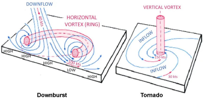
ground (Fujita, 1990). Figure 1.1 shows the fundamental differences in flow structure
between downburst and tornado.
Figure 1.1: Differences in flow structure between downburst (microburst) and
tornado (Adapted from NOAA photo library)
According to Byers and Braham (1948) a thunderstorm evolves in three stages. During the
first stage, air rises vertically. At the second stage, both the rising and sinking air co-exists
and in the final stage the cloud breaks up and strong sinking current hits the ground
producing downbursts. This rising and sinking currents are termed as ‘Updraft’ and
‘Downdraft’ respectively. Formation of a downburst is a density-driven incident in the
atmosphere. This density driven incident is caused by thermodynamic cooling associated
with the formation of the thunderstorm cloud itself. Inside the thunderstorm cloud, the
thermodynamic process causes air density to rise in the volume of clouds which eventually
results into a massive downdraft with precipitation in the form of rain, snow, hail and
graupel (Wakimoto, 1985). The precipitation sometimes aids in the downdraft to gain
greater strength and accelerate the thunderstorm air parcels downward (Wolfson, 1988).
midair microburst descends, Contact stage: microburst hits the ground, Mature stage:
stretching of the ring vortex, Breakup stage: runaway vortex rolls induce burst swaths) and
these stages are illustrated in Figure 1.2.
Figure 1.2: Illustration of four stages of a Downburst event. Descending of air, air
hitting the ground, maturing and spreading out of air radially as runaway vortex
rolls (Adapted from Wolfson, 1988)
1.3
Classification of Downburst
Primarily Fujita (1990) classified downburst into Microburst and Macroburst. A
macroburst is a large-scale downburst which has a damaging wind extending over 4 km (>
2.5 miles) and a microburst is a small downburst which has a damaging wind extending up
to 4 km (≤ 2.5 miles) horizontally. Based on the observations and analyses, Fujita (1990)
postulated that a microburst can produce wind gusts as high as 75 m/s, whereas a
microburst can last for about 2-5 minutes, on the other hand, a macroburst can last up to
30 minutes.
Due to its short span in time and high intensity, the maximum wind speed of microbursts
is expected to be higher than that of macroburst (Fujita, 1974). The intensity of a downburst
is usually much less than that of a tornado, but sometimes their intensity may reach as high
as F3. Of the 142 downbursts that Fujita observed during his survey in between 1976 and
1978, 98.6% were F2 or weaker, none were F4 or stronger, but 1.4% were as strong as F3
(Fujita, 1978).
Additional classification of downburst emerged while several full scale projects were
conducted to understand its character. While pursuing the projects NIMROD (Northern
Illinois Meteorological Research on Downbursts) (Fujita, 1978), JAWS (Joint Airport
Wind Shear) (Wilson et al., 1984; Hjelmfelt, 1988) and MIST (Microburst and Severe
Thunderstorm) (Fujita, 1990), three types of downburst were detected and observed.
During JAWS, strong microburst winds were recorded without sufficient rainfall on the
ground and was classified as dry microburst (Fujita, 1990). Cloud base in the MIST project
near Huntsville, AL was at a very low elevation and the downburst was accompanied by
heavy rain. Fujita classified this event as a wet microburst. A schematic of this
classification is shown in Figure 1.3.
According to the damage patterns, downbursts were again classified into five scales (Fujita
and Wakimoto, 1981). Downburst swaths can have lengths from tens of meters to several
hundred kilometers. From the downbursts that occurred on 16 July 1980, five different
meteorological scales were classified. Based on the damage pattern these scales were
classified as a family of Downbursts clusters (Maso-BETA scale), Downburst cluster
(Meso-ALPHA scale), Downburst (Meso-BETA scale), Microburst (Miso-ALPHA scale)
and Burst swath (miso-BETA scale). These five categories are branched under the two
significant sub-categories which are ‘Masoscale’ and ‘Misoscale’. Each of this scales are
also divided into ALPHA (larger) and BETA (smaller) scales for subscale identification
(Fujita and Wakimoto, 1981).
1.4
Literature Review
In this section previous studies on downbursts and their flow characteristics are discussed.
These studies can be divided into three main categories, field measurements of full scale
downbursts, experiments with model scale downbursts and numerical simulations. In
Section 1.4.1, projects capturing full scale downburst events and their major findings are
discussed. Section 1.4.2 presents different experimental and numerical techniques to
simulate downbursts and how these techniques vary from one another. The importance and
effects of downbursts related to wind engineering are also explained here.
1.4.1 Downburst field studies
Fujita first identified downbursts back in 1976 from a set of aerial photographs.
Investigating the damages in the wake of the super out-break of tornadoes on 3-4 April
1974, Fujita found a strange pattern which changed his vision towards the damages by the
storm. He found that the trees were blown out in a starburst pattern, which is similar to the
damage caused by a jet of descending air as it hits the ground and burst out violently. From
is a strong downdraft inducing an outburst of damaging winds on or near the ground (Fujita,
1978).
A series of field studies were conducted during the 1970s and 1980s to know more about
the characteristics of downbursts. The first field study was the project NIMROD during the
spring and summer of 1978. The primary objective of NIMROD was to study and validate
the existence of downbursts and to collect meteorological data on a nationwide scale. After
the crash of an Airliner short of the runway of John F. Kennedy Airport, New York on June
24, 1975, the National Transportation Safety Board called for an investigation to prevent
further sinking of airplanes due to the sharp wind changes under thunder showers.
(a) (b)
Figure 1.4: Aerial photographs showing the damages by downbursts wind. (a) Trees
are blown in a starburst pattern and (b) an outbuilding was damaged by microburst
winds (Adapted from Fujita, 1990).
The Project NIMROD starts with the operation of a Triple-Doppler Network in Northern
Illinois in May and June of 1978. Three Doppler radars were placed in the site in close
proximity in order to determine the three- dimensional structure of the downburst airflow.
But to prove the existence of downbursts and increase the likelihood of capturing more
events, Fujita (1978) decided to increase the distance between two radars which set the
wind speed of 31 m/s above 45 m from ground in the western suburbs of Chicago (Wilson
et al., 1984; Fujita, 1990). Approximately 50 downbursts were detected during the project
NIMROD proving their existence and high frequency of occurrence in nature (Wilson and
Wakimoto, 2001). Figure 1.5 shows the horizontal and vertical cross sections of one of the
downburst events captured during NIMROD.
Right after the project NIMROD, researchers like Fujita, Serafin, Wilson and John
McCarthy decided to conduct more experiments to have a better understanding of the
structure, evolution and cause of microbursts over the high plains. As a result Project
JAWS was conducted for 86 days from 15 May to 13 August, 1982 in Colorado, Denver.
The same Doppler radars from NIMROD were used but this time the radars were laid to
capture the three dimensional wind field of the life cycle of a microburst. The spacing
between the two radar was 15, 18 and 28 km, which was much tighter then NIMROD
project (Wilson and Wakimoto, 2001). A total of 186 downbursts were captured during
this time.
(a) (b)
Figure 1.5: Single-Doppler wind data in vertical cross section showing contours of (a)
Vertical wind speed and (b) Horizontal wind speed of a microburst during the project NIMROD (Adapted from Fujita, 1992, Wilson and Wakimoto, 2001)
One of the major findings of JAWS project was that strong downdrafts were not only
beginning, but could also occur in the absence of any significant rain activity at all. Proctor
(1988) analyzed the environmental conditions of June 30, 1982 downburst event and
described how microburst downdraft was initiated by the distribution of precipitation at the
top of the boundary layer. Srivastava (1985, 1987), based on his analytical model,
explained that the equality in sub cloud environmental lapse rate and dry-adiabatic rate, or
even relatively light rainfall can be a reason to produce intense downdrafts which
eventually produce no rain near the ground. This type of event is termed as a dry
microburst. Out of 186 microburst events during the JAWS experiment, 151 were
identified as dry microbursts and the rest were wet microbursts. Figure 1.6 shows the
microburst outflow observed in Denver, Colorado on 15 July 1982. The effect of snow and
hail at the top of the boundary layer to create downdraft is explained later by Proctor
(1988).
(a) (b)
Figure 1.6: Photograph of a Microburst outflow observed in Denver, Colorado
during JAWS project. (a) Dust ring observed on 15 July, 1982 and (b) Outflow of
the microburst from heavy rain shaft on 6 July, 1984 (Adapted from Hjelmfelt,
1988).
Downbursts are accompanied by the formation of an annular vortex developing as a result
of the shear between the descending flow and the still surrounding air mass. The spreading
of microburst after reaching the ground surface was seen by Fujita (1985) in his laboratory
model. In full scale, this radial expansion of outflow happens near the ground (<1 km) with
1988; Fujita, 1990; Mason et al., 2005). Wilson et al. (1984), from the analysis of doppler
radar data from the JAWS project, postulated that the maximum differential wind speed
occurs at a height of approximately 75 m from the ground. This surface layer is of critical
importance for wind engineering. However, the full scale data in the near surface region is
very limited and has very low spatial and temporal resolution. In Figure 1.7 the
development and dissipation of microburst are shown in time.
Figure 1.7: Time evolution of a microburst seen during the JAWS project (Adapted
from Wilson et al., 1984, Hjelmfelt, 1988).
Most of the full scale downburst data found in the literature are either from the United
States (Wakimoto, 1982; Wilson et al., 1984; Hjelmfelt, 1988; Holmes et al., 2008; Gunter
and Schroeder, 2015) or from Europe (Järvi et al., 2007; Solari et al., 2015; Burlando et
al., 2017). There are few downburst datasets available from Asia (Choi and Hidayat, 2002)
and Australia (Sherman, 1987). In comparison to synoptic boundary layer winds,
thunderstorm downburst winds are highly transient in nature. To detect this transient
nature, different methodologies have been proposed (Gomes and Vickery, 1978; Cook et
al., 2003). Gomes and Vickery (1978) proposed the method of applying the extreme-value
analysis method to separate the extreme wind events. Choi and Hidayat (2002) used the
gust factor analysis to separate thunderstorm from non-thunderstorm winds for wind
engineering applications. In Chapter 2 of the thesis, an analysis on separating downburst
winds from synoptic boundary layer winds is discussed in detail.
As a downburst is a non-stationary process, the typical way of using a fixed averaging time
to analyze stationary synoptic wind events, is not appropriate for downburst time series.
Chen and Letchford (2004), Holmes et al. (2008), McCullough et al. (2014), Lombardo et
al. (2014) and Solari et al. (2015). Hong (2016) proposed a model to represent
nonstationary winds using the decomposition of instantaneous power spectrum. Choi and
Hidayat (2002) proposed a running mean approach for thunderstorm winds which provides
more accurate results for the prediction of peak response factor of a structure. In this
process Choi and Hidayat (2002) decomposed the instantaneous wind velocity (𝑣) into a
time varying mean part (𝑣̅) and residual fluctuation (𝑣′) using different averaging time (𝑡).
This can be expressed as Eq. (1.1).
𝑣(𝑡) = 𝑣̅(𝑡) + 𝑣′(𝑡) (1.1)
Based on this method and calculating the spectra of the 𝑣′ for a averaging time ranging
from 10 s to 120 s Choi and Hidayat (2002) postulated an averaging time of 60 s for
downburst events recorded in Tuas, Singapore. Using the similar approach from the dataset
of Lubbock Reese downdraft, Holmes et al. (2008) suggested 40 seconds as the averaging
time for thunderstorm downbursts. Holmes used the criteria of retaining the main features
of downburst time history and near zero mean value for residual fluctuation (𝑣′) as criteria
to determine the averaging time. Lombardo et al. (2014) followed the 2nd criteria suggested by Holmes et al. (2008), which states that 𝑣′ should have a near zero mean value, to obtain
the averaging time. Twenty different averaging time ranging from 1.1 s to 723 s were
applied on downburst events recorded at Reese Technology Center in Lubbock, Texas,
USA. Using additional criteria and based on the analysis on 96 downburst events on ports
of Italy, Solari et al. (2015) used 30 seconds as the averaging time to analyze downburst
events. To find the averaging time Solari et al. (2015) also decomposed the wind velocity
into a slowly varying mean and residual fluctuation which is dealt as a non-stationary
random process. In addition to decomposing the instantaneous wind speeds (𝑣) into 𝑣̅ and
𝑣′, Solari et al. (2015) introduced the analysis of reduced turbulent fluctuation (𝑣̃′) via Eq.
(1.2) which is dealt as a rapidly varying random Gaussian process with a near zero mean
value and unit standard deviation and expressed by Standard deviation of residual
fluctuation (𝜎𝑣).
Solari et al. (2015) also defined three wind speed ratios of importance to loading and
response of structures to downburst winds, i.e:
𝑅̂ = 𝑣𝑚𝑎𝑥 𝑣̂
(1.3)
𝐺𝑚𝑎𝑥 =𝑣𝑚𝑎𝑥 𝑣̅𝑚𝑎𝑥
(1.4)
𝐺̂ = 𝑣̂ 𝑣̅𝑚𝑎𝑥
(1.5)
Here, 𝑣𝑚𝑎𝑥 is the instantaneous maximum of the downburst wind speed, 𝑣̂ is the 1-s peak
wind speed and 𝑣̅𝑚𝑎𝑥 is the maximum of the running mean which is a function of averaging
time, 𝑡.
Field measurements are the most relevant way to study downburst characteristics.
However, it is important to note that capturing full scale downburst events is a challenging
process as duration of downbursts are very short in nature and also difficult to forecast.
Accurate flow visualization near the ground region is sometimes difficult to obtain by
doppler radar technology (Alahyari and Longmire, 1994). Also, as mentioned previously,
data within the surface layer, which is the most critical region for wind engineering
applications, is very limited with low spatial and temporal resolutions. Considering these
difficulties, numerical models (Kim and Hangan, 2007; Mason et al. 2009; Vermeire et al.,
2011; Zhang et al., 2013; Orf et al., 2014) and scaled experimental models (Fujita, 1985;
Alahyari and Longmire, 1994; Mason et al., 2005; Xu and Hangan, 2008; Sengupta and
Sarkar, 2008; Jesson et al., 2013, Zhang et al., 2013) have been developed to study
downbursts. A brief summary of these numerical and experimental studies along with their
significant findings are presented in the following section.
1.4.2 Numerical and physical simulations
For wind engineering purposes, downbursts can be modelled physically and numerically.
three categories: ring-vortex, cooling source and impinging jet modeling. Ring vortex
model is used primarily to understand the main features of the flow field around the primary
vortex in a downburst (Ivan, 1986; Schultz, 1990; Jesson and Sterling, 2018) In the
ring-vortex model, the descending air is modeled as annular ring-vortex ring prior to touching the
ground (Chen and Letchford, 2004). Although the ring vortex model qualitatively captures
the features of primary downburst vortex, impinging jet models have shown to be better in
predicting the radial outflow of downbursts (Holmes and Oliver, 2000; Savory et al., 2001).
In the cooling source (CS) model, negative buoyancy is used for the dynamic development
of the simulated downburst (Vermeire et al., 2011; Orf et al., 2014). Physically this is done
by releasing heavier fluids into lighter fluids which is termed as liquid drop release method
(Lundgren et al., 1992; Alahyari and Longmire, 1994; Yao and Lundgren, 1996). Yao and
Lundgren (1996) modelled an isolated dynamic downburst by releasing salt water solution
from higher elevation into fresh water. This experimental model identified the divergent
flow with vortex ring dissipating form a central impact point. Similar results on the vortex
formation is seen from the experimental model by Fujita (1985). Here it is important to
note that, the experimental model, Yao and Lundgren (1996) showed the presence of a
counter rotating vortex (secondary vortex) at the leading edge of the vortex and very close
to the surface. The reason of development of this counter rotating vortex is the friction
between the shear layer of wind and steady ground surface. In recent experiments Mason
et al. (2005) presented the similar concept of counter rotating vortex. From the experiment
by Lundgren et al. (1992) Yao and Lundgren (1996) Reynolds number dependency in the
model microburst was found only at low Reynolds number and it was noticed that
large-scale turbulent (i.e. primary vortex, secondary vortex) motions are not dominated by
Reynolds number effects.
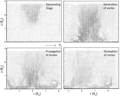
First successful application of particle image velocimetry (PIV) in a variable density flow
was demonstrated by Alahyari and Longmire (1994). One of the major reasons to turn to
PIV experiments was to capture the microburst wind flow field with higher spatial
resolution and less intrusively compared to conventional hot wire anemometry in use at
that time. From the experimental model Lundgren et al. (1992) considered microburst
Maximum velocity was found at 𝑅/𝐷 = 1 where R is the radial distance and D is the jet
diameter (Alahyari and Longmire, 1994). Figure 1.8 shows the descending phase and
generation of vortex from the PIV experiment.
Figure 1.8: Simulated microburst vorticity field obtained through the PIV
experiment (Adapted from Alahyari & Longmire, 1994)
Numerically, negatively-buoyant CS model has been used by Mason et al. (2009),
Vermeire et al. (2011), Zhang et al. (2013) and Orf et al. (2014). Numerical CS models use
thermodynamic cooling from a pre-defined cooling source forcing function that produces
a similar type of downdrafts observed in nature. While these models come closer to
reproducing the physics of real downbursts, they usually run heavy simulations on large
domains and do not emphasize on the details of the surface layer which is of crucial
Impinging jets models have been widely adopted by researchers to investigate microburst
outflow as its relatively simple and has the ability to produce the proper vortex flow
structure and to provide reasonable resolution in the surface layer (Xu and Hangan, 2008;
Zhang et al., 2013). Though the evolution of downbursts in nature is a very complex
process, in laboratory, physical and numerical downbursts are modelled by axi-symmetric,
continuous or impulsively driven circular impinging jets (Letchford and Chay, 2002; Kim
and Hangan, 2007; Xu and Hangan, 2008; Zhang et al., 2013). Fujita (1985) was in fact
the first to hypothesize this type of mechanism in laboratory to simulate downburst. Later
on, using impinging jet method, Landreth and Adrian (1990) measured the velocity field
of a impinging circular flow onto a flat surface. Selvam and Holmes (1992) were one of
the firsts to use impinging jet model numerically. Kim and Hangan (2007) also employed
numerical simulations to successfully reproduce the dynamic vortex structure of impinging
jets with application to downburst. In recent years, many researchers have adopted
impinging jet model to physically investigate downburst flow field (Wood et al., 2001;
Chay and Letchford, 2002; Mason et al., 2005; McConville et al., 2009; Xu and Hangan,
2008; Zhang et al., 2013). Despite all these studies, scaling of the impinging jet model of
downburst remained limited making it difficult for the researchers to understand the wind
loading on reasonably scaled building models (Zhang et al., 2013). Numerical simulations
have brought some contributions, but when it comes to estimating design wind speeds for
structures for wind engineering applications, physical experiments are at the end the ones
that can produce detailed results and are historically trusted.
Based on laboratory model, Fujita (1990) was the first one to describe five stages of a
microburst outflow. Fujita termed the stages as: Descending stage, Contact stage,
Touchdown stage, Spreading stage and Ring vortex stage. Similar kind of experiment was
conducted by Yao and Lundgren (1996), where the evolution of microburst simplified to
three stages: Descending stage, interaction stage and outflow stage. According to Fujita,
the leading edge of the ring vortex is the most intense point in a downburst outflow with
wind speed reaching its maximum value beneath the primary ring vortex (Fujita 1985;
Wind characteristics for thunderstorm downburst are significantly different from synoptic
boundary layer winds (Letchford and Chay, 2002). Simpler, one phase physical modeling
of downbursts can fill in the gap of understanding mean velocity profile and comparing it
with full scale event data (Letchford et al., 2002; Kim and Hangan, 2007; Xu and Hangan,
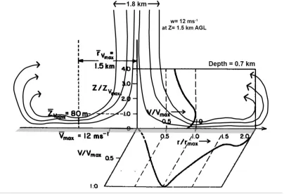
2008). A schematic of the velocity profile of downbursts from JAWS experiment is shown
in Figure 1.9. As can be seen in Figure 1.9, the maximum velocity in full scale and
experimental downburst is found around at a radius of approx. one downburst jet diameter
(Wilson et al., 1984; Hjelmfelt, 1988; Sengupta and Sarkar, 2008; McConville et al., 2009).
Figure 1.9: Velocity profile for a full scale event from JAWS experiment (Adapted
from Hjelmfelt, 1988)
Chay and Letchford (2002) used a small scale continuous impinging jet and suggested that
a characteristics ‘nose’ profile develops when the radial distance becomes 0.75 times the
jet diameter. The horizontal velocity reaches its maximum at the same distance as the jet
diameter. Similar results have been found from the experiments conducted by Mason et al.
Hangan (2007). The height of the peak downburst velocity increases with the increase in
radial distance (Wood et al., 2001; McConville et al., 2009). Recent experiments
McConville et al. (2009) and Zhang et al. (2013) confirmed the peak velocity of a
downburst occurring at 𝑅/𝐷≈1.
Vertical profiles of downburst flows near the ground are different from synoptic boundary
layer winds.
Figure 1.10 shows an example of normalized thunderstorm downburst velocity profile
compared with boundary layer winds (Kim and Hangan, 2007). Wood et al. (2001) also
investigated the velocity profiles of downbursts at different radial locations from the
downdraft centre. Similarities were found when compared with full scale data from JAWS
Figure 1.10: Comparison of downburst mean velocity profiles between empirical
model, laboratory experiment and typical boundary layer profiles (Adapted from
Kim and Hangan, 2007)
Aside from the three techniques (ring-vortex, cooling source and impinging jet) to simulate
downburst identified by Zhang et al. (2013), another approach, namely wall jets (also
referred to as slot jets), has also been adopted by researchers (Lin and Savory, 2006; Lin et
al., 2007; Lin and Savory, 2010). This technique employs a secondary strong flow through
a slot on the floor of traditional boundary layer wind tunnel to model the downburst outflow
(Lin and Savory, 2006). While they are relatively simple to implement and provide good
resolution in the surface region, these models do not reproduce the accurate vortex
structure, as they concentrate on generating vorticity through a wall jet mechanism. As a
result, the primary vortex structure lifts from the surface and does not produce a proper
dynamic separation reattachment (Mason et al., 2005). Impinging jet technique, where the
entire three dimensional flow structures of downbursts are modelled, provide better
simulations compared to wall jet technique (Lin and Savory, 2006).
In the present study, downbursts are simulated using an impinging jet technique at the
analyzes the downburst wind speed time history similar to an approach used for full scale
downburst records (Solari et al., 2015) as well as compares the important turbulence
characteristics (Spectra, probability density function, gust factor) relevant to wind loading
of structures with full scale downburst events. In addition, particle image velocimetry
(PIV) measurement technique is employed to analyze the vortex dynamics. Details of this
analysis is presented in Chapter 3 of this thesis.
1.5
Motivation and purpose of this thesis
Downbursts are highly transient in nature and therefore one of the primary targets of this
research is to investigate this transient nature using an objective method. A useful
methodology to analyze transient signals has been used previously by researchers
(Lavielle, 2005; Killick et al., 2012) for signal processing but never used on downburst
signals to separate thunderstorm period from mean ABL flow. In addition, time series
analysis is used to understand the typical downburst duration as well as the partition of full
scale downburst events based on a variety of events worldwide.
The current research also focuses on the characterization of the downbursts turbulent flow
field at high spatial and temporal resolutions. A large scale impinging jet approach is
employed, as it is the best compromise between reproducing the vortex dynamics
corresponding to real events and providing sufficient surface layer resolution. The large
scale WindEEE Dome at Western University (Hangan et al., 2017) is used to characterize
the turbulent flow field from simulated downbursts with high spatial and time resolution.
First, a time analysis of the velocity field is conducted based on Cobra probe measurements
and using a similar approach to full scale analysis previously conducted by Solari et al.
(2015). This allows the comparison of not only the mean but most importantly the
turbulence between full scale and experimental downbursts.
Secondly, a large scale PIV analysis is conducted in order to investigate the vortex
Considering all these different aspects, the following are the motivations of this thesis:
• To identify an objective method that can separate different stages of downbursts
from a thunderstorm time history record
• To analyze the transient characteristics of downburst events from different parts of the world to obtain a perception of downburst characteristics around the world
• To investigate the downburst characteristics for different flow and geometrical
parameters in an experimental simulator, which in turn would lead to recreating full
scale downburst events in a laboratory environment
• To analyze the downburst flow in the surface layer with comparison to ABL flow
• To characterize the statistical parameters of turbulence in a downburst and how
they relate to full scale downburst events
• To understand the structure and evolution of the primary downburst vortex and
compare it with available full scale data
1.6
Organization of this thesis
This thesis follows the ‘Integrated article’ format as per thesis submission requirement of
Western University. The thesis contains two articles described in Chapter 2 and Chapter 3
respectively.
Chapter 1 provides a brief introduction of thunderstorm downbursts and discusses the
previous projects capturing full scale data. This section also includes a review of downburst
characteristics obtained from laboratory experiments as well as numerical simulations by
previous researchers.
Chapter 2 presents and analyzes the full scale downburst events from 3 different continents:
Europe, US and Australia. 37 downburst records from 14 downburst events analyzed to
Chapter 3 focuses on the parametric characterization of large scale laboratory simulated
downbursts in the unique three dimensional wind testing chamber, the WindEEE Dome. A
moving time averaging method is employed to decompose the downburst time history for
wind engineering application following the criteria set by Holmes (2008) and Solari et al.
(2015). Turbulent characteristics and notable wind ratios (𝑅, 𝐺𝑚𝑎𝑥, 𝐺̂) from the downburst
flow are compared with previous full scale downburst events. Analysis on the primary
vortex structure (primary vortex formulation, vortex trajectory) were carried out by PIV
experiment explaining in the latter part of this chapter.
Chapter 4 provides the conclusions and an overall summary of the thesis. This section also
recommends the scope of future works from this current study.
1.7
References
Alahyari, A., Longmire, E.K., 1994. Particle image velocimetry in a variable density flow: application to a dynamically evolving microburst. Experiments in Fluids 17, 434– 440. https://doi.org/10.1007/BF01877047
Burlando, M., Romanić, D., Solari, G., Hangan, H., Zhang, S., 2017. Field Data Analysis and Weather Scenario of a Downburst Event in Livorno, Italy, on 1 October 2012. Monthly Weather Review 145, 3507–3527. https://doi.org/10.1175/MWR-D-17-0018.1
Byers, H.R., Braham, R.R., 1948. Thunderstorm structure and circulation. J. Meteor. 5, 71–86. https://doi.org/10.1175/1520-0469(1948)005<0071:TSAC>2.0.CO;2
Chay, M.T., Letchford, C.W., 2002. Pressure distributions on a cube in a simulated thunderstorm downburst—Part A: stationary downburst observations. Journal of Wind Engineering and Industrial Aerodynamics 90, 711–732. https://doi.org/10.1016/S0167-6105(02)00158-7
Chen, L., Letchford, C.W., 2004. A deterministic–stochastic hybrid model of downbursts and its impact on a cantilevered structure. Engineering Structures 26, 619–629. https://doi.org/10.1016/j.engstruct.2003.12.009
Choi, E.C.C., Hidayat, F.A., 2002. Gust factors for thunderstorm and non-thunderstorm winds. Journal of Wind Engineering and Industrial Aerodynamics, Fifth
Asia-Pacific Conference on Wind Engineering 90, 1683–1696.
Cook, N.J., Ian Harris, R., Whiting, R., 2003. Extreme wind speeds in mixed climates revisited. Journal of Wind Engineering and Industrial Aerodynamics 91, 403–422. https://doi.org/10.1016/S0167-6105(02)00397-5
Fujita, 1978. Manual of downburst identification for Project NIMROD. SMRP Res. Paper, 156 104.
Fujita, T., 1990. Downbursts: meteorological features and wind field characteristics. Journal of Wind Engineering and Industrial Aerodynamics, The Sixth U.S.
National Conference on Wind Engineering 36, 75–86.
https://doi.org/10.1016/0167-6105(90)90294-M
Fujita, T.T., 1985. The Downburst: Microburst and MacRoburst. University of Chicago.
Fujita, T.T., 1974. Jumbo Tornado Outbreak of 3 April 1974. Weatherwise 27, 116–126. https://doi.org/10.1080/00431672.1974.9931693
Fujita, T.T., Wakimoto, R.M., 1981. Five Scales of Airflow Associated with a Series of Downbursts on 16 July 1980. Mon. Wea. Rev. 109, 1438–1456. https://doi.org/10.1175/1520-0493(1981)109<1438:FSOAAW>2.0.CO;2
Gomes, L., Vickery, B.J., 1978. Extreme wind speeds in mixed wind climates. Journal of Wind Engineering and Industrial Aerodynamics 2, 331–344. https://doi.org/10.1016/0167-6105(78)90018-1
Gunter, W.S., Schroeder, J.L., 2015. High-resolution full-scale measurements of thunderstorm outflow winds. Journal of Wind Engineering and Industrial Aerodynamics 138, 13–26. https://doi.org/10.1016/j.jweia.2014.12.005
Hangan, H., Refan, M., Jubayer, C., Parvu, D., Kilpatrick, R., 2017. Big Data from Big Experiments. The WindEEE Dome, in: Whither Turbulence and Big Data in the 21st Century? Springer, Cham, pp. 215–230. https://doi.org/10.1007/978-3-319-41217-7_12
Hjelmfelt, M.R., 1988. Structure and Life Cycle of Microburst Outflows Observed in Colorado. J. Appl. Meteor. 27, 900–927. https://doi.org/10.1175/1520-0450(1988)027<0900:SALCOM>2.0.CO;2
Holmes, J.D., Hangan, H.M., Schroeder, J.L., Letchford, C.W., Orwig, K.D., 2008. A forensic study of the Lubbock-Reese downdraft of 2002. Wind and Structures 11, 137–152. https://doi.org/10.12989/was.2008.11.2.137
Holmes, J.D., Oliver, S.E., 2000. An empirical model of a downburst. Engineering Structures 22, 1167–1172. https://doi.org/10.1016/S0141-0296(99)00058-9
Järvi, L., Punkka, A.-J., Schultz, D.M., Petäjä, T., Hohti, H., Rinne, J., Pohja, T., Kulmala, M., Hari, P., Vesala, T., 2007. Micrometeorological observations of a microburst in southern Finland, in: Atmospheric Boundary Layers. Springer, New York, NY, pp. 187–203. https://doi.org/10.1007/978-0-387-74321-9_13
Jesson, M., Haines, M., Singh, N., Sterling, M., Taylor, I., 2013. Numerical and Physical Simulation of a Thunderstorm Downburst. Research Publishing Services, pp. 1139–1148. https://doi.org/10.3850/978-981-07-8012-8_P3
Jesson, M., Sterling, M., 2018. A simple vortex model of a thunderstorm downburst – A parametric evaluation. Journal of Wind Engineering and Industrial Aerodynamics 174, 1–9. https://doi.org/10.1016/j.jweia.2017.12.001
Killick, R., Fearnhead, P., Eckley, I.A., 2012. Optimal Detection of Changepoints With a Linear Computational Cost. Journal of the American Statistical Association 107, 1590–1598. https://doi.org/10.1080/01621459.2012.737745
Kim, J., Hangan, H., 2007. Numerical simulations of impinging jets with application to downbursts. Journal of Wind Engineering and Industrial Aerodynamics 95, 279– 298. https://doi.org/10.1016/j.jweia.2006.07.002
Landreth, C.C., Adrian, R.J., 1990. Impingement of a low Reynolds number turbulent circular jet onto a flat plate at normal incidence. Experiments in Fluids 9, 74–84. https://doi.org/10.1007/BF00575338
Lavielle, M., 2005. Using penalized contrasts for the change-point problem. Signal Processing 85, 1501–1510. https://doi.org/10.1016/j.sigpro.2005.01.012
Letchford, C.W., Chay, M.T., 2002. Pressure distributions on a cube in a simulated thunderstorm downburst. Part B: moving downburst observations. Journal of Wind
Engineering and Industrial Aerodynamics 90, 733–753.
https://doi.org/10.1016/S0167-6105(02)00163-0
Letchford, C.W., Mans, C., Chay, M.T., 2002. Thunderstorms—their importance in wind engineering (a case for the next generation wind tunnel). Journal of Wind Engineering and Industrial Aerodynamics, Fifth Asia-Pacific Conference on Wind Engineering 90, 1415–1433. https://doi.org/10.1016/S0167-6105(02)00262-3
Lin, W.E., Orf, L.G., Savory, E., Novacco, C., 2007. Proposed large-scale modelling of the transient features of a downburst outflow. Wind and Structures 10, 315–346. https://doi.org/10.12989/was.2007.10.4.315
Lin, W.E., Savory, E., 2010. Physical modelling of a downdraft outflow with a slot jet. Wind and Structures 13, 385–412. https://doi.org/10.12989/was.2010.13.5.385
Lin, W.E., Savory, E., 2006. Large-scale quasi-steady modelling of a downburst outflow
using a slot jet. Wind and Structures 9, 419–440.
Lombardo, F.T., Smith, D.A., Schroeder, J.L., Mehta, K.C., 2014. Thunderstorm characteristics of importance to wind engineering. Journal of Wind Engineering
and Industrial Aerodynamics 125, 121–132.
https://doi.org/10.1016/j.jweia.2013.12.004
Lundgren, T.S., Yao, J., Mansour, N.N., 1992. Microburst modelling and scaling. Journal of Fluid Mechanics 239, 461–488. https://doi.org/10.1017/S002211209200449X
Mason, M.S., Letchford, C.W., James, D.L., 2005. Pulsed wall jet simulation of a stationary thunderstorm downburst, Part A: Physical structure and flow field characterization. Journal of Wind Engineering and Industrial Aerodynamics 93, 557–580. https://doi.org/10.1016/j.jweia.2005.05.006
Mason, M.S., Wood, G.S., Fletcher, D.F., 2009. Numerical simulation of downburst winds. Journal of Wind Engineering and Industrial Aerodynamics 97, 523–539. https://doi.org/10.1016/j.jweia.2009.07.010
McConville, A.C., Sterling, M., Baker, C.J., 2009. The physical simulation of thunderstorm downbursts using an impinging jet. Wind and Structures An International Journal 12, 133–149. https://doi.org/10.12989/was.2009.12.2.133
McCullough, M., Kwon, D.K., Kareem, A., Wang, L., 2014. Efficacy of Averaging Interval for Nonstationary Winds. Journal of Engineering Mechanics 140, 1–19. https://doi.org/10.1061/(ASCE)EM.1943-7889.0000641
Orf, L.G., Oreskovic, C., Savory, E., Kantor, E., 2014. Circumferential analysis of a simulated three-dimensional downburst-producing thunderstorm outflow. Journal of Wind Engineering and Industrial Aerodynamics 135, 182–190. https://doi.org/10.1016/j.jweia.2014.07.004
Panneer Selvam, R., Holmes, J.D., 1992. Numerical simulation of thunderstorm downdrafts. Journal of Wind Engineering and Industrial Aerodynamics, Special Issue 8th International Conference on Wind Engineering 1991 44, 2817–2825. https://doi.org/10.1016/0167-6105(92)90076-M
Proctor, F.H., 1988. Numerical Simulations of an Isolated Microburst. Part I: Dynamics and Structure. J. Atmos. Sci. 45, 3137–3160. https://doi.org/10.1175/1520-0469(1988)045<3137:NSOAIM>2.0.CO;2
Schultz, T.A., 1990. Multiple vortex ring model of the DFW microburst. Journal of Aircraft 27, 163–168. https://doi.org/10.2514/3.45913
Sherman, D.J., 1987. The Passage of a Weak Thunderstorn Downburst over an
Instrumented Tower. Mon. Wea. Rev. 115, 1193–1205.
https://doi.org/10.1175/1520-0493(1987)115<1193:TPOAWT>2.0.CO;2
Solari, G., Burlando, M., De Gaetano, P., Repetto, M.P., 2015. Characteristics of thunderstorms relevant to the wind loading of structures. Wind and Structures 20, 763–791. https://doi.org/10.12989/was.2015.20.6.763
Srivastava, R.C., 1985. A Simple Model of Evaporatively Driven Dowadraft: Application to Microburst Downdraft [WWW Document].
http://dx.doi.org/10.1175/1520-0469(1985)042<1004:ASMOED>2.0.CO;2. URL
https://journals.ametsoc.org/doi/abs/10.1175/1520-0469(1985)042%3C1004:ASMOED%3E2.0.CO%3B2 (accessed 8.6.18).
Srivastava, R.C., Srivastava, R.C., 1987. A Model of Intense Downdrafts Driven by the Melting and Evaporation of Precipitation [WWW Document]. http://dx.doi.org/10.1175/1520-0469(1987)044<1752:AMOIDD>2.0.CO;2. URL
https://journals.ametsoc.org/doi/abs/10.1175/1520-0469(1987)044%3C1752:AMOIDD%3E2.0.CO;2 (accessed 8.6.18).
Vermeire, B.C., Orf, L.G., Savory, E., 2011. Improved modelling of downburst outflows for wind engineering applications using a cooling source approach. Journal of Wind
Engineering and Industrial Aerodynamics 99, 801–814.
https://doi.org/10.1016/j.jweia.2011.03.003
Wakimoto, R.M., 1985. Forecasting Dry Microburst Activity over the High Plains. Mon.
Wea. Rev. 113, 1131–1143.
https://doi.org/10.1175/1520-0493(1985)113<1131:FDMAOT>2.0.CO;2
Wakimoto, R.M., 1982. The Life Cycle of Thunderstorm Gust Fronts as Viewed with Doppler Radar and Rawinsonde Data. Mon. Wea. Rev. 110, 1060–1082. https://doi.org/10.1175/1520-0493(1982)110<1060:TLCOTG>2.0.CO;2
Wilson, J.W., Roberts, R.D., Kessinger, C., McCarthy, J., 1984. Microburst Wind Structure and Evaluation of Doppler Radar for Airport Wind Shear Detection. J. Climate
Appl. Meteor. 23, 898–915.
https://doi.org/10.1175/1520-0450(1984)023<0898:MWSAEO>2.0.CO;2
Wilson, J.W., Wakimoto, R.M., 2001. The Discovery of the Downburst: T. T. Fujita’s Contribution. Bulletin of the American Meteorological Society 82, 49–62. https://doi.org/10.1175/1520-0477(2001)082<0049:TDOTDT>2.3.CO;2
Wolfson, M.M., 1988. Characteristics of Microbursts in the Continental United States.
Xu, Z., Hangan, H., 2008. Scale, boundary and inlet condition effects on impinging jets. Journal of Wind Engineering and Industrial Aerodynamics 96, 2383–2402. https://doi.org/10.1016/j.jweia.2008.04.002
Yao, J., Lundgren, T.S., 1996. Experimental investigation of microbursts. Experiments in Fluids 21, 17–25. https://doi.org/10.1007/BF00204631