Pelee: A Real-Time Object Detection System on Mobile Devices

(1)

Scholarship@Western

Electronic Thesis and Dissertation Repository

4-5-2018 2:30 PM

Pelee: A Real-Time Object Detection System on Mobile Devices

Jun Wang

The University of Western Ontario

Supervisor Ling, Charles X.

The University of Western Ontario Graduate Program in Computer Science

A thesis submitted in partial fulfillment of the requirements for the degree in Master of Science © Jun Wang 2018

Follow this and additional works at: https://ir.lib.uwo.ca/etd

Part of the Artificial Intelligence and Robotics Commons

Recommended Citation Recommended Citation

Wang, Jun, "Pelee: A Real-Time Object Detection System on Mobile Devices" (2018). Electronic Thesis and Dissertation Repository. 5278.

https://ir.lib.uwo.ca/etd/5278

This Dissertation/Thesis is brought to you for free and open access by Scholarship@Western. It has been accepted for inclusion in Electronic Thesis and Dissertation Repository by an authorized administrator of

(2)

Abstract

There has been a rising interest in running high-quality Convolutional Neural Network (CNN)

models under strict constraints on memory and computational budget. A number of efficient

architectures have been proposed in recent years, for example, MobileNet, ShuffleNet, and

NASNet-A. However, all these architectures are heavily dependent on depthwise separable

convolution which lacks efficient implementation in most deep learning frameworks.

Mean-while, there are few studies that combine efficient models with fast object detection algorithms.

This research tries to explore the design of an efficient CNN architecture for both image

classi-fication tasks and object detection tasks. We propose an efficient architecture named PeleeNet,

which is built with conventional convolution instead. On ImageNet ILSVRC 2012 dataset,

our proposed PeleeNet achieves a higher accuracy by 0.6% and 11% lower computational cost

than MobileNet, the state-of-the-art efficient architecture. It is also important to point out that

PeleeNet is of only 66% of the size of MobileNet and 1/49 size of VGG.

We then propose a real-time object detection system on mobile devices. We combine PeleeNet

with Single Shot MultiBox Detector (SSD) method and optimize the architecture for fast speed.

Meanwhile, we port SSD to iOS and provide an optimized code implementation. Our proposed

detection system, named Pelee, achieves 70.9% mAP on PASCAL VOC2007 dataset at the

speed of 17 FPS on iPhone 6s and 23.6 FPS on iPhone 8. Compared to TinyYOLOv2, the

most widely used computational efficient object detection system, our proposed Pelee is more

accurate (70.9% vs. 57.1%), 2.88 times lower in computational cost and 2.92 times smaller in

model size.

Keywords: Real-time Object Detection, Convolutional Neural Network, Efficient

Architec-ture, Mobile Device, Embedded Vision

(3)

First and foremost, I would like to express my sincere gratitude to my supervisor Prof. Charles

X. Ling for the continuous support and guidance of my study and research. I would not be

able to complete this thesis without his instructions and help. Thanks are also given to my

col-leagues for their collaboration and valuable discussions. Especially my colcol-leagues, Xiang Li

and Shuang Ao, gave me so many insightful suggestions. Last but not least, my

acknowledge-ment and love go to my family: my parents Youku Wang and Fengqin Cao, my wife Li Sun

and my two lovely kids Alice and Daniel. Without their encouragement, continuous love and

support, I would not be able to pursue my study in Western University and finish this thesis.

My research is supported by Mitacs grant and scholarship from the School of Graduate Studies

in Western University. Special acknowledgement is also given to the open source community.

Without the excellent open source software and projects, I would not be able to complete this

thesis.

(4)

List of Figures

1.1 Scenarios of on-device artificial intelligence . . . 2

2.1 Image classification vs. object detection . . . 6

2.2 Training vs. inference . . . 7

2.3 Convolution layer . . . 8

2.4 Pooling layer . . . 9

2.5 Algorithm of Batch Normalization . . . 10

2.6 Inception model with dimension reduction . . . 11

2.7 High level diagram of ResNet architecture . . . 12

2.8 High level diagram of DenseNet architecture . . . 13

2.9 Deep compression - three stage compression pipeline . . . 14

2.10 Convolution with XNOR-bitcount . . . 14

2.11 Standard convolution filters vs. depthwise convolution filters . . . 15

2.12 High level diagram of Faster R-CNN architecture . . . 16

2.13 High level diagram of one-stage detector architecture . . . 17

3.1 A deep DenseNet with three dense blocks . . . 19

3.2 A dense block with 5 layers and growth rate 4 . . . 20

3.3 Two-way dense layer . . . 21

3.4 Structure of stem block . . . 22

3.5 Cosine learning rate annealing vs. step learning rate decay . . . 29

3.6 Comparison of different models on Stanford Dogs . . . 31

4.1 Architecture of SSD . . . 35

4.2 Default boxes and aspect ratios in SDD . . . 42

(9)

4.5 Data augmentation in SSD . . . 44

4.6 Average Precision on VOC 2007 . . . 45

4.7 Detection examples: TinyYOLOv2 vs. Pelee . . . 46

5.1 Workflow of CoreML . . . 52

(10)

List of Tables

3.1 Computational cost of bottleneck layer . . . 22

3.2 Overview of PeleeNet architecture . . . 24

3.3 Experimental configuration for PeleeNet . . . 26

3.4 Impact of different elements in DenseNet-41 . . . 27

3.5 Effects of different feature enhancement methods . . . 28

3.6 Results on Stanford Dogs . . . 30

3.7 Effects of various design choices and components on performance . . . 31

3.8 Results on ILSVRC 2012 . . . 32

4.1 Parameters of feature maps . . . 37

4.2 Training parameters of Pelee . . . 40

4.3 Effects of various design choices on performance . . . 41

4.4 Results on PASCAL VOC 2007 . . . 41

5.1 Benchmark of efficient classification models on ILSVRC 2012 . . . 49

5.2 Benchmark of efficient one-stage detector on VOC 2007 . . . 49

5.3 Benchmark of one-stage detector on VOC 2007 . . . 51

A.1 Architecture of DenseNet-41 . . . 60

(11)

Appendix A Architecture of DenseNet-41 . . . 59

Appendix B Merging BatchNorm Layer with Conv Layer . . . 61

Appendix C More Detection Examples: TinyYOLOv2 vs. Pelee . . . 62

(12)

Chapter 1 Introduction

This chapter briefly introduces the overall content of this thesis. The first section describes the source of motivation for this research. The second section is a short description of the major contributions of the research. The thesis outline is introduced in the end.

1.1 Motivation

Convolutional Neural Networks have evolved to be the state-of-the-art technique in computer vision. However, these algorithms are computationally intensive, which makes it difficult to deploy on embedded devices with limited hardware resources. Meanwhile, on-device Arti-ficial Intelligence (AI) is highly demanded in many real-world applications, e.g. robotics, self-driving car, Advanced Driver Assistance System (ADAS) and augmented reality (AR), etc.

The increasing needs of running high-quality CNN models under strict constraints on mem-ory and computational budget encourage the study on model acceleration and compression. Many innovative methods [13][40][41][16][29][8] have been proposed in recent years, which promotes on-device AI greatly. However, most of these papers mainly focus on classification tasks. There are few papers that combine model acceleration methods with fast object detection algorithms [15].

This study tries to explore the design of the efficient CNN architecture for both image classifi-cation tasks and object detection tasks. The reason for choosing object detection is that, from the practical perspective, object detection is a basic application scenario in the real world, con-sidering that multiple objects being in a picture is common. From the academic perspective, object detection task means more technical challenges than classification task, which not only

(13)

From Song presents Deep Learning Tutorial and Recent Trends at FPGA17, Monterey

Figure 1.1: Scenarios of on-device artificial intelligence

needs to judge the category of objects, but also gives the specific location of each object. It covers both the classification problem and the regression problem. The research results are able to provide strong evidences for other machine learning tasks.

1.2 Contributions

In summary, our main contributions are listed as follows:

We propose a variant of DenseNet [14] architecture called PeleeNet for mobile devices.

(14)

1.2. Contributions 3

key features of PeleeNet are:

• Two-Way Dense LayerWe use a 2-way dense layer to get different scales of receptive fields. One way of the layer uses a small kernel size (3x3), which is good enough to capture small-size objects. The other way of the layer uses a larger 5x5 kernel to learn visual patterns for large objects. To reduce computational cost, we follow the common practice of replacing 5x5 convolution with two stacked 3x3 convolution. (Fig. 3.3)

• Stem Block We design an cost efficient stem block before the first dense layer. The structure of stem block is shown on Fig. 3.4. This stem block can effectively improve the feature expression ability without adding computational cost too much - better than other more expensive methods, e.g., increasing channels of the first convolution layer or increasing growth rate.

• Dynamic Number of Channels in Bottleneck LayerAnother highlight is that the num-ber of channels in the bottleneck layer varies according to the input shape to make sure the number of output channels does not exceed the number of its input channels. Com-pared to the original DenseNet structure, our experiments show that this method can save up to 28.5% of the computational cost with a small impact on accuracy.

• Transition Layer without Compression Our experiments show that the compression factor proposed by DenseNet hurts the feature expression. We always keep the number of output channels the same as the number of input channels in transition layers.

• Composite FunctionWe use the conventional wisdom of post-activation (Convolution - Batch Normalization [17] - Relu) as our composite function instead of pre-activation used in DenseNet. For post-activation, all batch normalization layers can be merged with convolution layer at the inference stage, which can accelerate the speed greatly.

We optimize the network architecture of Single Shot MultiBox Detector (SSD) [26] for speed acceleration and then combine it with PeleeNet. Our proposed system, named Pelee, achieves 70.9% mAP on PASCAL VOC [3] 2007 object detection dataset. It also outperforms Tiny-YOLOv2 [31], the most widely used computational efficient object detection system, in terms of a higher accuracy by 13.8%, 2.88 times lower in computational cost and 2.92 times smaller in model size. The major enhancements proposed to balance speed and accuracy are:

• Feature Map Selection We build object detection network in a way different from the original SSD with a carefully selected set of 5 scale feature maps (19 x 19, 10 x 10, 5 x 5, 3 x 3, and 1 x 1). To reduce computational cost, we do not use 38 x 38 feature map.

(15)

• Small Convolutional Kernel for PredictionResidual prediction block makes it possible for us to apply 1x1 convolutional kernels to predict category scores and box offsets. Our experiments show that the accuracy of the model using 1x1 kernels is almost the same as that of the model using 3x3 kernels. However, 1x1 kernels reduce the computational cost by 21.5%.

We provide an efficient implementation of SSD algorithm on iOS. We have successfully ported SSD to iOS and provided an optimized code implementation. Our proposed system runs at the speed of 17.1 FPS on iPhone 6s and 23.6 FPS on iPhone 8. The speed on iPhone 6s, a phone released in 2015, is 2.6 times faster than that of the official SSD implementation on a server with a powerful Intel [email protected] CPU.

We provide a benchmark test for different efficient classification models and different one-stage object detection methods on NVIDIA GPU, Intel CPU and iPhone.

1.3 Thesis Outline

(16)

Chapter 2 Background

This chapter describes the background information related to this study. Section 2.1 and section 2.2 clarifies some key terminologies. Section 2.3 introduces the major layers of Convolutional Neural Network (CNN) and some popular network architectures. Section 2.4 briefly intro-duces datasets used in this study. The last section introintro-duces some previous work for network acceleration and object detection.

2.1 Image Classification vs. Object Detection

Image recognition/classification refers to predicting the label of an image among predefined labels. It assumes that there is single object of interest in the image and it covers a significant portion of image. Detection is about not only finding the class of object but also localizing the extent of an object in the image. The object can be lying anywhere in the image and can be of any size. (Fig. 2.1)

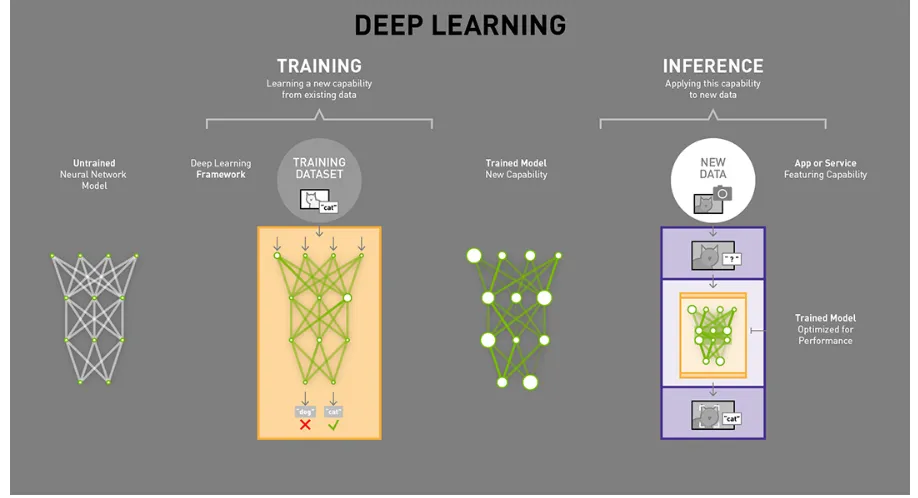
2.2 Training vs. Inference

Deep Learning is a most popular approach for learning representations. It has been widely used for all kinds of computer vision tasks and achieved state-of-the-art performance. On a high level, working with deep learning is a two-phase process: training and inference. Training is the phase in which a neural network tries to learn from the data. Inference is the phase in which a trained network is deployed to the product environment and is used to infer/predict the

(17)

From http://cs231n.stanford.edu/slides/2016/winter1516 lecture8.pdf

Figure 2.1: Image classification vs. object detection

new data.

There are different performance goals for training and inference. Usually people can tolerate a long training time to get a powerful model, but it is hoped that inference time should be as short as possible. Training can be sped up by using multiple GPUs in parallel with large batch size. However, inference typically batches a smaller number of inputs than training to meet the low latency requirement of AI-powered services. (Fig. 2.2)

2.3 Convolutional Neural Network

2.3.1 Layers in CNN

Convolutional Neural Networks (CNN) is one of the most popular deep learning methods. A CNN consists of different types of layers. Each layer has a simple work-flow: It transforms an input 3D volume to an output 3D volume with some differentiable function that may or may not have parameters. This section introduces some major layers used in our study.

Convolutional Layer

(18)

2.3. ConvolutionalNeuralNetwork 7

From https://blogs.nvidia.com/blog/2016/08/22/difference-deep-learning-training-inference-ai/

Figure 2.2: Training vs. inference

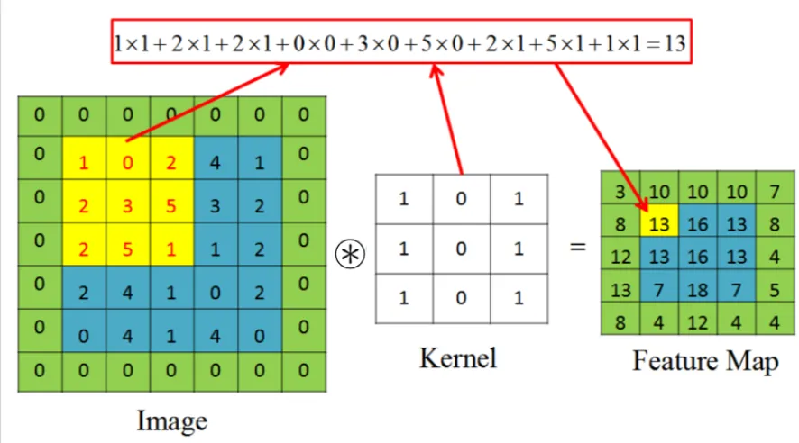
depth of the input volume. During the forward pass, each filter is convolved across the width and height of the input volume, computing the dot product between the entries of the filter and the input and producing a 2-dimensional activation map of that filter. (Fig. 2.3)

Relu Layer

ReLU is the abbreviation of Rectified Linear Units. This layer applies the non-saturating acti-vation function f(x) = max(0,x). It perfects the nonlinear properties of the decision function and of the overall network without affecting the receptive fields of the convolution layer.

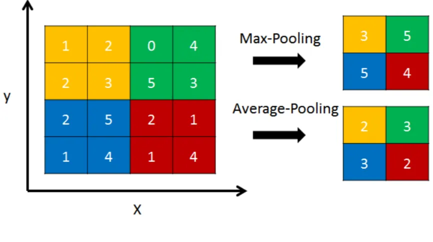
Pooling Layer

Another important layer of CNNs is pooling, which is a form of non-linear down-sampling. There are several non-linear functions to implement pooling among which max pooling and average pooling are the two most common. Max pooling partitions the input image into a set of non-overlapping rectangles and, for each such sub-region, outputs the maximum. (Fig. 2.4)

Batch Normalization Layer

(19)

Convolution operation with 3 x 3 kernel, stride 1 and padding 1._~denotes the convolutional operator

Figure 2.3: Convolution layer

2.3.2 Network Architecture

The first CNN that had a great success on image classification is the LeNet proposed by Y.LeCun in 1989 [23]. Its successor AlexNet [22] won ILSVRC challenge in 2012 and signifi-cantly outperformed the runner-up (top 5 error of 16% compared to runner-up with 26% error). After that many excellent network architectures have been proposed. This section lists some famous network architectures that are related to this research or have inspired our design.

VGGNet

(20)

2.3. ConvolutionalNeuralNetwork 9

Figure 2.4: Pooling layer

GoogLeNet

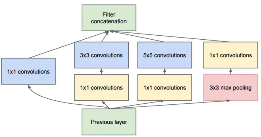
GoogLeNet, proposed by Szegedy et al. [37] from Google, is the ILSVRC 2014 winner. Its main contribution is the development of an Inception Module that dramatically reduces the number of parameters in the network. (Fig. 2.6)

ResNet

Residual Network (ResNet), proposed by Kaiming He et al. [9], is the winner of ILSVRC 2015 and COCO 2015. It features special skip connections to make training a very deep network easier. ResNet is currently by far the state of the art Convolutional Neural Network model and is widely used in all kinds of computer vision tasks. (Fig. 2.7)

DenseNet

(21)

Input :Values ofxover a mini-batch{x1...m}

Parameters to be learned: γ, β

Output:nyi = BNγ,β(xi)

o

µ← 1

m

X

i=1

xi //mini−batch mean

σ2 _← 1

m

X

i=1

(xi−µ)2 //mini−batch variance

ˆ xi ←

xi−µ

√

σ2+ //normalize

yi ←γxˆi+β //scale and shi f t

Figure 2.5: Algorithm of Batch Normalization

2.4 Datasets

Here we introduce datasets that are used in different tasks. ImageNet [2] ILSVRC 2012 and a customized Stanford Dogs [19] are used for image classification tasks. PASCAL VOC [3] 2007 and 2012 are used for object detection tasks.

2.4.1 ImageNet ILSVRC 2012

ImageNet [2] is an image dataset organized according to the WordNet hierarchy. Each mean-ingful concept in WordNet is called a ”synonym set” or ”synset”. ImageNet uses ”WordNet ID” (wnid) to uniquely identify a synset. For example, the wnid of synset ”dog, domestic dog, Canis familiaris” is ”n02084071”.

(22)

2.4. Datasets 11

From Going deeper with convolutions [37]

Figure 2.6: Inception model with dimension reduction

2.4.2 CIFAR-10

CIFAR-10 [21] is a popular toy image classification dataset. This dataset consists of 60,000 32x32 color images containing one of 10 object classes, with 6000 images per class. Although CIFAR-10 is widely used for ablation study, we do not use this dataset in this thesis. The main reason is that we have limited computing resource and hope that the hyper parameters got from ablation study can be used for ImageNet ILSVRC task. However, the hyperparameters used on CIFAR-10 are not able to be used on ILSVRC because CIFAR-10 is a low resolution dataset while ILSVRC is a high resolution dataset. Moreover, the network architectures on these two datasets are also different. Therefore, we build a customized Stanford Dogs dataset described as follows.

2.4.3 Stanford Dogs

Stanford Dogs [19] dataset contains images of 120 breeds of dogs from around the world. This dataset has been built using images and annotation from ImageNet for the task of fine-grained image classification.

(23)

From http://www.cs.cornell.edu/gaohuang/papers/DenseNet-CVPR-Slides.pdf

Figure 2.7: High level diagram of ResNet architecture

categories within entry level categories. We believe the dataset used for this kind of task is complicated enough to evaluate the performance of the network architecture. However, there are only 14,580 training images, with about 120 images per class, in the original Stanford Dogs dataset, which is not large enough to train the model from scratch.

Instead of using the original Stanford Dogs, we build a subset of ILSVRC 2012 according to the ImageNet wnid used in Stanford Dogs. Both training data and validation data are exactly copied from the ILSVRC 2012 dataset. In the following chapters, the term of Stanford Dogs means this subset of ILSVRC 2012 instead of the original one. Contents of this dataset:

• Number of categories: 120

• Number of training images: 150,466

• Number of validation images: 6,000

2.4.4 PASCAL VOC

PASCAL VOC [3] Challenge is a challenge in visual object recognition funded by PASCAL network of excellence. The datasets from the challenges are widely used for the benchmark of detection and segmentation tasks. The twenty object classes that have been selected are:

• Person: person

• Animal:bird, cat, cow, dog, horse, sheep

• Vehicle:aeroplane, bicycle, boat, bus, car, motorbike, train

(24)

2.5. RelatedWork 13

From http://www.cs.cornell.edu/gaohuang/papers/DenseNet-CVPR-Slides.pdf

Figure 2.8: High level diagram of DenseNet architecture

2.5 Related Work

2.5.1 Network Acceleration and Compression

The high computational cost and the large model size are two main factors restricting CNN being used on embedded systems. Researchers have worked great efforts to solve this problem in different ways.

Weights Pruning and Quantization

Song Han et al. propose deep compression, a three-stage pipeline: pruning, trained quantiza-tion and Huffman coding [8], to reduce the storage requirement of neural networks by 35x to 49x without affecting their accuracy. (Fig. 2.9)

Network Binarization

(25)

From Deep compression: Compressing deep neural networks with pruning, trained quantization and

huffman coding [8]

Figure 2.9: Deep compression - three stage compression pipeline

for ResNet-18, XNOR-Net is 18.1% lower in top-1 accuracy than the full precision network on ImageNet ILSVRC 2012 (51.2% vs 69.3%). (Fig. 2.10)

From Xnor-net:Imagenet classification using binary convolutional neural networks [29]

Figure 2.10: Convolution with XNOR-bitcount

Knowledge Distilling

Another approach is knowledge distillation [11][33] which trains a student network from the softened output of an ensemble of deeper and wider networks, called teacher network. The main idea is to allow the student network to capture not only the information provided by the true labels, but also the feature learned by the teacher network.

Efficient Network Architectures

Instead of depending on a large model, efficient architecture design tries to design and train a network from scratch to meet the strictly constraints budget.

(26)

2.5. RelatedWork 15

accuracy to VGG. Many of its outstanding design ideas have greatly affected the current net-work design. For example, S. Hong et al. [20] widely uses inception block in PVANet, which is a high accuracy real time object detection system.

MobileNet [13] is a pioneering work on efficient model architecture and for the first time shows the VGG level accuracy for a fully convolutional network with about 600 Million MACs (the number of Multiply-Accumulates which measures the number of fused Multiplication and Ad-dition operations) computational budget. MobileNet is based on a streamlined architecture that uses depthwise separable convolutions to build light weight CNNs. ShuffleNet [40] is another efficient model which utilizes pointwise group convolution and channel shuffle together with depthwise separable convolution to balance computational cost and accuracy. NASNet [41] is a complicated network obtained by reinforcement learning and model search. It achieves state of the art results both among large scale models and efficient models. NASNet architecture uses depthwise separable convolutions with different sizes ranging from 3x3 to 5x5, 7x7. However, the size of 7x7 is rarely used in human designed efficient models.

All these three famous efficient models heavily depend on depthwise separable convolution. Depthwise separable convolution is initially used in Inception models [37][38] to reduce the computation in the first few layers. Depthwise separable convolution is made up of two layers: depthwise convolution and pointwise convolution. Depthwise convolution applies a single filter per each input channel. Pointwise convolution is just a standard 1x1 convolution which is used to create a linear combination of the output of the depthwise layer. (Fig. 2.11)

(a) Standard convolution filters (b) Depthwise convolution filters

From http://machinethink.net/blog/googles-mobile-net-architecture-on-iphone/

(27)

2.5.2 Object Detection

Object detection is one of the main areas of researches in computer vision. Recent progress in object detection is heavily driven by the successful application of deep Convolutional Neural Networks (CNN). State-of-the-art CNN based object detection methods can be divided into two groups: region proposal-based detector and one-stage detector.

Proposal-based Detector

Proposal-based detector, also called two-stage detector, includes R-CNN [6], Fast RCNN [5], Faster R-CNN [32] and R-FCN [1]. There are two stages in proposal-based detector. Some potential object regions are generated at the first stage, and then classification and location processing are made on these proposed regions at the second stage. R-CNN uses selective search [39] to generate region proposal and then uses a CNN network to extract features from these proposed regions - each region is processed by the CNN network separately. Faster R-CNN improve the efficiency by sharing computation and using neural networks to generate the region proposals. (Fig. 2.12)

From Speed/accuracy trade-offs for modern convolutional object detectors [15]

Figure 2.12: High level diagram of Faster R-CNN architecture

One-stage Detector

(28)

2.5. RelatedWork 17

From Speed/accuracy trade-offs for modern convolutional object detectors [15]

Figure 2.13: High level diagram of one-stage detector architecture

Numerous excellent studies focus on pushing one-stage detection algorithms forward.

• YOLOv2 [31] proposes various improvements on YOLO detection method - both on speed and accuracy. YOLOv2 uses a lightweight backbone network called Darknet19 and a fully-convolutional architecture to accelerate the speed. By combining batch nor-malization, dimension clusters, anchor box and multi-scale training, YOLOv2 has im-proved the accuracy by up to 15% in mAP on VOC2007.

• DSSD [4], and Residual Feature and Unified Prediction Network (RUN) [24] improve the accuracy of SSD algorithm by optimizing the network structure of the detection parts. DSSD combines the deconvolutional layers with the existing multiple layers to reflect the large-scale context. RUN enriches the representation power of feature maps using multi-way residual block and unified prediction module. Deeply Supervised Object Detector (DSOD) [34] shows a high accuracy object detector can be trained without relying on Im-ageNet pre-training model when it combines a variant DenseNet architecture with SSD framework. However, these optimizations result in a much slower speed in comparison to the original SSD since more operations are added. Huang et al. [15] investigates var-ious combination of network structures and detection frameworks, and indicates that a detector combined SSD and MobileNet can achieve real time speeds and can be deployed on a mobile device.

(29)

PeleeNet: An E

ffi

cient Feature Extraction

Network

3.1 Introduction

Tremendous progress has been made in recent years on object detection due to the use of convolutional neural network (CNN). A CNN based object detector depends on a powerful feature extraction network. The feature extraction network directly affects memory, speed and performance of the detector. In SSD framework, over 90% of computation cost is consumed by the feature extraction network. In this chapter, we explore an architecture design for the efficient feature extraction network.

A number of efficient network architectures have been proposed in recent years, for exam-ple, MobileNet [13], ShuffleNet [40], and NASNet-A [41]. These models have been shown to achieve VGG level accuracy on ImageNet ILSVRC classification task with only 1/30 of theo-retical computational cost and model size. However, these models are heavily dependent on the depthwise separable convolution which lacks efficient implementation in most deep learning frameworks and hardware. Therefore, the actual speed is far less than the theoretical speed.

We propose a variant of DenseNet [14] architecture called PeleeNet which is built with con-ventional convolution operation instead. Our PeleeNet is designed to meet strict constraints on memory and computational budget. We propose the methods of two-way dense layer, stem block, transition layer without compression to improve the accuracy and also the methods of dynamic number of channels in bottleneck layer and post-activation to accelerate the speed. A series of controlled experiments on Stanford Dogs dataset and ImageNet ILSVRC 2012 dataset show the effectiveness of our design principles. Compared to the state-of-the-art architecture

(30)

3.2. Methodology 19

MobileNet, PeleeNet achieves a higher accuracy by 6.53% and 11% lower in computational cost on Stanford Dogs dataset (80.03% top-1) and a higher accuracy by 0.6% on ILSVRC 2012 dataset (71.3% top 1). Based on the DenseNet architecture, which is well known for encourag-ing feature reuse and substantially reducencourag-ing the number of parameters, our proposed PeleeNet is of only 66% of the model size of MobileNet.

3.2 Methodology

3.2.1 Review of DenseNet

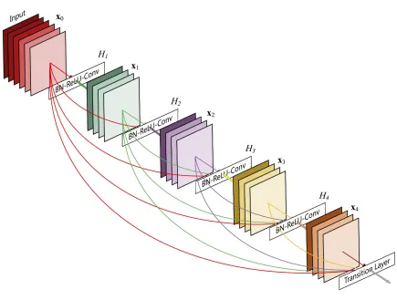
DenseNet [14] consists of multiple dense blocks, each of which consists of multiple dense layers. Each dense layer produces kfeatures, wherek is referred to as the growth rate of the network. The greatest contribution of DenseNet is that the input of each layer is a concatenation of all feature maps generated by all preceding layers within the same dense block. (Fig. 3.1 Fig. 3.2) Some other key points in DenseNet are:

Composite function. The composite function used in DenseNet consists of three consecutive operations: batch normalization (BN) [17], followed by a rectified linear unit (ReLU) [7] and a 3 x 3 convolution (Conv).

Bottleneck layers. Following the practice in [9][38], DenseNet uses a 11 convolution as bot-tleneck layer before each 33 convolution to reduce the number of input feature-maps, and thus to improve computational efficiency. Each bottleneck layer produces 4kfeature-maps (kis the growth rate).

Compression factor. Compression factorθ(range from 0 to 1 and default is 0.5) is introduced at transition layer to further improve model compactness. If a dense block containsmfeature maps, the following transition layer will generate [θ∗m] output feature maps. Whenθ=1, the number of feature-maps across transition layers remains unchanged.

(31)

Figure 3.2: A dense block with 5 layers and growth rate 4

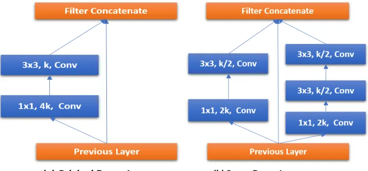
3.2.2 Two-Way Dense Layer

We use a 2-way dense layer to get different scales of receptive fields. One way of the layer uses a small kernel size (3x3), which is good enough to capture small-size objects. The other way of the layer uses a larger 5x5 kernel to learn visual patterns for large objects. To reduce the computational cost, we follow the common practice of replacing 5x5 convolution with two stacked 3x3 convolution [38]. The experimental results show that the 2-way dense layer achieves at least 2% higher accuracy on Stanford Dogs. (Fig. 3.3)

3.2.3 Stem Block

(32)

3.2. Methodology 21

Figure 3.3: Two-way dense layer

3.2.4 Dynamic number of Channels in Bottleneck Layer

Another highlight is that the number of channels in bottleneck layer varies according to the input shape to make sure the number of channels in bottleneck layer does not exceed the num-ber of its input channels. This method can effectively reduce the computational cost with little impact on the accuracy.

In DenseNet, the number of channels in the bottleneck layer is suggested to be 4 times the growth rate. Our experiments show that a larger bottleneck channels indicates a higher ac-curacy. However, a larger bottleneck channels also means an increasing computational cost. We observe that for the first layers, the number of bottleneck channels is much larger than the number of its input channels, which means that for these layers, bottleneck layer increases the computational cost instead of reducing the cost. As we can see from Table 3.1, for the first 4 layers, bottleneck layers increase about 3 times computational cost in total than the one without bottleneck layers. To maintain the consistency of the architecture, we still add the bottleneck layer to all dense layers, but the number is dynamically adjusted according to the input shape, to ensure that the number of channels does not exceed the input channels. Compared to a fixed 4-time-growth-rate scheme, the model with 4 time growth rate and dynamic scheme can reduce the computational cost by 28.5% with a small amount of loss of accuracy.

3.2.5 Transition Layer Without Compression

(33)

Input

1x1, 16, stride 1, conv

3x3, stride 2 max pool 3x3, 32, stride 2, conv

Filter concatenate

1x1, 32, stride 1, conv 56x56x32

56x56x64

112x112x32 3x3, 32, stride 2, conv

224x224x3

Figure 3.4: Structure of stem block

Dense Layer Input Channels

Computational Cost(Million MACs)

Fixed 4 x Without Bottleneck Layer Dynamic+4x

Layer 1 24 125 22 31

Layer 2 56 138 51 60

Layer 3 88 38 24 30

Layer 4 120 41 20 38

Total 342 117 159

Table 3.1: Computational cost of bottleneck layer

Dogs accuracy thanθ=0.5 .

3.2.6 Composite Function

We use the conventional wisdom of post-activation (Convolution - Batch Normalization - Relu) as our composite function instead of pre-activation (Batch Normalization - Relu - Convolution) used in DenseNet architecture. The main reason is not for accuracy but for the actual speed. For post-activation, all batch normalization layers can be merged with convolution layer at the inference stage, which can accelerate the speed greatly.

(34)

3.3. Experiments 23

He et al. [10] and has been proved to be able to effectively improve the performance of a very deep network. This method has made a significant contribution to DenseNet. Since DenseNet uses the concatenation operation to combine features, this method can achieve a unique scale and bias to previous features. For ResNet, there is no difference in the accuracy between the pre-activation and the post-activation when the depth of the model is less than 50. However, for DenseNet, pre-activation has a positive effect on both deep model and shallow model. Without pre-activation, the CIFAR-100 error of a 100-layer DenseNet grows from 22.27 to 24.30 [28]. Our experiments show that there is 0.92% lower accuracy on Stanford Dogs for a 41-layer DenseNet model without pre-activation.

Although this approach increases the accuracy, at least half of the batch normalization layers cannot be merged into the convolution layer to reduce the inference time. In consideration of this factor, in our architecture design, we use the traditional post-activation. To compensate for the negative impact caused by this change, we use a shallow and wide network structure. Meanwhile, a 2-way dense layer is used to improve the accuracy. We also add a 1x1 convolu-tion layer after the last dense block to get the stronger representaconvolu-tional abilities.

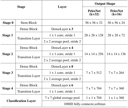
3.2.7 Overview of Architecture

Our proposed architecture is shown as follows in Table 3.2. The entire network consists of a stem block and four stages of feature extractor. Except the last stage, the last layer in each stage is average pooling layer with stride 2. A four-stage structure is a commonly used structure in the large model design. ShuffleNet et al. use three stage structure and shrink the feature map size at the beginning of each stage. Although this can effectively reduce computational cost, we argue that early stage features are very important for vision tasks, and that premature reducing the feature map size can impair representational abilities. Therefore, we still maintain a four-stage structure. The number of layers in the first two four-stages are specifically controlled to an acceptable range.

3.3 Experiments

3.3.1 Dataset

(35)

Stage Layer Output Shape PeleeNet

(k=32)

PeleeNet (k=16)

Stage 0 Stem Block 56 x 56 x 32 56 x 56 x 24

Stage 1

Dense Block DenseLayerx 3

28 x 28 x 128 28 x 28 x 72 Transition Layer 1 x 1 conv, stride 1

2 x 2 average pool, stride 2

Stage 2

Stage 3

Stage 4 Dense Block DenseLayerx 6 7 x 7 x 704 7 x 7 x 360

Transition Layer 1 x 1 conv, stride 1

Classification Layer 7 x 7 global average pool 1 x 1 x 704 1 x 1 x 360

1000D fully-connecte,softmax

Table 3.2: Overview of PeleeNet architecture

Since both training data and validation data are from counterparts in ILSVRC 2012 without any change, we can evaluate a model pre-trained on ILSVRC 2012 on this customized Stanford Dogs dataset. By this way, we can get some baseline information to help evaluate our model design. We have evaluated some pre-trained models, e.g. MobileNet, DenseNet121, VGG16 and ResNet50. The accuracy of the pre-trained MobileNet is 73.5%, which is slightly higher than the MobileNet model we trained from scratch (72.9%) on this dataset.

3.3.2 Evaluation

(36)

3.3. Experiments 25

highest probability answers must match the true label.

Accuracy= n−1

n

X

i=1

1(ˆyi−yi)

Cross Entropy Lossis a widely used loss function in classification problem. The true prob-ability pi is the true label, and the given distribution qi is the predicted value of the current

model. We can use cross entropy to get a measure for similarity between pandq:

H(p,q)=−X

x

p(x) logq(x)

Softmax Classifieris a widely used multi-class classifier in CNN. For softmax classifier, the cross-entropy loss is then given by:

Li =−log

          

ef_yi

P

j

efj           

or equivalentlyLi = −f_yi+logP j

efj _where _f

j(z)= e

z j P

k

ezk

3.3.3 Training Parameters

All models are trained by PyTorch, an open source machine learning library supported by Facebook. We follow most of the training settings and hyper-parameters used in ResNet on ILSVRC 2012 - except for the cosine learning rate decay policy used in section 3.3.6 and section 3.3.7.

3.3.4 Impact of Di

ff

erent Elements

We first evaluate the impact of the different elements (e.g., compress factor, bottleneck width, and pre-activation) of the dense block on accuracy and computational cost in order to support our decision making. We build a DenseNet-like network called DenseNet-41 as our baseline model. There are two differences between this model and the original DenseNet. The first one is the parameters of the first conv layer. There are 24 channels on the first conv layer instead of 64, the kernel size is changed from 7 x 7 to 3 x 3 as well. The second one is that the number of layers in each dense block is adjusted to meet the computational budget. The details of the architecture of DenseNet-41 can be seen at Appendix A.

(37)

Batch Size 256

Optimizer SGD

Learning Rate 0.1

Learning Rate Decay Policy Drop 0.1 every 30 epochs

Momentum 0.9

Weight Decay Rate 0.0001

Data Augmentation Random sized crop

Total Epochs 120

Table 3.3: Experimental configuration for PeleeNet

DenseNet architecture is a perfect fit for embedded vision. The basic DenseNet-41 model already presents a good performance. Its accuracy is 1.52% higher than the one of MobileNet (75.02 vs. 73.5) at similar computational cost.

The compression factor hurts the feature expression. When the compression ratio is changed from 0.5 to 1, the accuracy increases by 1.1% (from 75.02% to 76.12%) with 20% computa-tional cost increased as well.

Adjusting bottleneck channels is an effective way to balance computational cost and accuracy. Compared to the baseline model, when the number of bottleneck channel is changed to 3 times the growth rate and the compression factor is not applied, the accuracy increases by 0.45% (from 75.02% to 75.47%) with 5.3% less computation cost.

A larger bottleneck channels indicates a higher accuracy, but a larger bottleneck channels also means a increasing computational cost. For the channels with 3 times growth rate, the compu-tational cost is 21% less than the one with 4 times growth rate, but the accuracy is also reduced by 0.65%.

Pre-activation composite function makes a significant contribution to accuracy increase. The model with pre-activation composite function is 0.92% higher in accuracy than the one with post-activation.

(38)

3.3. Experiments 27 Model Dynamic bottleneck channels Million MACs Million Parameters Top-1 Accuracy

MobileNet N/A 569 4.24 73.5

DenseNet-41

(Bottleneck width=4x Compression=0.5)

7 543 1.07 75.02

DenseNet-41

7 652 1.57 76.12

DenseNet-41

Post-activation

7 652 1.57 75.2

DenseNet-41

(Bottleneck width=3x

Compression=1.0)

7 515 1.23 75.47

DenseNet-41

(Bottleneck width=4x

Compression=1.0)

3 466 1.49 75.75

Table 3.4: Impact of different elements in DenseNet-41

3.3.5 E

ff

ects of Di

ff

erent Feature Enhancement Methods

The second experiment compares different feature enhancement methods including the two-way dense layer, the stem block, increasing the number of dense layers and increasing the number of channels of the first convolution layer. All models are built with dynamic bottleneck channels scheme and without compression factor.

From Table 3.5, we can see that:

Stem block can effectively improve the accuracy. The result of stem block method is 0.87% higher in accuracy than the one without stem block. Stem block method outperforms the other two feature enhancement methods: increasing the channel of the first convolution layer and adding more dense layers. The result of stem block method is 0.82% higher in accuracy than the one of increasing the channel of the first convolution layer (76.57 vs. 75.75) and is 0.75% higher than the one of the method of adding more dense layers (76.57 vs. 75.82) , with much lower computational cost than these two methods.

(39)

model with two-way dense layer shows 2% higher accuracy than the one with one-way dense layer.

Early stage layers significantly increase accuracy. The accuracy increases by 0.55% when another dense layer added at stage 1.

No. Model Stem

Block 2-way Dense Layer Million MACs Million Parameters Top-1 Accuracy 1 DenseNet-41

(24-32-2466) 7 7 466 1.49 75.75

2 DenseNet-41

(36-32-2466) 7 7 517 1.55 75.75

3 DenseNet-45

(24-32-2486) 7 7 515 1.79 75.82

4 DenseNet-41

(24-32-2486) 3 7 502 1.5 76.57

5 DenseNet-45

(32-32-2486) 3 3 528 1.98 78.8

6 PeleeNet

(32-32-3486) 3 3 507 2.18 79.25 DenseNet-41(A−k−B) describes the network structure.Adenotes the number of channels in the first

convolution layer.kis the growth rate in dense blocks.Bdenotes the number of dense layer in each dense block.

Table 3.5: Effects of different feature enhancement methods

3.3.6 Results on Stanford Dogs

This section describes the result on Stanford Dogs and the result compared to other pre-trained models. We use a different data augmentation method in this section. Besides random-sized cropping, we also randomly adjust brightness and contrast of training images. This new data augmentation approach brings a 0.3% performance boost. Different from previous sections, the model is trained with a cosine learning rate annealing schedule (PeleeNet cosine), similar to what is used by [28][27].

(40)

3.4. Summary 29

(a) Learning rate decay (b) Accuracy

Figure 3.5: Cosine learning rate annealing vs. step learning rate decay

Based on the results of the above experiments, the effects of various design choices on the per-formance can be summarized as Table 3.7. After combining all these design choices, PeleeNet achieves 80.03% accuracy on Stanford Dogs, which is 5.01% higher in accuracy than the base-line DenseNet-41 at less computational cost.

3.3.7 Results on ILSVRC 2012

As we can see from Table 3.8, PeleeNet achieves a compelling result on ILSVRC 2012. PeleeNet is 0.6% more accurate than MobileNet and 0.4% more accurate than ShuffleNet.

3.4 Summary

DenseNet architecture is well suited for computing constrained scenarios. Because of its in-novative connectivity pattern, the features can be effectively reused to build an efficient model without depthwise separable convolution.

(41)

Model Million MACs

Million

Parameters

Top-1

Accuracy

VGG16 15,346 14.71 75.45

ResNet50 3,832 23.48 79.48

DenseNet-121 2,833 6.87 78.65

1.0 MobileNet 569 3.32 73.5

PeleeNet (k=32) 507 2.18 79.55

PeleeNet (k=32)- cosine 507 2.18 80.03

0.5 MobileNet 150 1.34 66.8

PeleeNet (k=16) 150 0.55 75.2

Table 3.6: Results on Stanford Dogs

PeleeNet is good at the fine-grained image recognition. It achieves the state of the art result on Stanford Dogs dataset. The top 1 accuracy is 80.03%, which is 6.53% higher than that of MobileNet. This accuracy is even higher than that of DenseNet-121 and ResNet50. Moreover, the computational cost of PeleeNet is only 18.6% of the cost of DenseNet-121 and only 13.7% of the one in ResNet50.

(42)

3.4. Summary 31

(a) Computational cost (b) Model size

Figure 3.6: Comparison of different models on Stanford Dogs

From DenseNet-41 to PeleeNet

Transition layer

with-out compression 3 3 3 3 3 3 3 3

Post-activation ₃ ₃ ₃ ₃ ₃

Dynamic bottleneck

channels 3 3 3 3 3 3

Stem Block 3 3 3 3 3

Two-way dense layer ₃ ₃ ₃ ₃

Go deeper ₃ ₃ ₃

Extra data

augmenta-tion 3 3

Cosine learning rate

annealing 3

Top 1 accuracy 75.02 76.1 75.2 75.8 76.8 78.8 79.25 79.55 80.03

(43)

Model Million MACs

Million

Parameters

Top-1

Accuracy

Top-5

Accuracy

VGG16 15,346 14.71 71.5 89.8

ResNet50 3,832 23.48 75.9 93.0

DenseNet-121 2,833 6.87 75.0 92.3

1.0 MobileNet 569 4.24 70.7 89.5

ShuffleNet 2x (g=3) 524 5.2 70.9

-NASNet-A 564 5.3 74.0 91.6

PeleeNet (k=32) 508 2.8 71.3 90.3

(44)

Chapter 4 Pelee: A Real-Time Object Detection

System

4.1 Introduction

Considering the compelling speed advantage of the one-stage detection algorithms, we build our object detection system based on SSD [26] algorithm. Compared with YOLO [30] [31] series, the multi-scale feature maps used in SSD is a more efficient way to perform prediction. SSD with a 300 x 300 input size achieves better results than the 416 x 416 YOLOv2 [31] counterpart.

This chapter introduces our object detection system and the optimization for SSD. The main purpose of our optimization is to improve the speed with acceptable accuracy. Due to the time limitation, we mainly focus on the network architecture design. Our network structure can be combined with other optimization methods to further improve the accuracy in the future.

A number of enhancements have been proposed to manage a balance between speed and accu-racy. Except for our efficient backbone network proposed in last chapter, we also build feature extraction network in a way different from the original SSD with a carefully selected set of 5 scale feature maps. In the meantime, we follow the design ideas of RUN [24] that encourages features to be passed along the feature extraction network. For each feature map used for detec-tion, we build a residual block before conducting prediction. We also use small convolutional kernels to predict object categories and bounding box locations to reduce computational cost. In addition, we use quite different training hyperparameters.

Although these contributions may seem small independently, we note that the final system

(45)

achieves 70.9% mAP on VOC 2007, which is 13.4% higher in accuracy than TinyYOLOv2 (57.1% mAP). Compared with TinyYOLOv2, the system is also 2.88 times lower in computa-tional cost and 2.92 times smaller in model size.

4.2 Methodology

4.2.1 Review of SSD

SSD [26] is based on a feed-forward convolutional network that produces a fixed-size collec-tion of bounding boxes and scores for the presence of object class instances in those boxes. A non-maximum suppression step is used after this network to produce the final detection. Some key features of SSD are listed as follows:

Multi-scale Feature Maps for Detection

As it shows on Fig. 4.1, SSD adds convolutional feature layers, which decrease in size pro-gressively, to the end of the backbone network. These extra layers together with some layers of the backbone network can detect object at multiple scales, which is different from YOLO [30] that only operates on a single scale feature map. There are 6 different scale of feature maps used for predicting: 38 x 38, 19 x 19, 10 x 10, 5 x 5, 3 x 3, 1 x 1.

Default Boxes and Aspect Ratios

SSD associates a set of default bounding boxes with each feature map cell. SSD predicts the offsets of each default box shape, as well as the per-class scores that indicate the presence of a class instance in each of those boxes. Specifically, for each box out ofkat a given location, SSD computescclass scores and the 4 offsets relative to the original default box shape. This results in a total of (c+4)×k×m×noutputs for am×nfeature map.

(46)

4.2. Methodology 35

Figure 4.1: Architecture of SSD

Training Objective

The overall objective loss function in SSD is a weighted sum of the localization loss (loc) and the confidence loss (conf):

L(x,c,l,g)= 1

N(Lcon f(x,c)+αLloc(x,l,g))

where N is the number of matched default boxes. If N=0, the loss is set to 0.

The localization loss is a Smooth L1 loss between the predicted box (l) and the ground truth box (g) parameters.

Lloc(x,l,g)= N

X

i∈Pos

X

m∈{cx,cy,w,h}

xi jksmoothL1(lmi −gˆ m

j)

where

ˆ gcxj = (g

cx

j −d

cx

i )/d

w

i gˆ

cy

j =(g

cy

j −d

cy i )/d

h i

ˆ

gw_j = log(g

w j

dw i

) gˆh_j =log(g

h j

dh i

(47)

The confidence loss is the softmax loss over multiple classes confidences (c ).

Lcon f(x,c)= −

N

X

i∈Pos

x_{i j}plog(ˆc_ip)−

N

X

i∈Neg

log(ˆc0_i)

where ˆc_ip= exp(c

p i) P

pexp(c p i)

Hard Negative Mining

In SSD, after the matching step, most of the default boxes are negative samples, especially when the number of possible default boxes is large. This introduces a significant imbalance between the positive and negative training examples. The hard-negative mining is used to keep the ratio between the negatives and positives at most 3:1. Hard negative mining is the processing that all default boxes are sorted by the confidence loss and only the highestNboxes are selected as the negatives. This leads to faster optimization and a more stable training.

4.2.2 Feature Map Selection

There are 5 scales of feature maps used in our system for prediction: 19 x 19, 10 x 10, 5 x 5, 3 x 3, and 1 x 1. We do not use 38 x 38 feature map layer to ensure a balance able to be reached between speed and accuracy.

The 38 x 38 feature map has been shown to have a great positive impact on network accuracy in large scale models. For example, the accuracy of the SSD model with 38 x 38 feature map is 1.8% higher than that without 38 x 38 feature map on VOC2007. Our experiments also show that the RUN model with 38 x 38 feature map achieves 4.1% higher accuracy than the one without 38 x 38 feature map in VOC2007 (78.3% vs 74.2%).

(48)

4.2. Methodology 37

Original SSD SSD+MobileNet[15] Pelee

Prediction 1

Feature Map Size 38 x 38 19 x 19 19 x 19

Default Box Size 30 60 30.4

Aspect Ratio [1, 2, 1/2] [1, 2, 1/2] [1, 2, 1/2, 3, 1/3]

Prediction 2

Aspect Ratio [1, 2, 1/2, 3, 1/3] [1, 2, 1/2, 3, 1/3] [1, 2, 1/2, 3, 1/3]

Prediction 3

Aspect Ratio [1, 2, 1/2, 3, 1/3] [1, 2, 1/2, 3, 1/3] [1, 2, 1/2, 3, 1/3]

Prediction 4

Aspect Ratio [1, 2, 1/2, 3, 1/3] [1, 2, 1/2, 3, 1/3] [1, 2, 1/2, 3, 1/3]

Prediction 5

Aspect Ratio [1, 2, 1/2] [1, 2, 1/2, 3, 1/3] [1, 2, 1/2, 3, 1/3]

Prediction 6

Aspect Ratio [1, 2, 1/2] [1, 2, 1/2, 3, 1/3] [1, 2, 1/2, 3, 1/3]

Table 4.1: Parameters of feature maps

4.2.3 Residual Prediction Block

We follow the design ideas of RUN [24] and insert a two-way residual block (ResBlock) for each level of feature maps to separate and decouple the backbone network and the prediction module.

(49)

decouple backbone network from the prediction module. This approach clearly differentiates the features to be used for prediction from those to be delivered to the next layer. Moreover, it can prevent the gradient of the prediction module from flowing directly into the feature map of the backbone network. To meet our computational budget, we only use two-way ResBlock. (Fig. ??)

4.2.4 Small Convolutional Kernel for Prediction

We apply 1x1 convolutional kernels instead of 3x3 convolutional kernels used in original SSD to predict category scores and box offsets. Since our feature maps are built with two-way residual blocks, which have extracted the nearby features from the raw feature maps, 1x1 kernels are capable enough for conducting prediction. Our experiments show that the accuracy of the model using 1x1 kernels is almost same as the one of the model using 3x3 kernels. However, 1x1 kernels reduce the computational cost by 21.5%.

4.3 Experiments

4.3.1 Dataset

The proposed method is evaluated on PASCAL VOC 2007 and PASCAL VOC 2012 dataset. Following the common practice, we use VOC 2007 train+val data and VOC 2012 train+val data as our training data and VOC 2007 test data as our validation data set. There are about 16.5K training images in total.

4.3.2 Evaluation

Bounding Box Evaluation

For detection, a common way to determine if one object proposal is right isIntersection over Union (IoU). Detections are assigned to ground truth objects and are judged to be true/false positives by measuring bounding box overlap. To be considered a correct detection, the overlap ratio IoU between the predicted bounding box Bp and ground truth bounding box Bgt must

exceed 0.5 (50%) based on the formula

(50)

4.3. Experiments 39

whereBp∩Bgt denotes the intersection of the predicted and ground truth bounding boxes and

Bp∪Bgt their union.

Mean Average Precision (mAP)

The interpolated average precision (Salton and Mcgill 1986) is used on VOC2007 to evaluate detection [3]. For a given class, the precision/recall curve can be computed. Recall is defined as the proportion of all positive examples ranked above a given rank. Precision is the proportion of all examples above that rank which are from the positive class. The AP summarizes the shape of the precision/recall curve, and is defined as the mean precision at a set of eleven equally spaced recall levels [0,0.1,...,1]:

mAP= 1 11

X

r∈{0,0.1...,1)

Pinter p(r)

The precision at each recall levelris interpolated by taking the maximum precision measured for a method for which the corresponding recall exceedsr

Pinter p(r)=maxp(˜r)

˜

r:˜r≥r

where p(˜r) is the measured precision at recall ˜r.

Presision=

P

T ruePositive

P

T ruePositive+P

FalsePositive

Recall=

P

T ruePositive

P

T ruePositive+P

FalseNegative

True Positive: a proposal is made for classcand it actually is an object of classc.

False Positive: a proposal is made for classc, but it is not an object of classc.

False Negative: a proposal is made for non-classc, but it actually is an object of classc.

4.3.3 Data Augmentation

We follow the data augmentation strategies used in SSD. Each training image is randomly sampled by one of the following options (Fig. 4.5):

• Use the entire original input image.

• Sample a patch that the IoU with the target object is of 0.1, 0.3, 0.5, 0.7, or 0.9.

(51)

• Randomly expand a sampled image.

The size of each sampled patch is [0.1, 1] of the original image size, and the aspect ratio is between 1/2 and 2. The overlapped part of the ground truth box will be kept if the center of it is in the sampled patch. After the sampling step, each sampled patch is re-sized to a fixed size and is horizontally flipped with probability of 0.5, in addition to applying some photo-metric distortions similar to those described in [12].

4.3.4 Training Parameters

Our codes are based on the source codes of SSD1_{and are trained with Ca}ff_{e [18]. The training}

parameters are listed as follows. Our batch size and learning rate decay policy are different from the original SSD’s.

Batch Size 128

Optimizer SGD

Learning Rate 0.02

Learning Rate Decay Policy Drop 0.1 at 20,000 and 25,000 iterations

Momentum 0.9

Weight Decay Rate 0.0005

Total Iterations 40,000

Table 4.2: Training parameters of Pelee

4.3.5 Results on PASCAL VOC 2007

It can be seen from Table 4.3 and Table 4.4 that:

• The 38 x 38 feature map does not have an huge influence on accuracy. The model using 38 x 38 feature map achieves 0.7 % higher accuracy than the model without using 38 x 38 feature map (69.3 vs. 68.6) at 24.6% more computational cost.

• Residual prediction block can effectively improve the accuracy and does not increase computational cost too much. The model with residual prediction block achieves 70.6

(52)

4.4. Summary 41

% mAP, which is 2.0% higher in accuracy than the model without residual prediction block.

• The accuracy of the model using 1x1 kernels for prediction is almost same as the one of the model using 3x3 kernels. However, 1x1 kernels reduce the computational cost by 21.5% and the model size by 33.9%.

38x38 Feature ResBlock Kernel Size

For Prediction

Million MACs

Million

Parameters mAP

3 7 3x3 1670 5.69 69.3

7 7 3x3 1340 5.63 68.6

7 3 3x3 1470 7.27 70.8

7 3 1x1 1210 5.43 70.9

Table 4.3: Effects of various design choices on performance

Detection Frameworks Million MACs Million Parameters mAP (Larger is better)

Tiny-YOLOv2 3490 15.86 57.1

YOLOv2-288 7940 57.96 69.0

SSD+MobileNet 1150 5.78 68

Pelee 1210 5.43 70.9

Table 4.4: Results on PASCAL VOC 2007

4.4 Summary

(53)

Figure 4.2: Default boxes and aspect ratios in SDD

(54)

4.4. Summary 43

(a) ResBlock (b) Network of Pelee

(55)

Original image

Randomly cropped

and distorted sample Flipped and distorted sample Sample with IoU

Sample with IoU Randomly expanded sample

Flipped and randomly expanded sample

(56)

4.4. Summary 45

(57)

TinyYOLOv2 Pelee

Compared to TinyYOLOv2, our proposed Pelee can correctly detect sofa and also localize all

kinds of objects in the image correctly.More detection examples can be seen on Appendix C.

(58)

Chapter 5 Benchmark on Real Devices

5.1 Introduction

Counting MACs (the number of multiply-accumulates) is widely used to measure the compu-tational cost. However, it cannot replace the speed test on real devices, considering that there are many other factors that may influence the actual time cost, e.g. caching, I/O, hardware optimization etc,.

This chapter evaluates the performance of efficient models on mobile phones and the perfor-mance of several one-stage object detection models on CPU and GPU. We only evaluate the speed. The accuracy information originates from the related peer-reviewed paper and the pre-vious experiments. It is assumed that the model conversion will not result in reduced accuracy.

5.2 Benchmark on Mobile Phone

We evaluate the speed of some efficient classification models, including MobileNet and our proposed PeleeNet, on ImageNet ILSVRC 2012 and the speed of some efficient object de-tection models, including Tiny-YOLOv2, SSD + MobileNet and ours, on VOC 2007. All the models are directly converted from Caffe models without any model specific optimization being done.

The speed is calculated by the average time of processing 100 pictures. We run 100 picture processing for 10 times separately and average the time. For object detection models, the time reported here includes the image pre-processing time, but it does not include the time of the post

(59)

processing part (decoding the bounding-boxes and performing non-maximum suppression). Usually post processing is done on the CPU, which can be executed asynchronously with pre-processing and pre-processing that are executed on mobile GPU. Hence, the actual speed should be very close to our test result.

Our results are tested on iPhone 6s and iPhone 8. Apple iPhone 6s is a phone released in September of 2015. Its hardware capability is the same as or lower than the mainstream smart phone and embedded vision devices. Apple iPhone 8 is released in September of 2017, which is equipped with the state of the art hardware and the dedicated neural network hardware accel-erator. We choose iPhone as our test equipment, mainly because with the CoreML toolchains, a trained machine learning model can be easily converted and integrated into the iOS applica-tion. CoreML is a foundational machine learning framework used in Apple products, which features fast performance and easy integration. (Fig. 5.1)

5.2.1 Benchmark of E

ffi

cient Classification Model on ILSVRC 2012

It can be seen from Table 5.1 that:

On iPhone 6s, our proposed model runs at a similar speed as MobileNet, although our model indicates 11% lower computational cost. The reason may be that MobileNet is a streamlined shallow and wide model with about 27 convolutional layers, while our model is a multi-branch and narrow model with 113 convolutional layers. Shallow models are easier to be paralleled for more efficient execution. We try another shallow model named PeleeNet-shallow (32-32-3443). It has almost the same architecture as PeleeNet. The only difference is that the last two dense blocks have half number of dense layers with doubled growth rate (78 convolutional layers in total). PeleeNet-shallow runs faster than MobileNet and PeleeNet, although it has a higher computational cost than PeleeNet.

Models on iPhone 8 are about 25% to 30% faster than those on iPhone 6s. MobileNet runs almost the same speed as PeleeNet-shallow on iPhone 8.

5.2.2 Benchmark of E

ffi

cient One-stage Detector on VOC 2007

It can be seen from Table 5.2 that:

(60)

5.3. Benchmark onCPUandGPU 49

Model Million

MACs

Million

Parameters

Accuracy Speed(ms/image)

Top-1 Top-5 iPhone6s iPhone8

1.0 MobileNet 569 4.24 70.7 89.5 47.3 36.0

PeleeNet (k=32) 508 2.8 71.3 90.3 47.5 38.3

PeleeNet-shallow

(32-32-3443) 542 2.1 - - 44.3 35.8

Table 5.1: Benchmark of efficient classification models on ILSVRC 2012

Model Million

MACs

Million

Parameters

mAP Speed(FPS)

iPhone6s iPhone8

Tiny-YOLOv2[31] 3490 15.86 57.1 9.3 23.8

SSD+MobileNet[15] 1150 5.77 68 16.1 22.8

Pelee 1210 5.43 70.9 17.1 23.6

Table 5.2: Benchmark of efficient one-stage detector on VOC 2007

5.3 Benchmark on CPU and GPU

This section evaluates the performance of some one-stage detectors on NVIDIA GTX 1080 Ti GPU and Intel i7-6700K @ 4.00GHz CPU. All models are converted to Caffe [18] models and evaluated by Caffe time tool. With the exception of DSOD, the batch normalization layers of other models have been merged into the convolution layers. The speed on Titan X GPU are quoted from related papers. The results of the column 1080 Ti and Intel i7 are tested by our experiments.

It can been seen from Table 5.3 that:

(61)

The performance of MobileNet heavily depends on an efficient implementation of depthwise separable convolution. Under the same hardware and deep learning framework, there is about 9 times of gap in speed between cuDNN v5.0 and cuDNN v7.0. SSD+MobileNet [15] reaches 212 FPS on cuDNN v7.0 while only 24 FPS on cuDNN v5.0. The performance on cuDNN v5.0 is much slower than other efficient models’.

On CPU, both our proposed model and SSD+MobileNet run at about 6 FPS, which are 1.5 times faster than Tiny-YOLOv2. All high accuracy models (mAP > 76%) on CPU run at a speed slower than 1 FPS.

It is unexpected that the actual speed of the efficient models on iPhone is much faster than that on a powerful desktop CPU. The speed of TinyYOLOv2 on iPhone 6s is 2.8 times faster than that on Intel i7-6700K. Both SSD+MobileNet and our proposed model can run at a 1.6 times faster speed on iPhone 6s than on Intel i7-6700K.