End to end Network for Twitter Geolocation Prediction and Hashing

End-to-end Network for Twitter Geolocation Prediction and Hashing

Jey Han Lau1,2 _{Lianhua Chi}1 _{Khoi-Nguyen Tran}1 _{Trevor Cohn}2

1_{IBM Research}

2_{School of Computing and Information Systems,} The University of Melbourne

[email protected],[email protected],

[email protected],[email protected]

Abstract

We propose an end-to-end neural network to predict the geolocation of a tweet. The network takes as input a number of raw Twitter metadata such as the tweet mes-sage and associated user account informa-tion. Our model is language independent, and despite minimal feature engineering, it is interpretable and capable of learning location indicative words and timing pat-terns. Compared to state-of-the-art sys-tems, our model outperforms them by 2%-6%. Additionally, we propose extensions to the model to compress representation learnt by the network into binary codes. Experiments show that it produces com-pact codes compared to benchmark hash-ing algorithms. An implementation of the model is released publicly.1

1 Introduction

A number of applications benefit from geographi-cal information in social data, from personalised advertising to event detection to public health studies. Sloan et al.(2013) estimate that less than 1% of tweets are geotagged with their locations, motivating the development of geolocation predic-tion systems.

Han et al. (2012) introduced the task of pre-dicting the location based only the tweet mes-sage. A key difference to previous work is that the prediction is made at message or tweet level, while predecessor methods tend to focus on user-level prediction (Backstrom et al., 2010; Cheng et al., 2010). Since then, various methods have been proposed for the task (Han et al.,2014;Chi et al.,2016;Jayasinghe et al.,2016;Miura et al.,

1_{https://github.com/jhlau/} twitter-deepgeo

2016), although most systems are engineered for a particular platform and language (e.g. website-specific parsers and language-website-specific tokenisers and gazetteers). Another strand of research lever-ages the social network structure to infer location;

Jurgens et al.(2015) provided a standardised com-parison of these systems. Our focus in this pa-per is on using only the tweets, althoughRahimi et al.(2015) showed that the best approach maybe to combine both types of information.

In applications where fast retrieval of co-located tweets is necessary (e.g. disaster detection), effi-cient representation of large volume of tweets con-stitute an important issue. Traditionally, hashing techniques such as locality sensitive hashing ( In-dyk and Motwani,1998) are used to compress data into binary codes for fast retrieval (e.g. with multi-index hash tables (Norouzi et al.,2012,2014)), but it is not immediately clear how they can interact with raw Twitter metadata — as they often require a vector as input — and incorporate supervision.2

To this end, we propose an end-to-end neu-ral network for tweet-level geolocation prediction. Our network is designed to be interpretable: we show it has the capacity to automatically learn lo-cation indicative words and activity patterns from different regions.

Our contribution in this paper is two-fold. First, our model outperforms state-of-the-art systems by 2-6%, even though it has minimal feature engi-neering and is completely language-independent, as it uses no gazetteers or language preprocess-ing tools such as tokenisers or parsers. Second, our network can further compress learnt represen-tations into compact binary code that incorporates information about the tweet and its geolocation. To the best of our knowledge, this is the first end-to-end hashing method for tweets.

2_{In our case, the supervised information is the geolocation}

of tweets.

2 Related Work

Early work in geolocation prediction operated at the user-level. Backstrom et al. (2010) devel-oped a methodology to predict the location of a user on Facebook by measuring the relation-ship between geography and friendrelation-ship networks, andCheng et al.(2010) proposed a content-based prediction system to predict a Twitter user’s lo-cation based purely on his/her tweet messages.

Han et al. (2012) introduced tweet-level predic-tion, where they first extract location indicative words by leveraging the geotagged tweets and then train a classifier for geolocation prediction using the location indicative words as features. Extend-ing on this, systems were developed to better rank these location indicative or geospatial words by lo-cality (Chang et al.,2012;Laere et al.,2014;Han et al.,2014). More recently,Han et al.(2016) pro-posed a shared task for Twitter geolocation predic-tion, offering a benchmark dataset on the task.

Hashing is an effective method to compress data for fast access and analysis. Broadly there are two types of hashing techniques: data-independent techniques which design arbitrary functions to generate hashes, and data-dependent techniques that leverage pairwise similarity in the training data (Chi and Zhu,2017). Locality-sensitive hash-ing (lsh:Indyk and Motwani(1998)) is a widely-known data-independent hashing method that uses randomised projections to generate hashcodes. It preserves data characteristics and guarantees the collision probability between data points. fasthash(Lin et al.,2014), on the other hand, is a supervised data-dependent hashing that incorpo-rates label information to determine pairwise sim-ilarity. It uses decision tree based hash functions and graph cut-based binary code inference to deal with high dimensionality training data.

3 Geolocation Prediction

3.1 Dataset

We use the geolocation prediction shared task dataset (Han et al., 2016) for our experiments. There are 2 proposed tasks, predicting geolocation given: (1) a tweet (tweet-level); and (2) a collec-tion of tweets by a user (user-level). For each task, there is a hard classification evaluation setting for predicting a city class, and a soft evaluation setting for predicting latitude and longitude coordinates.

We explore only the more challenging

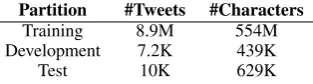
tweet-Partition #Tweets #Characters

Training 8.9M 554M

Development 7.2K 439K

Test 10K 629K

Table 1: Dataset statistics.

level prediction task. In terms of evaluation set-ting, we experiment with the hard classification setting, where the network is required to predict one out of 3362 cities. Note that the metadata of a tweet includes not only the message but a vari-ety of information such as creation time and user account data such as location and timezone.

Training, development and test partitions are provided by the shared task organisers.3 _We

pre-process the data minimally, removing tweets that have less than 5 characters in the training parti-tion (development and testing data is untouched) and keeping all character types that have occurred 5 times or more in training. Unseen character to-kens are represented by <UNK>. Preprocessed statistics of the dataset is given in Table1.

3.2 Network Architecture

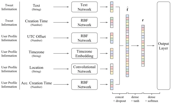
The overall architecture of our model (henceforth deepgeo) is illustrated in Figure 1. deepgeo uses 6 features from the metadata: (1) tweet mes-sage; (2) tweet creation time; (3) user UTC offset; (4) user timezone; (5) user location; and (6) user account creation time.4

Each feature from the metadata is processed by a separate network to generate a feature vectorfj. These feature vectors are then concatenated (with dropout applied) and connected to the penultimate layer:

ˆ

f =f1⊕f2...⊕fN (1)

r=tanh(Wrˆf) (2) whereNis the number of features (6 in total),r∈

RR_{is the hidden representation at the penultimate} layer andWris model parameter. For brevity, we omit biases in equations.

ris fully connected to the output layer and ac-tivated by softmax to generate a probability distri-bution over the classes. The model is trained with 3_{The organisers provide full metadata for the test}

parti-tion but only the tweet IDs for training and development par-titions. We collect metadata for training/development tweets using the Twitter API.

4_{We also tested user description and username, but}

Figure 1: Overall architecture ofdeepgeo.

minibatches and optimised using Adam (Kingma and Ba,2014) with standard cross-entropy loss.

We design several networks for the raw features. The first is a character-level recurrent convolu-tional network with a self-attention component for processing the tweet message (Section3.2.1). The second is an RBF network5 _{for processing}

num-bers (Section3.2.2). The third is a simple convo-lutional network for processing user location (Sec-tion3.2.3), and the last is an embedding matrix for user timezone. We treat the timezone as a categor-ical feature, and learn embeddings for each time-zone (309 unique timetime-zones in total). Note that these feature-processing networks are disjointed and there is no parameter sharing between them.

3.2.1 Text Network

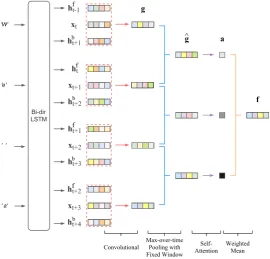
For the tweet message, we use a character-level recurrent convolutional network (Lai et al.,2015), followed by max-over-time pooling with a fixed window size and an attentional component to gen-erate the feature vector, as illustrated in Figure2.

Letxt∈REdenote the character embedding of the t-th character, we run a bi-directional LSTM network (Hochreiter and Schmidhuber, 1997) to generate the forward and backward hidden states

hf_t andhb

trespectively.6 We then concatenate the left and right context’s hidden states withxt and

5_{Also known as mixture density network.}

6_{LSTM is implemented using one layer without any}

peep-hole connections and forget biases are initialised with 1.0.

generate:

ˆ

xt=hft−1⊕xt⊕hbt+1

gt=ReLU(Wgˆxt)

wherexˆt ∈ R3E, Wg ∈ RO×3E and gt ∈ RO. We iterate for each character to generategtfor all time steps (Wg can be interpreted asO convolu-tional filters each with a window of3×E strid-ing 3 steps at a time). Next, we apply max-over-time (narrow) pooling with window size P over the vectors:

ˆ

gt=max(gt,gt+1, ...,gt+P−1)

wheregˆt∈ROand max is a function that returns the element-wise maxima given a number of vec-tors of the same length. If there areT characters in the tweet, this yields(T−P+1) ˆgvectors, one for each span.

By settingP =T, we could generate one vector for the whole tweet. The idea of using a smaller window is that it enables a self-attention compo-nent, thereby allowing the network to discover the saliency of a character span — for our task this means attending to location indicative words (Sec-tion3.4). We define the attention network as fol-lows:

αt=v|tanh(Wvgˆt)

a=softmax(α0, α1, ..., αT−P)

Figure 2: Text Network.

to generate the final feature vector:

ftext=

T_X−P

t=0

atgˆt

whereatdenotes thet-th element ina, andftext∈

RO_.

3.2.2 RBF Network

There are three time features in the metadata: tweet creation time, user account creation time and user UTC offset. The creation times are given in UTC time (i.e. not local time), e.g. Thu Jul 29 17:25:38 +0000 2010and the offset is an integer. For the creation times, we use only time of the day information (e.g.17:25) and normalise it from 0 to 1.7 _{UTC offset is converted to hours and}

nor-malised to the same range.8

The aim of the network is to split time into mul-tiple bins. We can interpret each hour as one bin (24 bins in total) and tweets originated from a par-ticular location (e.g. Europe) favour certain hours or bins. This preference of bins should be dif-ferent to tweets from a distant location (e.g. East Asia). Assuming each bin follows a Gaussian dis-tribution, then the goal of the network is to learn

7_{As an example,17:25is converted to 0.726.}

8_{UTC offset minimum is assumed -12 and maximum}

+14 based on: https://en.wikipedia.org/wiki/ List_of_UTC_time_offsets.

the Gaussian means and standard deviations of the bins.

Formally, given an input valueu, for binithe network computes:

ri= exp

−(u−µi)2

2σ2

i

whereri is the output value andµiandσi are the parameters for bini. LetB be the total number of bins, the feature vector generated by a RBF net-work is given as follows:

frbf= [r0, r1, ..., rB−1]

wherefrbf∈RB.

3.2.3 Convolutional Network

Location is a user self-declared field in the meta-data. As it is free-form text, we use a stan-dard character-level convolution neural network (Kim, 2014) to process it. The network architec-ture is simpler compared to the text network (Sec-tion 3.2.1): it has no recurrent and self-attention layers, and max-over-time pooling is performed over all spans.

use convolutional filters and max-over-time (nar-row) pooling to compute the feature vector:

gt=ReLU(Wgxt:t+Q−1)

fconv=max(g0,g1, ...,gT−Q)

whereQis the length of the character span,Wg∈ RO×QE _(W

g can be interpreted as O convolu-tional filters each with a window of Q×E) and

gt,fconv∈RO.

3.3 Experiments and Results

We explore two sets of features for predicting ge-olocation, using: (1) only the tweet message; and (2) both tweet and user metadata. For the latter ap-proach, we have 6 features in total (see Figure1). Classification accuracy is used as the metric for evaluation.

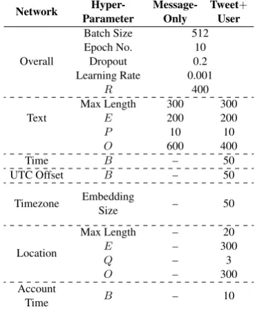
We tune network hyper-parameter values based on development accuracy; optimal hyper-parameter settings are presented in Table2. The column “Message-Only” uses only the text con-tent of tweets, while “Tweet+User” incorporates both tweet and user account metadata.

For tweet message and user location, the maxi-mum character length is set to 300 and 20 charac-ters respectively; strings longer than this threshold are truncated and shorter ones are padded.9

Mod-els are trained using 10 epochs without early stop-ping. In each iteration, we reset the model’s pa-rameters if its development accuracy is worse than that of previous iteration.

We compare deepgeo to 3 benchmark sys-tems, all of which are systems submitted to the shared task (Han et al.,2016):

Chi et al. (2016) propose a geolocation pre-diction approach based on a multinomial naive Bayes classifier using a combination of automati-cally learnt location indicative words, city/country names, #hashtags and @mentions. A frequency-based feature selection strategy is used to select the optimal subset of word features.

Miura et al. (2016) experiment with a simple feedforward neural network for geolocation clas-sification. The network draws inspiration from fastText (Joulin et al., 2016), where it uses mean word vectors to represent textual features and has only linear layers. To incorporate multiple 9_{Tweets can exceed the standard 140-character limit due}

to the use of non-ASCII characters.

Network _ParameterHyper- Message- Tweet_{Only User}+

Overall

Batch Size 512

Epoch No. 10

Dropout 0.2

Learning Rate 0.001

R 400

Text Max LengthE 300200 300200

P 10 10

O 600 400

Time B – 50

UTC Offset B – 50

Timezone Embedding_Size – 50

Location

Max Length – 20

E – 300

Q – 3

O – 300

Account _{B – 10}

Time

Table 2:deepgeohyper-parameters and values.

Accuracy System Features

0.146 Chi et al.(2016) Message Only

0.212 deepgeo Message Only 0.409 Miura et al.(2016) Tweet+User Metadata

0.428 deepgeo Tweet+User Metadata

0.436 Jayasinghe et al.(2016)

Tweet+User Metadata, Gazetteer, URL IP Lookup, Label Prop. Network

Table 3: Geolocation prediction test accuracy.

features — tweet message, user location, user de-scription and user timezone — the network com-bines them via vector concatenation.

Jayasinghe et al. (2016) develop an ensemble of classifiers for the task. Individual classifiers are built using a number of features indepedently from the metadata. In addition to using information em-bedded in the metadata, the system relies on exter-nal knowledgebases such as gazetteer and IP look up system to resolve URL links in the message. They also build a label propagation network that links connected users, as users from a sub-network are likely to come from the same location. These classifiers are aggregated via voting, and weights are manually adjusted based on development per-formance.

en-Tweet _LabelTrue Predicted_Label 1st Span 2nd Span 3rd Span

Big thanks to @LouSnowPlow and all #CleanSidewalk participants today. You really make Louisville shine. To be happy, be compassionate!

louisville-ky111-us louisville-ky111-us ‘Louisville’ ‘ake Louisv’ ‘ Louisvill’

McDonald’s with aldha (@ Jalan A. P. Pettarani)

http://t.co/HDVkhsKWBa makassar-38-id makassar-38-id ‘Pettarani)’ ‘ Pettarani’ ‘ettarani) ’ Let’s miss ALL the green lights on purpose! - every

driver in Moncton this morning moncton-04-ca halifax-07-ca ‘in Moncton’ ‘ncton this’ ‘Moncton th’ Harrys bar toilet selfie @sophiethielmann @

Carluc-cio’s Newcastle https://t.co/rKT7RGe7Nd newcastle upontyne-engi7-gb newcastle upontyne-engi7-gb ‘s Newcastl’ ‘wcastle ht’ ‘castle htt’

Makan terossssssss wkwkwk (with Erwina and Indah at

McDonald’s Bintara) - https://t.co/lT3KERFgap bekasi-30-id bekasi-30-id ‘ Bintara) ’ ‘ntara) - h’ ‘intara) - ’ @EileenOttawa For better or worse it’s a revenue

stream for Twitter made available to businesses. We all

have to get used to it. toronto-08-ca ottawa-08-ca ‘tawa For b’ ‘ttawa For ’ ‘nOttawa Fo’ Hunt work!! (with @hadiseptiandani and

@Febrianti-vivi at Jobforcareer Senayan) - https://t.co/u9myRDidtR jakarta-04-id jakarta-04-id ‘nayan) - h’ ‘ Senayan) ’ ‘enayan) - ’

Table 4: Examples of top character spans. Length of span is 10 characters. “1st Span” denotes the span that has the highest attention weight, “2nd Span” and “3rd Span” the second and third highest weight respectively.

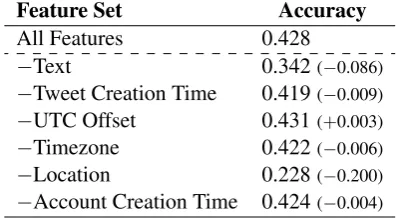
Feature Set Accuracy All Features 0.428

−Text 0.342(−0.086)

−Tweet Creation Time 0.419(−0.009)

−UTC Offset 0.431(+0.003)

−Timezone 0.422(−0.006)

−Location 0.228(−0.200)

−Account Creation Time 0.424(−0.004)

Table 5: Feature ablation results.

gineering and is trained at character level. Next, we compare deepgeo to Miura et al. (2016). Both systems use a similar set of features from the tweet and user metadata. deepgeo sees an encouraging performance, with almost 2% im-provement. The best system in the shared task,

Jayasinghe et al. (2016), remains the top per-former. Note, however, that their system de-pends on language-specific processing tools (e.g. tokenisers), website-specific parsers (e.g. for ex-tracting location information from user profile page on Instagram and Facebook) and external knowledge sources (e.g. gazetteers and IP lookup) which were inaccessible by other systems.

To better understand the impact of each fea-ture, we present ablation results where we remove one feature at a time in Table5. We see that the two most important features are the user location and tweet message. These observations reveal that self-declared user location appears to be a reliable source of location, as task accuracy drops by al-most half when this feature is excluded. For the other features, they generally have a small or

neg-ligible impact.

3.4 Qualitative Analyses

The self-attention component in the text net-work (Section3.2.1) captures saliency of charac-ter spans. To demonstrate its effectiveness, we se-lect a number of tweets from the test partition and present the top-3 spans that have the highest atten-tion weights in Table4.

Interestingly, we see that whenever a location word is in the message,deepgeotends to focus around it (e.g. Louisville andNewcastle). Occa-sionally this can induce error in prediction, e.g. in the second last example the network focuses onOttawaeven though the word has little signifi-cance to the true location (Toronto). Focussing on the right span does not necessarily result in correct prediction as well; as we see in the third exam-ple the network focuses onMonctonbut predicts a neighbouring cityHalifaxas the geolocation.

Next, we look at the Gaussian mixtures learnt by the RBF network. Using the gold-standard city labels, we collect bin weights (frbf) for tweet

cre-ation times (from test data) for 6 cities and plot them in Figure3. Each Gaussian distribution rep-resents one bin, and its weight is computed as a mean weight over all tweets belonging to the city (line transparency indicates bin weight). Bins that have a mean weight<0.075are excluded.

For London (Figure3c), we see that most tweets are created from 10:00–20:00 local time.10 _For

Jakarta (Figure3e), tweet activity mostly centers around 11:00–23:00 local time (04:00–16:00 UTC 10_{London’s UTC offset is +00 so no adjustment is}

00:00 04:00 08:00 12:00 16:00 20:00 24:000 5

10 15 20

25 rio de janeiro-21-br

(a) UTC-03

00:00 04:00 08:00 12:00 16:00 20:00 24:000 5

10 15 20

25 los angeles-ca037-us

(b) UTC-07

00:00 04:00 08:00 12:00 16:00 20:00 24:000 5

10 15 20

25 city of london-enggla-gb

(c) UTC+00

00:00 04:00 08:00 12:00 16:00 20:00 24:000 5 10 15 20 25 istanbul-34-tr (d) UTC+03

00:00 04:00 08:00 12:00 16:00 20:00 24:000 5 10 15 20 25 jakarta-04-id (e) UTC+07

00:00 04:00 08:00 12:00 16:00 20:00 24:000 5

10 15 20

25 kuala lumpur-14-my

(f) UTC+08

Figure 3: Tweet creation time distribution for 6 cities. Times in all plots are in UTC time. Sub-caption indicates a city’s UTC offset.

1.0 0.5 0.0 0.5 1.0 0 50000 100000 150000 200000 250000 300000 350000 400000

(a) 100; 0.0; 0.0

1.0 0.5 0.0 0.5 1.0 0 50000 100000 150000 200000 250000 300000 350000 400000

(b) 100; 0.1; 0.0

1.0 0.5 0.0 0.5 1.0 0 50000 100000 150000 200000 250000 300000 350000 400000

(c) 100; 0.0; 0.1

1.0 0.5 0.0 0.5 1.0 0 100000 200000 300000 400000 500000 600000 700000 800000

(d) 200; 0.0; 0.0

1.0 0.5 0.0 0.5 1.0 0 100000 200000 300000 400000 500000 600000 700000 800000

(e) 200; 0.1; 0.0

1.0 0.5 0.0 0.5 1.0 0 100000 200000 300000 400000 500000 600000 700000 800000

(f) 200; 0.0; 0.1

1.0 0.5 0.0 0.5 1.0 0 200000 400000 600000 800000 1000000 1200000

(g) 300; 0.0; 0.0

1.0 0.5 0.0 0.5 1.0 0 200000 400000 600000 800000 1000000 1200000

(h) 300; 0.1; 0.0

1.0 0.5 0.0 0.5 1.0 0 200000 400000 600000 800000 1000000 1200000

(i) 300; 0.0; 0.1

1.0 0.5 0.0 0.5 1.0 0 200000 400000 600000 800000 1000000 1200000 1400000 1600000

(j) 400; 0.0; 0.0

1.0 0.5 0.0 0.5 1.0 0 200000 400000 600000 800000 1000000 1200000 1400000 1600000

(k) 400; 0.1; 0.0

1.0 0.5 0.0 0.5 1.0 0 200000 400000 600000 800000 1000000 1200000 1400000 1600000

(l) 400; 0.0; 0.1 Figure 4: Histogram ofrelement values. Fields in the subcaptions denote vector dimension (R), corrup-tion level (σ) andlscaling factor (α). Range of y-axis for the same vector dimension is standardised.

time). Most cities share a similar activity period, with the exception of Istanbul (Figure3d): Turk-ish people seems to start their day much later, as tweets begin to appear from 15:00–01:00 local time (12:00 to 22:00 UTC time).

Another interesting trend we find is that for two cities (Los Angeles and Kuala Lumpur), there is a brief period of inactivity around noon (12:00) to evening (18:00) in local time. We hypothesise that most people are working during these times, and are thus too busy to use Twitter.

4 Hashing: Generating Binary Code For Tweets

deepgeocreates a low-dimensional dense vector representation (r) for a tweet in the penultimate

layer. This representation captures the message, user timezone and other metadata (including the city label) that are incorporated to the network dur-ing traindur-ing.

Storing the dense vector representation for a large volume of tweets can be costly.11 _{If we}

can compress the dense vectors into compact bi-nary codes, it would save storage space, as well as enabling more efficient retrieval of co-located tweets, e.g. using multi-index hash tables for K -nearest neighbour search (Norouzi et al., 2012,

2014).

Inspired by denoising autoencoders (Yu et al.,

2016;Vincent et al.,2010), webinarisethe dense

11_{If a tweet is represented by a vector of 400 32-bit floating}

Bits deepgeo deepgeo deepgeo_{+noise +loss word2vec deepgeo word2vec deepgeo}lsh fasthash

100 0.147 0.149 0.146 0.013 0.053 0.116 0.140

200 0.143 0.143 0.140 0.019 0.072 0.128 0.160

300 0.136 0.137 0.141 0.021 0.082 0.133 0.165

400 0.132 0.135 0.136 0.022 0.086 0.135 0.170

Table 6: Retrieval MAP performance.

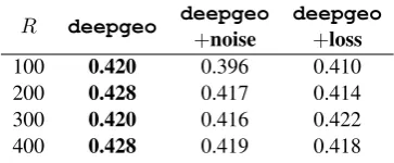
R deepgeo deepgeo deepgeo_{+noise +loss} 100 0.420 0.396 0.410 200 0.428 0.417 0.414 300 0.420 0.416 0.422 400 0.428 0.419 0.418

Table 7: Classification performance fordeepgeo with the addition of noise and loss terml.

vector generated by deepgeo by adding Gaus-sian noise. The intuition is that the addition of noise sharpens the activation values in order to counteract the random noise.

Equation (1) is thus modified to: ˆf = (f1 ⊕

f2...⊕fN) +N(0, σ2), whereN(0, σ2)is a zero-mean Gaussian noise with standard deviation (or corruption level)σ.12

In the addition to the Gaussian noise, we also experiment with an additional loss term l to pe-nalise elements that are not in the extrema: l = α× 1

R

P_R−1

i=0 |(ri −1)(ri + 1)|, whereri is the

i-th element inrandα is a scaling factor. We set

σ = α = 0.1, as both values were found to pro-vide good performance.

To better understand the effectiveness of the noise and loss term l in binarising the vector values, we present a histogram plot of r ele-ment values from test data in Figure4, for R = 100,200,300,400. We see that the addition of noise andlhelps in pushing the elements to the ex-trema. The noise term appears to work a little bet-ter thanl, as the frequency for the−1.0and+1.0

bins is higher. We also observe that there is a small increase in middle/zero values as R increases from 100 to 400, suggesting that there are more un-used hidden units when number of parameters in-creases. We present classification accuracy perfor-mance when we add noise (deepgeo+noise) andl(deepgeo+loss) in Table7. The perfor-mance drops a little, but generally stays within a gap of 1%. This suggests that both noise and l

12_{Dropout is applied toˆf, i.e. after the addition of noise.}

works well in binarisingrwithout trading off clas-sification accuracy significantly.

Next we evaluate the retrieval performance us-ing the binary codes. We binarise r for devel-opment and test tweets using the sign function. Given a test tweet, we retrieve the nearest devel-opment tweets based on hamming distance, and calculate average precision.13 _{We aggregate the}

retrieval performance for all test tweets by com-puting mean average precision (MAP).

For comparison, we experiment with two hash-ing techniques: lsh (Indyk and Motwani,1998) andfasthash(Lin et al.,2014) (see Section2

for system descriptions). The input required for bothlsh andfasthashis a vector. We test 2 types of input for these methods: (1) aword2vec baseline, where we concatenate mean word vec-tors of the tweet message, user account’s time-zone and location, resulting in a 900-dimension vector;14_{and (2)deepgeorepresentationr. The}

rationale for using deepgeo as input is to test whether its representation can be further com-pressed with these hashing techniques.15

We present MAP performance for all systems in Table 6. Looking at deepgeosystems (col-umn 2–4), we see that adding noise and l helps, although the impact is greater when the bit size is large (300/400 bits). Forlsh, which uses no la-bel information,word2vecinput produces poor binary code for retrieval. Changing the input to deepgeoimproves retrieval considerably, imply-ing that the representation produced bydeepgeo captures geolocation information.

fasthashwithword2vecinput vector per-forms competitively. For smaller bit sizes (100 or 200), however, the gap in performance is substan-13_{We remove 1328 test tweets that do not share city labels}

with any development tweets.

14_{300-dimensionword2vec(skip-gram) vectors are}

trained on English Wikipedia.

15_{lshandfasthashare trained using 400K tweets due}

tial. Pairingfasthashwithdeepgeoproduces the best retrieval performance: for 200/300/400 bits it outperformsdeepgeo+noise by 2–4%. Interestingly for 100 bitsfasthashis unable to compressdeepgeo’s representation any further, highlighting the compactness ofdeepgeo repre-sentation for smaller bit sizes.

5 Conclusion

We propose an end-to-end method for tweet-level geolocation prediction. We found strong perfor-mance, outperforming comparable systems by 2-6% depending on the feature setting. Our model is generic and has minimal feature engineering, and as such is highly portable to problems in other domains/languages (e.g. Weibo, a Chinese social platform, is one we intend to explore). We propose simple extensions to the model to compress the representation learnt by the network into binary codes. Experiments demonstrate its compression power compared to state-of-the-art hashing tech-niques.

References

L. Backstrom, E. Sun, and C. Marlow. 2010. Find me if you can: improving geographical prediction with social and spatial proximity. InProceedings of the 19th international conference on World wide web, pages 61–70. ACM.

H. Chang, D. Lee, M. Eltaher, and J. Lee. 2012. @ phillies tweeting from philly? predicting twitter user locations with spatial word usage. InProceedings of the 2012 International Conference on Advances in Social Networks Analysis and Mining (ASONAM 2012), pages 111–118. IEEE Computer Society.

Z. Cheng, J. Caverlee, and K. Lee. 2010. You are where you tweet: a content-based approach to geo-locating twitter users. In Proceedings of the 19th ACM international conference on Information and knowledge management, pages 759–768. ACM.

L. Chi, K.H. Lim, N. Alam, and C. Butler. 2016. Ge-olocation prediction in twitter using location indica-tive words and textual features. In Proceedings of the 2nd Workshop on Noisy User-generated Text (WNUT), pages 227–234, Osaka, Japan.

L. Chi and X. Zhu. 2017. Hashing techniques: A survey and taxonomy. ACM Computing Surveys (CSUR), 50(1):11.

B. Han, A. Rahimi, L. Derczynski, and T. Baldwin. 2016. Twitter geolocation prediction shared task of the 2016 workshop on noisy user-generated text. In

Proceedings of the 2nd Workshop on Noisy User-generated Text (WNUT), pages 213–217, Osaka, Japan.

Bo Han, Paul Cook, and Timothy Baldwin. 2012. Ge-olocation prediction in social media data by finding location indicative words. pages 1045–1062, Mum-bai, India.

Bo Han, Paul Cook, and Timothy Baldwin. 2014. Text-based Twitter user geolocation prediction. 49:451– 500.

S. Hochreiter and J. Schmidhuber. 1997. Long short-term memory.Neural Computation, 9:1735–1780. P. Indyk and R. Motwani. 1998. Approximate

near-est neighbors: towards removing the curse of di-mensionality. InProceedings of the thirtieth annual ACM symposium on Theory of computing, pages 604–613. ACM.

G. Jayasinghe, B. Jin, J. Mchugh, B. Robinson, and S. Wan. 2016. Csiro data61 at the wnut geo shared task. InProceedings of the 2nd Workshop on Noisy User-generated Text (WNUT), pages 218–226, Os-aka, Japan.

A. Joulin, E. Grave, P. Bojanowski, and Mikolov T. 2016. Bag of tricks for efficient text classification. CoRR, abs/1607.01759.

D. Jurgens, T. Finethy, J. McCorriston, Y.T. Xu, and D. Ruths. 2015. Geolocation prediction in twitter using social networks: A critical analysis and review of current practice. InProceedings of the Ninth In-ternational Conference on Web and Social Media, ICWSM 2015, pages 188–197, Oxford, UK. Y. Kim. 2014. Convolutional neural networks for

sen-tence classification. pages 1746–1751, Doha, Qatar. Diederik P. Kingma and Jimmy Ba. 2014. Adam: A method for stochastic optimization. CoRR, abs/1412.6980.

Olivier Van Laere, Jonathan Quinn, Steven Schockaert, and Bart Dhoedt. 2014. Spatially-aware term selec-tion for geotagging. IEEE Transactions on Knowl-edge and Data Engineering, 26(1):221–234. S. Lai, L. Xu, K. Liu, and J. Zhao. 2015. Recurrent

convolutional neural networks for text classification. pages 2267–2273, Austin, Texas.

G. Lin, C. Shen, Q. Shi, A. van den Hengel, and D. Suter. 2014. Fast supervised hashing with deci-sion trees for high-dimendeci-sional data. In Proceed-ings of the IEEE Conference on Computer Vision and Pattern Recognition, pages 1963–1970. Y. Miura, M. Taniguchi, T. Taniguchi, and T. Ohkuma.

M. Norouzi, A. Punjani, and D.J. Fleet. 2012. Fast search in hamming space with multi-index hash-ing. In Computer Vision and Pattern Recognition (CVPR), 2012 IEEE Conference on, pages 3108– 3115. IEEE.

M. Norouzi, A. Punjani, and D.J. Fleet. 2014. Fast ex-act search in hamming space with multi-index hash-ing. IEEE transactions on pattern analysis and ma-chine intelligence, 36(6):1107–1119.

Afshin Rahimi, Duy Vu, Trevor Cohn, and Timothy Baldwin. 2015. Exploiting text and network context for geolocation of social media users. pages 1362– 1367, Denver, USA.

L. Sloan, J. Morgan, W. Housley, M. Williams, A. Ed-wards, P. Burnap, and O. Rana. 2013. Knowing the tweeters: Deriving sociologically relevant demo-graphics from twitter. Sociological research online, 18(3):7.

P. Vincent, H. Larochelle, I. Lajoie, Y. Bengio, and P. Manzagol. 2010. Stacked denoising autoen-coders: Learning useful representations in a deep network with a local denoising criterion. Journal of Machine Learning Research, 11:3371–3408. Z. Yu, H. Wang, X. Lin, and M. Wang. 2016.