81
Selection of Significant Input Parameters for Water
Quality Prediction- A Comparative Approach
M.S. Jadhav
1K.C. Khare
2, A.S. Warke
3Research Scholar,1
Symbiosis Institute of Research and Innovation
A Constituent of Symbiosis International University1
Department of Civil Engineering2 Symbiosis Institute of Technology
Department of Applied Science 3
Symbiosis Institute of Technology,
Abstract-
Water quality analysis involves analysis of physio-chemical, biological and microbiological parameters and reflects abiotic and biotic status of ecosystem. This assessment helps in planning the utilization, antipollution and conservation strategies for sustainable use of aquatic ecosystem.Many mathematical models are available for prediction of water quality. These models are complex in structure; require detailed information about source & receptor, which is a difficult and costly task which is motivation behind using alternative approaches like data driven techniques.
In the present study of water quality prediction of Chaskaman Reservoir has been done 30 days in advance by using genetic programming. One of the most important step in application of data driven technique is the selection of significant model input parameters. Linear correlation, method based on data mining techniques and Genetic Programming equations has been used for selection of significant input parameters. Strength and weaknesses of each method is discussed .Performance analysis of the Genetic Programming runs has been done
by Coefficient of Determination, RMSE and correlation coefficient
.
Index Terms-
Correlation Coefficient, Principal component Analysis, Genetic Programming, WaterQuality Parameters.
1. INTRODUCTION
Lakes are valued as water sources and for fishing, water transport, recreation, tourism and power generation but lake ecosystems are fragile and each lake possesses a unique “personality,” or set of physical and chemical characteristics which may change over time. [14] Lakes exhibit chemical changes on a daily basis while other changes, such as plant and algae growth, occur seasonally. Year-to-year changes in a lake are common because surface runoff, groundwater inflow, precipitation, temperature and sunlight vary.[11] Human activities can further accelerate the rates of change. If the causes of the changes are known, however, human intervention (lake-management practices) sometimes can control, or even reverse, detrimental changes. Limnology is a science that can provide improved understanding of lake ecosystem dynamics and information that can lead to sound management policies.[15] . The global water resource scenario shows that, water covers 75% of the earth’s surface. Out of the total available water, 97.5% is saline water and fresh water is only 2.5%. Out of the fresh water, icecaps and glaciers are 68.6% and groundwater is 30.1%, surface water and other fresh water is only 1.3% .Out of this 1.3% surface and other fresh water, 20.1% is in natural
lakes or manmade reservoirs , 2.51% is in swamp sand 0.46% is in rivers[3].The management of lake water quality therefore becomes a very vital act of today .
The condition of a lake at a given time is the result of the interaction of many factors–its watershed, climate, geology, human influence, and characteristics of the lake itself. With constantly expanding databases and increased knowledge, limnologists and hydrologists are able to better understand problems that develop in particular lakes, and further develop comprehensive models that can be used to predict how lakes might change in the future.
Water quality analysis involves the analysis of physio-chemical, biological and microbiological parameters and reflects abiotic and biotic status of ecosystem. This assessment helps in planning the utilization, antipollution and conservation strategies for sustainable use of aquatic ecosystem.
Modeling and prediction of water quality parameters involves a variety of approaches. Traditionally water quality prediction was carried out using hard computing approaches which include deterministic, stochastic, statistical and numerical models.
82
& receptor, which is a difficult and costly task thatleaves a scope to try alternative approaches. The widespread use of in situ hydrological instrumentation has provided researchers a wealth of data to use for analysis and therefore use of data mining for data-driven modeling is warranted [16]. Many methods have been employed for input determination in ecological modeling literature. Some of them are categorized as methods based on ecological considerations, methods based on linear correlation, methods based on data mining techniques and using genetic programming equations [8]
Moreover the accuracy of the prediction is to a great extent dependent on the accuracy of the open boundary conditions, model parameters used and the numerical scheme adopted. [8] One of the most important step in application of data driven techniques is the selection of significant model input parameters. The motivation behind the present study is to compare three methods to determine the significant input parameters .The detailed discussion on the methods and comparison of the significant input parameters derived is presented. The strengths and weaknesses of the methods have also been discussed.
2. Background of Genetic Programming(GP)
The concept of GP follows the principle of ‘survival of the fittest’ borrowed from the process of evolution occurring in nature. But its solution is a computer program or an equation as against a set of numbers in the GA and hence it is convenient to use the same as a regression tool rather than an optimization one. GP operates on parse trees rather than on bit strings as in a GA, to approximate the equation (in symbolic form) or computer program that best describes how the output relates to the input variables. Detailed explanation of concepts related to GP can be found in [13] In GP, a random population of individuals (equations or computer programs) is created, the fitness of individuals is evaluated and then the ‘parents’ are selected out of them. The parents are then made to yield ‘offspring’ through the processes of crossover, mutation and reproduction. Creation of offspring continues in an iterative manner till a specified number of offspring in a generation are produced and further till another specified number of generations are created. The resulting offspring (equation or computer program) at the end of this process is the required solution of the problem. Genetic Programming is rarely used in water quality prediction. first real time modeling & prediction of algal bloom with GP model results shows that GP model appear to be able to identify key input variable that are in abundance with ecological reasoning and results can be more easily interpreted. Results are within reasonable accuracy only up to 2 lead day prediction [14].When GP is used to predict highly non linear phenomena such as blue – green alga; blooms
in fresh water lakes and compared with ANN results shows that, scaling data affects the form and accuracy of evolved equation.ANN & GP are capable of producing predictive models for ecological time series data [9]. one paper present prototype application of two distinct ML technique (ANN and GP) for selection of significant input variable, first using test problem with known input-output dependence and then using data from monitoring station in coastal waters of Hong kong. It is evident that the identification of the key input variables are feasible with the interpretation of the trained ANN weights or of the evolved GP equations. [8]
3. Study Area and Data
Rajgurunagar is a town at the end of northern block of district Pune 40 km away from Pune ; situated in Maharashtra state. It is located on the bank of the Bhima River and. Present study deals with a Chaskaman dam which is situated in Rajgurunagar in Pune district.
Chaskaman dam was built on 1977 at Bibi village. Fig 1 shows the location map of dam. It consists of built up of Bhima River which is Northern western India. Depth of water at the wall of the dam is about 150 m. Water stays in the dam whole year. Chaskaman dam situated at 180 -15’-40” North and 73o -47’-15” East; at an average altitude 1000. Various forest types such as tropical evergreen, semi-evergreen, moist and dry deciduous and high altitude shoals mingle with natural and manmade grasslands, in addition to agriculture, plantation crops, stream valley projects mining areas and many other land uses. Species richness at local scale, however, are more dependent on biological factors like competition and predation as well as physical factors like habitat diversity; water chemistry, flow regimes and temperature. The biological study of water is helpful in problems like pollution control, the construction and renovation of dams and lakes, fish and aquatic life. For fish communities, substrate complexity, stream flow and water quality characteristics were found to be important in determining local richness [10]
Monthly Water quality data collected by Government
of Maharashtra, water resource Department,
Hydrology project (surface water), Hydrological data user group.Monthly is used in this study. Data collected from July2000 to October 2011 is used in this study.
Following 19 input variables are selected as per availability of data, Temperature(Temp) (degree Celsius),Electrical conductivity general(EC_GEN), Electrical conductivity(EC_FLD)( µ mho/cm), PH
General and Field(PH_GEN, PH_FLD)(PH
units),Dissolved Oxygen(DO (mg/L) Dissolved
(Tcol-83
Phenolphthalein (ALK-Phen)( mgCaCO3/L),
Alkalinity Total 9ALK-TOT)(mgCaCO3/L), one
output variable Colifom Faecal
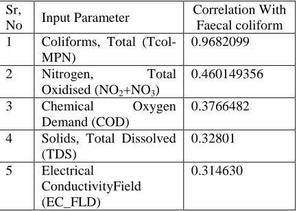
(FCol-MPN)(MPN/100ml) is used. Statistical and data driven techniques are used to find the most influential parameters and results are compared. between themselves and coliform (faecal) (output) and to what extent. (refer table no. 1) It was found that out of nineteen parameters seven are moderately (.50 to .31) correlated with Faecal coliform ( output). Only Total coliform is strongly correlated ( .968) with output. Table 2 shows the correlation of input variable with output variable in descending order.
Table 1: Correlation of input parameter with input and output
Variables TempEC_GENEC_FLDpH_GENPH_FLD DODO_SAT%TDSTcol-MPNP-TotNO2+NO3NH3-N NaFCol-MPNCOD CO3 Cl BOD3-27ALK-TOTAlk-Phen Temp 1.00 -0.05 -0.04 -0.16 -0.17 -0.08 0.32 -0.05 0.00 -0.18 -0.07 -0.12 -0.06 -0.05 -0.05 -0.12 -0.09 0.08 -0.17 -0.05
EC_GEN -0.05 1.00 0.99 0.08 0.02 -0.21 -0.21 0.98 0.34 0.21 0.30 0.13 0.70 0.31 0.52 0.35 0.69 0.49 0.79 0.38 EC_FLD -0.04 0.99 1.00 0.08 0.02 -0.24 -0.23 0.97 0.34 0.23 0.30 0.14 0.72 0.31 0.56 0.35 0.71 0.52 0.77 0.37 pH_GEN -0.16 0.08 0.08 1.00 0.45 0.08 0.03 0.07 -0.07 0.14 -0.09 -0.02 0.00 -0.02 -0.11 0.59 -0.01 -0.09 0.10 0.65
PH_FLD -0.17 0.02 0.02 0.45 1.00 -0.08 -0.14 0.03 -0.22 0.12 -0.03 0.02 0.02 -0.23 -0.19 0.26 -0.01 -0.12 -0.06 0.15 DO -0.08 -0.21 -0.24 0.08 -0.08 1.00 0.92 -0.16 0.16 0.06 0.07 -0.04 -0.16 0.20 -0.07 -0.08 -0.15 -0.18 -0.16 -0.02 DO_SAT% 0.32 -0.21 -0.23 0.03 -0.14 0.92 1.00 -0.16 0.15 -0.01 0.03 -0.08 -0.16 0.17 -0.08 -0.12 -0.17 -0.13 -0.21 -0.03 TDS -0.05 0.98 0.97 0.07 0.03 -0.16 -0.16 1.00 0.35 0.30 0.35 0.11 0.73 0.33 0.51 0.33 0.72 0.49 0.77 0.40 Tcol-MPN 0.00 0.34 0.34 -0.07 -0.22 0.16 0.15 0.35 1.00 0.08 0.52 -0.01 0.24 0.97 0.38 -0.01 0.24 0.19 0.16 0.18
P-Tot -0.18 0.21 0.23 0.14 0.12 0.06 -0.01 0.30 0.08 1.00 -0.13 0.18 0.28 0.11 0.39 0.12 0.29 0.43 0.24 0.19 NO2+NO3 -0.07 0.30 0.30 -0.09 -0.03 0.07 0.03 0.35 0.52 -0.13 1.00 -0.08 0.19 0.46 0.08 -0.04 0.18 -0.02 0.15 0.07 NH3-N -0.12 0.13 0.14 -0.02 0.02 -0.04 -0.08 0.11 -0.01 0.18 -0.08 1.00 0.01 -0.01 0.00 -0.03 0.02 0.02 0.04 0.03
Na -0.06 0.70 0.72 0.00 0.02 -0.16 -0.16 0.73 0.24 0.28 0.19 0.01 1.00 0.21 0.48 0.18 0.97 0.59 0.51 0.21 FCol-MPN -0.05 0.31 0.31 -0.02 -0.23 0.20 0.17 0.33 0.97 0.11 0.46 -0.01 0.21 1.00 0.38 0.00 0.22 0.20 0.14 0.20 COD -0.05 0.52 0.56 -0.11 -0.19 -0.07 -0.08 0.51 0.38 0.39 0.08 0.00 0.48 0.38 1.00 0.06 0.49 0.78 0.38 0.11 CO3 -0.12 0.35 0.35 0.59 0.26 -0.08 -0.12 0.33 -0.01 0.12 -0.04 -0.03 0.18 0.00 0.06 1.00 0.23 -0.06 0.41 0.57
Cl -0.09 0.69 0.71 -0.01 -0.01 -0.15 -0.17 0.72 0.24 0.29 0.18 0.02 0.97 0.22 0.49 0.23 1.00 0.55 0.50 0.20 BOD3-27 0.08 0.49 0.52 -0.09 -0.12 -0.18 -0.13 0.49 0.19 0.43 -0.02 0.02 0.59 0.20 0.78 -0.06 0.55 1.00 0.33 0.10 ALK-TOT -0.17 0.79 0.77 0.10 -0.06 -0.16 -0.21 0.77 0.16 0.24 0.15 0.04 0.51 0.14 0.38 0.41 0.50 0.33 1.00 0.44 Alk-Phen -0.05 0.38 0.37 0.65 0.15 -0.02 -0.03 0.40 0.18 0.19 0.07 0.03 0.21 0.20 0.11 0.57 0.20 0.10 0.44 1.00
To find the significant inputs, correlation of each parameter with output was found. Table 1 shows correlation of input parameters with each other and
correlation of input parameters with output parameter (faecal coliform).It was found that out of nineteen, seven parameters are moderately correlated with output i.e with faecal coliform. Table 2 shows the correlation of input parameters with output in descending order.
Table 2: Correlation of input parameters with output
Sr,
Table 2 shows that total coliform are highly correlated with faecal coliform.(correlation coefficient 0.968) as compared with total oxidized Nitrogen , chemical oxygen demand, total dissolved solids, and electrical conductivity.
The major disadvantage associated with using correlation analysis is that it is only able to detect linear dependence between two variables. Therefore such an analysis is unable to capture any non linear dependence that may exist between the input and output and may possibly result in the omission of important inputs that are related to the output in non linear fashion [8]
4.2 By use of principal component analysis(PCA)
Principal Component Analysis is a powerful pattern recognition technique that attempts to explain the variance of a large dataset of inter-correlated variables with a smaller set of independent variables (principal components) [13]. Many researchers have used the data processing and dimension reduction techniques with numerous application in engineering, biology, biomedical engineering and social science.[5,13,17]. It is also used to evaluate the relationship between chemical variables and to local and regional processes which influence quality of water.[14].
The purpose of using PCA is to reduce
84
difference in their scales but having equalimportance.[17] A correlation matrix was therefore used for the application of PCA.While applying PCA the number of components extracted is equal to the interpretation and were used to present the data. Three criteria Kaiser eigenvalue-one criterion, Cattell Scree test, and Cumulative percent of variance were used to find meaningful components.
i) Kaiser Method
The Kaiser (1960) method provides a handy rule of thumb that can be used to retain meaningful components. This rule suggests keeping only components with eigenvalues greater than 1. This method is also known as the eigenvalue-one criterion. The rationale for this criterion is straight forward. Each observed variable contributes one unit of variance to the total variance in the data set. Any component that displays an eigenvalue greater than 1 is accounts for a greater amount of variance than does any single variable. Such a component is therefore accounting for a meaningful amount of variance, and is worthy of being retained. On the other hand, a component with an eigenvalue of less than 1 accounts for less variance than does one variable. The purpose of principal component analysis is to reduce variables into a relatively smaller number of components; this cannot be effectively achieved if we retain components that account for less variance than do individual variables. For this reason, components with eigenvalues less than 1 are of little use and are not retained.
Table 3 provides the eigenvalues from the PCA
applied to our dataset. In the column
headed“Eigenvalue”, the eigenvalue for each
component is presented. Each row in the table presents information about one of the 20components: the row“1” provides information about the first component (PCA1) extracted, the row “2” provides information about the second component (PCA2) extracted, and so on . Eigenvalues are ranked from the highest to the lowest. It can be seen that the eigenvalue for component 1 is 6.504, while the eigenvalue for component 2 is 2.738 This means that the first component accounts for 6.504 units of total variance while the second component accounts for 2.738 units. The third component accounts for about 2.28 unit of variance
Table 3 shows that the first component has an eigenvalue substantially greater than 1. It therefore explains more variance than a single variable, in fact 6.504 times as much. The second component displays an eigenvalue of 2.738, and component third to seventh ranges from 2.280 to 1.019 which are
substantially greater than 1, whereas eighth
component displays an eigenvalue of 0.870 which is
clearly lower than 1.The application of the Kaiser
criterion leads to retain unambiguously the first seventh principal components.
Table 3: Eigenvalues
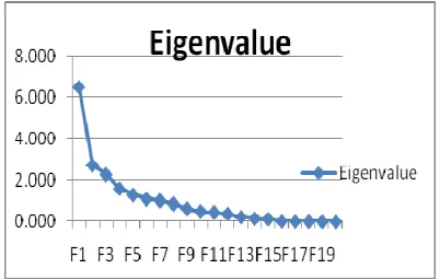
ii) Cattell Scree test
The scree test is another device for determining the appropriate number of components to retain. First, it graphs the eigenvalues against the component number. As eigenvalues are constrained to decrease monotonically from the first principal component to the last, the scree plot shows the decreasing rate at which variance is explained by additional principal components. To choose the number of meaningful components, we next look at the scree plot and stop at the point it begins to level off (Cattell, 1966; Horn, 1965). The components that appear before the “break” are assumed to be meaningful and are retained for interpretation; those appearing after the break are assumed to be unimportant and are not retained. Between the components before and after the
85
successive component is accounting for smaller andsmaller amounts of total variance. First two principal components account for about 57.66% of total variance.
Fig. 1:Eigen value
4.3 Cumulative percent of total variance
The percentage of variance accounted for by each component and the cumulative percent variance are presented in Table 5. From this Table it can be seen that the first component alone accounts for 32.518% of the total variance and the second component alone accounts for 13.690% of the total variance.and so on. Thus first 10 components when added the percentages together results in a sum of 92.784%. This means that the cumulative percent of variance accounted for by the first ten components is about 93%. This provides a reasonable summary of the data. Thus we can keep the first ten components and “throw away” the other components.
4.4 Interpretation of principal components
The correlation between each variable (20) and each principal component are given in Table 4
Table 4: Correlations between variables and factors:
F1 F2 F3 F4 F5 F6 F7 F8 F9 F10 F11 F12 F13 F14 F15 F16 F17 F18 F19 F20
Temp -0.11 0.23 -0.10 0.11 0.71 -0.28 0.27 0.48 -0.05 0.14 -0.06 0.05 -0.01 0.03 -0.07 -0.01 0.00 0.00 0.00 -0.01
EC_GEN 0.93 -0.06 -0.01 -0.11 0.14 0.17 0.12 0.02 -0.13 -0.08 -0.07 -0.06 0.10 -0.06 0.06 0.02 0.02 -0.03 0.06 0.00
EC_FLD 0.94 -0.06 -0.04 -0.09 0.12 0.13 0.11 0.04 -0.12 -0.08 -0.06 -0.02 0.11 -0.08 0.04 0.01 0.01 -0.07 -0.05 0.00
pH_GEN 0.12 -0.57 0.65 0.11 -0.04 -0.22 -0.06 0.10 0.09 -0.13 0.17 -0.01 0.29 0.06 -0.12 0.00 -0.01 0.01 0.00 0.00
PH_FLD -0.01 -0.56 0.23 0.02 -0.16 0.14 -0.41 0.51 -0.26 -0.13 -0.17 -0.13 -0.16 0.02 -0.01 -0.01 0.00 0.00 0.00 0.00
DO -0.21 0.44 0.61 0.45 0.04 0.37 -0.08 -0.16 -0.02 -0.10 0.00 -0.01 -0.02 0.00 0.03 0.00 0.00 0.00 0.00 -0.02
DO_SAT% -0.23 0.50 0.54 0.48 0.32 0.24 0.03 0.04 -0.04 -0.04 -0.01 0.01 -0.01 0.01 0.00 0.00 0.00 -0.01 0.00 0.02
TDS 0.94 -0.03 0.02 -0.06 0.12 0.19 0.07 0.03 -0.14 0.03 -0.02 -0.05 0.09 -0.09 0.08 -0.03 -0.03 0.09 -0.01 0.00
Tcol-MPN 0.45 0.65 0.35 -0.28 -0.24 -0.23 0.02 0.11 0.08 0.02 -0.16 -0.09 -0.03 0.02 -0.02 0.11 -0.02 0.02 0.00 0.00
P-Tot 0.38 -0.08 0.02 0.59 -0.44 -0.10 -0.01 0.05 -0.18 0.50 -0.05 0.07 0.06 -0.03 0.00 0.00 0.01 -0.01 0.00 0.00
NO2+NO3 0.31 0.40 0.24 -0.56 -0.04 0.21 -0.22 0.15 -0.21 0.12 0.32 0.31 -0.02 0.04 -0.02 -0.01 0.00 -0.01 0.00 0.00
NH3-N 0.09 -0.09 -0.08 0.09 -0.46 0.39 0.65 0.34 0.18 -0.11 0.05 0.09 -0.05 0.04 -0.03 0.00 0.00 0.00 0.00 0.00
Na 0.82 0.01 -0.18 0.13 0.13 0.16 -0.29 0.09 0.35 0.07 0.04 -0.04 -0.03 0.02 -0.04 0.01 0.10 0.02 0.00 0.00
FCol-MPN 0.43 0.63 0.39 -0.23 -0.27 -0.26 0.03 0.07 0.10 -0.01 -0.16 -0.12 0.03 0.05 0.02 -0.11 0.01 -0.01 0.00 0.00
COD 0.67 0.28 -0.20 0.31 -0.15 -0.31 -0.02 -0.11 -0.16 -0.30 -0.01 0.18 -0.10 -0.14 -0.17 -0.01 0.01 0.01 0.00 0.00
CO3 0.37 -0.56 0.47 -0.05 0.13 -0.13 0.06 -0.15 0.13 -0.01 -0.30 0.38 -0.08 0.05 0.09 0.00 0.01 0.01 0.00 0.00
Cl 0.81 0.01 -0.18 0.12 0.10 0.17 -0.28 0.05 0.39 0.07 0.00 0.02 -0.04 -0.01 -0.05 -0.01 -0.09 -0.03 0.01 0.00
BOD3-27 0.64 0.16 -0.36 0.43 -0.04 -0.29 -0.08 0.09 -0.08 -0.19 0.19 0.03 -0.01 0.21 0.18 0.01 -0.01 0.00 0.00 0.00
ALK-TOT 0.77 -0.20 0.04 -0.07 0.13 0.15 0.19 -0.36 -0.22 0.09 -0.04 -0.15 -0.10 0.22 -0.15 0.00 -0.01 0.00 0.00 0.00
Alk-Phen 0.45 -0.37 0.57 -0.01 0.07 -0.27 0.21 -0.03 0.08 0.08 0.33 -0.15 -0.23 -0.12 0.06 0.00 0.00 -0.01 0.00 0.00
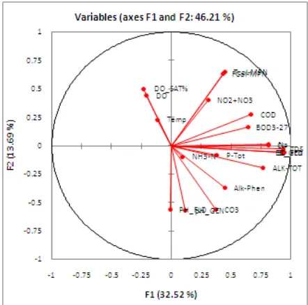
A coefficient greater than 0.4 in absolute value is considered as significant (see, Stevens (1986) for a discussion). We can interpret F1 as being highly positively correlated with variables EC-GEN, EC-FLD, TDS, TCol-MPN, Na, FCol-MPN,
COD, Cl, BOD,ALK-TOT, ALK-Phen,.so these
86
Fig. 2: Data set loading with two componentsThe principal component analysis allows us to reduce the dimensional representation of variable in the plane constructed from the first two components. Fig. 2 represents this graph for our dataset. For each variable we have plotted on the horizontal dimension its loading on component 1, on the vertical dimension its loading on component 2. The graph also presents a visual aspect of correlation patterns among variables. The cosine of the angle between two variables is interpreted in terms of correlation. Variables highly positively correlated with each another show a small angle, while those are negatively correlated are directed in opposite sense, i.e. they form a flat angle. From Fig. 2 we can see that the 20 variables hang together in three distinct groups. EC-GEN, EC-FLD, TDS, Na, Cl, form one group whereas FCol-MPN TCol-MPN,
NO2+NO3, form second group and DO, DO%,
temperature form third group. In a subspace of components, the quality of representation of a variable is assessed by the sum-of-squared component loadings across components. This is called the communality of the variable. It measures the proportion of the variance of a variable accounted for by the components. For example, in our example, the communality of the
variable temp is -0.1142+0.2322
+(-0.098)2+0.1062+0.7052+(-0.278)2+0.2742
=0.7376. This means that the first seven components explain about 74% of the variance of the variable temp.. This is quite substantial to enable us fully interpreting the variability in this variable as well as its relationship with the other variables. Communality can be used as a measure of goodness-of-fit of the projection. The
communalities of the 20 variables of our data are displayed in Table 5
As shown by this Table, the first seven components explain more than 74% of variance in each variable. This is enough to reveal the structure of correlation among the variable
Table5: Communality of 20 parameters
Table 6: Contribution of each variable
F1 F2 F3 F4 F5 F6 F7 F8 F9 F10 F11 F12 F13 F14 F15 F16 F17 F18 F19 F20 Temp 0.20 1.96 0.42 0.70 38.32 7.08 7.39 26.22 0.42 4.00 0.78 0.55 0.03 0.44 3.36 0.22 0.02 0.01 0.04 7.84 EC_GEN 13.36 0.12 0.01 0.72 1.49 2.49 1.35 0.03 2.74 1.17 0.95 0.86 4.69 2.50 2.63 1.22 1.35 5.66 56.64 0.00 EC_FLD 13.69 0.12 0.06 0.53 1.15 1.53 1.21 0.14 2.24 1.35 0.69 0.14 5.15 3.70 0.99 0.83 0.49 26.28 39.62 0.09 pH_GEN 0.21 11.83 18.73 0.72 0.14 4.52 0.40 1.21 1.26 3.38 6.03 0.01 37.30 2.50 11.10 0.08 0.21 0.33 0.02 0.03 PH_FLD 0.00 11.53 2.28 0.04 1.91 1.87 16.61 30.04 10.84 3.23 6.15 4.17 10.78 0.23 0.10 0.13 0.06 0.02 0.00 0.00 DO 0.66 7.09 16.38 12.81 0.11 12.54 0.70 3.08 0.07 1.84 0.01 0.01 0.19 0.01 0.69 0.06 0.00 0.00 0.00 43.75 DO_SAT% 0.83 9.21 12.98 14.50 7.78 5.30 0.10 0.19 0.25 0.26 0.01 0.04 0.06 0.04 0.00 0.01 0.00 0.24 0.02 48.19 TDS 13.59 0.02 0.02 0.24 1.20 3.18 0.46 0.14 2.88 0.20 0.08 0.56 3.41 5.45 4.24 2.84 4.17 54.98 2.29 0.07 Tcol-MPN 3.07 15.36 5.42 4.92 4.33 4.88 0.03 1.47 1.12 0.09 5.29 2.17 0.27 0.37 0.25 47.52 1.32 1.98 0.12 0.01 P-Tot 2.21 0.26 0.02 21.61 14.75 0.84 0.01 0.31 4.90 50.05 0.53 1.10 1.63 0.74 0.01 0.06 0.13 0.75 0.08 0.00 NO2+NO3 1.47 5.84 2.52 19.33 0.11 3.98 4.92 2.52 6.64 3.03 21.69 25.59 0.19 1.21 0.42 0.15 0.04 0.28 0.07 0.00 NH3-N 0.13 0.33 0.28 0.55 16.05 14.12 42.07 13.29 4.87 2.44 0.65 2.13 0.92 1.21 0.78 0.02 0.00 0.14 0.00 0.00 Na 10.25 0.00 1.48 1.06 1.27 2.38 8.29 1.04 19.56 0.84 0.41 0.40 0.38 0.27 1.48 0.33 47.49 2.81 0.25 0.00 FCol-MPN 2.84 14.71 6.58 3.22 5.71 5.97 0.08 0.58 1.64 0.01 5.55 3.55 0.28 1.66 0.44 44.82 1.01 1.31 0.04 0.00 COD 6.88 2.80 1.75 6.15 1.63 8.71 0.04 1.28 4.15 17.36 0.01 8.69 4.22 12.66 22.42 0.43 0.17 0.51 0.14 0.00 CO3 2.10 11.42 9.61 0.14 1.33 1.47 0.41 2.44 2.54 0.01 19.79 37.78 2.63 1.87 5.90 0.02 0.33 0.18 0.01 0.01 Cl 10.16 0.00 1.35 0.94 0.78 2.61 7.48 0.32 24.31 0.97 0.00 0.16 0.78 0.09 2.17 0.79 42.54 3.96 0.58 0.00 BOD3-27 6.27 0.95 5.72 11.51 0.14 7.57 0.57 0.86 1.00 6.82 8.04 0.19 0.02 26.06 23.32 0.38 0.54 0.01 0.02 0.00 ALK-TOT 9.01 1.43 0.06 0.30 1.37 2.08 3.56 14.76 7.56 1.66 0.27 5.83 4.67 30.19 16.94 0.08 0.14 0.03 0.06 0.00 Alk-Phen 3.05 5.01 14.32 0.01 0.43 6.88 4.30 0.10 1.03 1.27 23.08 6.05 22.38 8.80 2.76 0.00 0.01 0.52 0.00 0.00
87
Table 7:Significant variables by PCA
4.5 Forecasting by use Genetic Programming
For the variable sets shown in table 7 GP runs
were taken with the function set +,_,*,/.x2 and
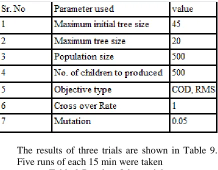
following parameters were used for the runs. Table 8: Parameters used for GP runs.
The results of three trials are shown in Table 9. Five runs of each 15 min were taken
Table 9:Results of three trials
5 Input selection by Genetic Programming
An advantage of using Genetic Programming for the modeling process is its ability to produce models that are in the form of an interpretable equation. Since GP evolved equations relating input and output variables
might shed physical insight into the ecological processes involved, they are used to identify the significant variables.[8].Table 10 shows the GPkernel parameters used for all GP runs for the selection of significant input.
The maximum initial tree size was restricted to 45 and maximum tree size was selected to be 20 because GP has a tendency to evolve uncontrollably large trees if the tree size is not limited [11.] Maximum tree size 20 has another advantage. Restricting to this size evolves simple expressions that are easy to interpret and contains only four to eight variables which are most significant and comfortable to handle [8,11].The values of population size, no. of children to produced, objective type, cross over Rate, mutation were fixed by referring earlier researchers work [1, 8, 9, 11] For GP runs four different simple mathematical operators [1, 11] are used as function sets. (Refer Table no 11). Small and simple function sets are used because GP is very creative at taking simple functions and creating what it need by combing them [7].( Banzhaf w, Nordin p, Genetic programming an Introduction is a book)A simple function set also leads to evolution of simple GP models which are easy to interpret[7]. Thus 40 GP equations were evolved for 30 days ahead prediction. As GP has ability to find the significant input variable, it is expected that GP evolves equations which contains most significant variables out of the total 19 input variables. It is measured by considering no of times the variable is selected in equation [1, 8]. Table12 shows the summary of no. of times the input variables in all 40 equations.
Table 10: Parameters used for GP runs.
88
Table 12: Summary of no. of times the input variablesin all equations
The significant variables are highlighted. These variables are those whose numbers of terms are more than 2% of the total number of terms in GP equations [8,6]
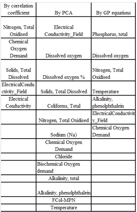
Table 13 : Significant variables by correlation coefficient and by PCA and BY GP equations
From the above three methods it was found that the most significant input parameter selection can be done by Genetic Programming which gives equally competent results as compared with statistical analysis with comparatively less time consumption for
the process. Input parameters selected for prediction
of water quality are Coliforms, Total (Tcol-MPN), Phosphorus, total, Dissolved oxygen, Nitrogen, Total
Oxidised (NO2+NO3 ),Temperature, Alkalinity,
phenolphthalein, Electrical Conductivity Field
(EC_FLD), Chemical Oxygen Demand (COD), faecal coliform. The values of these parameters at time t to t-6 may influence the prediction process [8,11].With these nine parameters GP equations were evolved to develop relationship between faecal coliform at time t and nine input variables with a time lag of t to t-6 . Thus for each of the nine input variables, we have 7 time lagged variables, making total (9 x 7) 63 input variables.
89
Table 14:Summery of Number of Times InputVariables in 60 Equations
Total terms in all runs are 516. Highlighted parameters are indicative of the contribution more than 2%. The most significant parameters to predict faecal coliform 30 days ahead in advance are presented in table 15
Table 15: Significant Parameters By GP
5.1 Genetic Programming Modeling
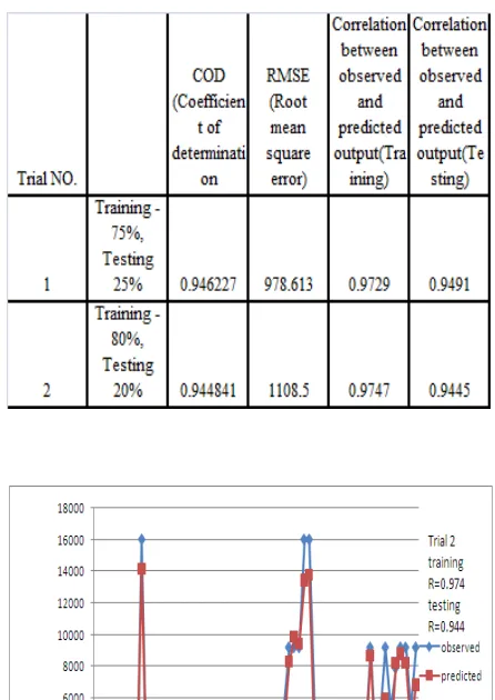
The standard GP model was evolved for the prediction of faecal coliform 30 days in advance . The input variables selected are taken from the significant input selection model which was previously described in the above section. Refer table 8. The parameters of GP runs are same as shown in table 1. Runs were
taken by using training and testing data 75% and 25 % .The results are tabulated in the Table 16
Table 16: Results of GP
Fig. 3: Graph of Observed and Predicted output The results are shown in Fig. 3
Model developed with the significant inputs to predict faecal coliform at chaskaman reservoir is presented in fig 3. The perditions are satisfactory with reasonably good peak value predictions.
6. Results and Discussion:
Monthly Water quality data from July 2000 to
October 2011 collected by Government of
90
significant input parameters due to its non linearrelationship. One of the data mining technique Principal Component Analysis results are presented in table no. 10 which gives 15 significant input parameters. Genetic Programming was also used to find the significant input parameters. For 20 variables runs are taken and 40 equations are evolved and occurrence of each variable in 40 equations is found. Total terms in GP models are 263. The significant variables are those whose numbers of terms are more than 2% of the total number of terms in GP equations. By this method 8 parameters are found significant presented in table no.5.
By using these 8 parameters again GP runs are taken for time lag t to t-6. From 63 input parameters 11 parameters are found significant presented in table no. 15. For these 11 parameters again GP runs are taken and that is for 2 trials. Results are presented in table no.16. and compared with the results of parameters selected from PCA. Result shows that RMSE by GP is 978.613which is better than that by PCA parameter which is 2022.13. Results of correlation coefficient
between observed and predicted output and
coefficient of determination by both methods are comparable.
7. Acknowledgement:
The Authors wish to thank Government of Maharashtra, Water Resource Department, Hydrology Project (surface water), Hydrological Data User Group for providing water quality data for the study.
References:
[1]. D M Hamby,1994 “Review of techniques for
parameter sensitivity analysis of Environmental
models”, Environmental Monitoring and
assessment, Sept. 1994-Springer, Volume32,
Issue2, pp135-154
[2]. Hopke P K.1985 Receptor modeling in
environmental chemistry. USA: Wiley; 1985.
[3]. Igor Shiklomanov's chapter "World fresh water
resources" in Peter H. Gleick (editor), 1993, Water in Crisis: A Guide to the World's Fresh Water Resources (Oxford University Press, New York).]. ga.water.usgs.gov/edu/waterdistribution
[4]. Koza John, “ Genetically breeding populations
of computer programs to solve problems in Artificial Intelligence”.1992
[5]. Nazire MazlumAdem ozer, Suleyman
Mazlum,1999 “ Interpretation of water quality data by Principal component Analysis”Tr.J.of
Engineering and Environmental science, 23 ,
19-26
[6]. Nitin muttil , J.H.W. Lec and A.W.
Jayawardena.2004“Real time prediction of
coastal algal blooms using genetic
programming”, 6th international Conference on
hydro informatics
[7]. Nitin Muttil and Kwok-wing Chau,2006“Neural
Network and Genetic programming for modeling costal algal blooms” International Journal of
Environment and Pollution, Vol. 28 No. 3-4,
pp223-238
[8]. NitinMuttil,Kwok-wing Chau,2007“Machine
learning paradigms for selecting ecologically
significant input variable”,Engineering
Applications of Artificial Intelligence, Vol. 20
No. 6,pp.735-744
[12]. V. Simeonova,, J.A. Stratisb , C. Samarac et
al.,2003 “Assessment of the surface water
quality in Northern Greece”, Water
Research 37 (2003) 4119–4124
[13]. Varun Gupta, Rmveer Singh et al 2011, “An
Introduction of Principal omponent Analysis and
its importance in biomedical signal
processing”,nternational conference on life
science and technology IPCBEE vol 3 ,
[14]. Vikram Bhardwaj et.al.,2010 “Water quality
of the chhoti Gandak Riverusing principal component analysis, Ganga Plain, India”, J.
Earth Sci 119, No.1 Feb 2010. Pp 117-127
[15]. Why Study Lakes? An Overview of USGS