Representation of 3D and 4D Objects Based on an Associated Curved Space and a General Coordinate Transformation Invariant Description

Volume 2007, Article ID 42505,10pages doi:10.1155/2007/42505

Research Article

Representation of 3D and 4D Objects Based on

an Associated Curved Space and a General Coordinate

Transformation Invariant Description

Eric Paquet

Visual Information Technology Group, National Research Council, M-50 Montreal Road, Ottawa, ON, Canada K1A 0R6

Received 25 January 2006; Revised 24 July 2006; Accepted 26 August 2006

Recommended by Petros Daras

This paper presents a new theoretical approach for the description of multidimensional objects for which 3D and 4D are particular cases. The approach is based on a curved space which is associated to each object. This curved space is characterised by Riemannian tensors from which invariant quantities are defined. A descriptor or index is constructed from those invariants for which statistical and abstract graph representations are associated. The obtained representations are invariant under general coordinate transfor-mations. The statistical representation allows a compact description of the object while the abstract graph allows describing the relations in between the parts as well as the structure.

Copyright © 2007 Eric Paquet. This is an open access article distributed under the Creative Commons Attribution License, which permits unrestricted use, distribution, and reproduction in any medium, provided the original work is properly cited.

1. INTRODUCTION

Content-based description plays a prominent role in index-ing and retrieval [1–4]. It is therefore important to develop invariant representations for 3D objects. An excellent review about indexing and retrieval of 3D objects can be found in [1–3]. As can be seen from this review, most of the proposed techniques are invariant under a very limited class of trans-formations, for example, translations, scaling, and rotations. Relatively less attention has been devoted to the development of representations that are invariant undergeneral coordinate transformations. In addition, most approaches are limited to 3D objects understood in the sense of 2-D surfaces embed-ded in 3D space (e.g., a VRML object) and cannot be applied to volumetric objects, like those generated by tomography. Such multidimensional objects are characterised by the fact that each point in 3D space (volumetric space) is associated with a set of attributes. For instance, in the case of tomog-raphy, the set is generally limited to one attribute, the den-sity, and the map is called a 4D object. This paper presents a new approach for invariant description of multidimensional objects under general coordinate transformations leading to a new type of representation based on the Ricci tensor and scalar. This novel approach transposes certain results of gen-eral relativity [5–7] and Riemannian geometry [5] into the framework of computer vision.

The paper is organised as follows. After some considera-tions on content-based indexing and retrieval, we review the most important results of tensor analysis which are necessary to understand our approach. Then, a tensor is associated to each object and the fundamental equations are derived from a variational principle. This tensor describes the attributes of the object and becomes the source for an associated curved space. The geometry of this associated curved space is de-scribed by a quadric form or a metric, a Ricci tensor and a Ricci scalar from which invariant quantities are derived. Fi-nally, two representations are adopted for the invariants. The first one is a statistical representation based on a novel his-togram and the second representation is a topological one based on an abstract graph. These representations are invari-ant under general coordinate transformations.

2. CONTENT-BASED DESCRIPTION OF 3D AND 4D OBJECTS

Figure1: Four views of a tomographic image of the brain. The in-tensity is related to the density. Each slice corresponds to a certain elevation in the brain.

multidimensional content is problematic due to the high number of dimensions involved, their heterogeneity (space, time, speed, density, field intensity, etc.), and the fact that the standard mathematical framework has proven itself to be not suitable to derive form invariant equations under arbi-trary coordinate transformations [5–7]. Form invariance is important in order to construct a description that is invari-ant under arbitrary coordinate transformations. This means that, no matter how the initial object is transformed (as de-fined inSection 3), the associated description is always the same. A new approach is presented to this paper, based on tensor analysis, in which a Riemannian space or curved space (as opposed to standard flat Euclidian space) is associated to an object. This space is described by tensorial equations which are form invariant under arbitrary coordinate trans-formations. A set of invariant quantities are extracted from this space and a representation is constructed from the set of invariants. Two types of representation are considered: Rie-mannian histograms and abstract graphs.

3. AN OVERVIEW OF TENSOR ANALYSIS

In this section, an overview of tensor algebra is presented. Derivations and more details can be found in [5–8]. This section is a prerequisite for what follows. Unless stated oth-erwise, all Greek indices and all summations are to be taken from 1 toN. Furthermore, if an index is not involved in a summation, it is immaterial and can be replaced by any other index.

The use of tensorial analysis is justified by the fact that tensorial equations do not change their form under arbitrary

coordinate transformations. We assume that the space has an arbitrary number of dimensions, which means that the equa-tions that we will derive could be applied to both 3D and 4D objects. A point in space is given by

x=xμ_{. (1)}

For instance, in 3D

x= ⎛ ⎜ ⎝

x1 x2 x3

⎞ ⎟ ⎠=

⎛ ⎜ ⎝

x y z

⎞ ⎟

⎠. (2)

We assume that it is possible to associate to the space a metric

gμν(x), which is defined by the quadratic form

ds2≡ μνgμν

(x)dxμdxν. (3)

In other words, we assume that we can define an invari-ant distancelocally. This is an important distinction in be-tween standard Euclidian geometry and Riemannian geom-etry: distance is aglobalinvariant (for orthogonal transfor-mations) for the former and a local invariant for the lat-ter (under general coordinate transformations). Indeed, be-cause of the space curvature, it is not possible to define a global metric. It should be noticed thatds, the infinitesimal length of arc, is an invariant and has the same value irre-spectively of the coordinate system. Note that this metric de-fines the inner product between two tensors for the curved space.

The covariant and a contravariant vector are defined, re-spectively, as

Aμ(x)=

ν

∂xν(x)

∂xμ Aν(x), B

μ_(x)= ν

∂xμ_(x)

∂xν Bν(x),

(4)

where

xμ=xμ(x), xν=xν(x) (5)

Of course, if the axes of the reference frame are normal, the parallel and the normal projections are identical.

In general, p contravariant and qcovariant tensors are defined as

Tμ1···μp

ν_1···νq(x)

=

μ1···μp,ν1···νq

∂xμ1_(x)

∂xμ1 · · ·

×∂xμp(x)

∂xμp

∂xν1_(x)

∂xν1 · · ·

∂xνq_(x)

∂xνq T

μ1···μp

ν1···νq(x).

(6)

At this point we should make a few remarks about the gen-eral coordinate transformations. It can be shown [5–8] that tensorial calculus is valid if and only if the general coordi-nate transformations are continuously differentiable which means that the transformations are continuous and smooth at any order. Furthermore, the mapping between the origi-nal coordinates and the transformed coordinates should be biunivoque which means that to each point corresponds one and only one transformed point, and vice versa. These con-straints ensure that not only the tensorial equations are valid, but that an object cannot be transformed arbitrarily into an-other object. This is a fundamental requirement for searching and retrieval. Any transformation that satisfied the above-mentioned requirements is compatible with our approach.

We will admit the following results without demonstra-tion [5–8]. The metric is a symmetric tensorgμν(x)=gνμ(x). If a tensor is identically zero in a coordinate system, it is equal to zero in any other coordinate system. The product of a ten-sor by a tenten-sor is a tenten-sor and so is the sum. The symmetry and antisymmetry properties of a tensor are conserved under general coordinate transformations and so are the symmetry properties of the corresponding object. In addition, the most important property can be stated as follow: a tensorial equa-tion does not change form under general coordinate trans-formations. Such a feature is highly desirable if one seeks to define quantities that are coordinate transformations invari-ant, that is, quantities that can describe an object irrespec-tively of its state of transformation. Furthermore, the follow-ing relations will be of use:

ρ

∂xμ_(x)

∂xρ

∂xρ_(x)

∂xν =δ

μ

ν, (7)

gμν(x)=

ρ

∂xρ_(x)

∂xμ

∂xρ_(x)

∂xν , (8)

ρ

gμρ_(x)g

νρ(x)=δμν. (9)

The metric has an additional important property; it can transform covariant indices into contravariant indices and vice versa as illustrated by the following equation:

Aμν(x)=

αβ

gμα(x)gνβ(x)Aαβ(x). (10)

The derivative of a tensor is not a tensor. Indeed, if one cal-culates the derivative of a covariant vector, one obtains

∂Aμ(x)

∂xν =

ρσ

∂xρ_(x)

∂xμ

∂xσ_(x)

∂xν

∂Aρ(x)

∂xσ +

ρ

Aρ(x)∂

2_xρ_(x)

∂xμ_∂xν. (11)

The first term of the right member has the correct form as defined by (4), that is, it is transformed as a tensor, but the second term is incompatible with the definition of a tensor (the transformation involves the second-order derivative of

xρ_{(x)). Nevertheless, one can define a covariant derivative,} which is form invariant under general coordinate transfor-mations

∇νAμ(x)≡

∂Aμ(x)

∂xν −

σ

Γσ

μν(x)Aσ(x), (12)

whereΓσ

μνis named the affine connection and is related to the metric by the following relation:

Γσ μν(x)=

ρ

1 2g

σρ_(x)

∂gμρ(x)

∂xν + ∂gρν(x)

∂xμ −

∂gμν(x)

∂xρ

. (13)

It should be noticed that the affine connection is not a ten-sor. Irrespectively on the mathematics involved, the covari-ant derivative is a simple concept. The derivative in Euclid-ian space is related to the concept of slope or in other words the difference in between two points at two distinct posi-tions. Such an operation is not problematical in standard Eu-clidian geometry since the space is flat, homogeneous, and isotropic. In our case, the space is not flat but curved and one cannot compare two points at two different locations be-cause they live so to say in two different spaces. What can be done though is to transport one of the vector “parallel” to itself to the other location and then to compare them on thesamelocation. This is what is expressed by (12) and the affine connection is responsible for such a parallel trans-portation.

Riemannian spaces are not conservative: if a vector is moved along a close path, the resulting vector does not co-incide in general with the original vector. That means again that it is not possible to compare two tensors at two distinct positions. One can easily convince oneself of that. For exam-ple, it suffices to move a vector from the North Pole to the equator along a meridian, then once more along the equa-tor, and finally back to the North Pole along a meridian: the initial and the final directions of the vector are different al-though the norm remains the same. Such a phenomenon happens because the Earth surface is a 2D curved surface: a sphere.

variation is proportional to the curvature tensor

ΔAμ(x)= −

C

νσ Γσ

μν(x)Aσ(x)dxν

=1 2

νστ

Rνμστ(x)Aν(x)dxσ∧dxτ,

(14)

where∧represents the external product and where the Rie-mannian curvature tensorRνμστ(x) is defined as

Rνμστ(x)≡

∂Γνμτ(x)

∂xσ −

∂Γνμσ(x)

∂xτ

+

ρ Γν

ρσ(x)Γ ρ

μτ(x)−Γνρτ(x)Γ ρ μσ(x).

(15)

From the inner product between the metric and the Rieman-nian curvature tensor, one can define the Ricci tensorRνσ(x) and the Ricci scalarR(x) which are, respectively, given by

Rνσ(x)= μτρ

gμρ_(x)g

μτ(x)Rτ_νρσ(x), (16)

R(x)= νσ

gνσ(x)Rνσ(x). (17)

The Ricci tensor is symmetric. The Ricci tensor and scalar satisfy many identities among which are the Bianchi identi-ties which are more or less a conservation identity:

α

∇α

Rσα_(x)−1 2g

σα_R(x)

=0. (18)

The Riemann tensor and the Ricci tensor and scalar charac-terise the curvature of the space at a given point. The Rie-mann and the Ricci tensor are not invariant under general coordinate transformations: they transform as tensors. How-ever, the Ricci scalar is an invariant: its value is the same irrespectively of the general coordinate transformation ap-plied. Such a feature is common to all scalars in a Riemannian space. At this stage, it is important to realise that the curva-ture is not bonded to a particular coordinate system but to the physical point itself. For instance, even if the Ricci scalar is an invariant, the coordinates of the point to which it is at-tached change under a GCT. InSection 5, we will see how we can represent invariant quantities independently of their coordinates.

There is a relation in between the Ricci scalar and the standard intrinsic Gaussian curvatures. One can demon-strate that in 2-D, the Ricci scalar and the intrinsic Gaussian curvatures are related by the relation

(2)_R(x)∝κ

1(x)κ2(x), (19)

whereκ1(x) andκ2(x) are the intrinsic Gaussian curvatures.

Such a relation does not exist in 3D or in higher dimensions. From that point of view, the Ricci scalar can be considered to a generalisation of the intrinsic curvatures to three dimen-sions and more.

4. ASSOCIATION OF A CURVED SPACE WITH AN OBJECT

In this section, a Riemannian curved space is associated with an object. A set of equations that are form invariant un-der general coordinate transformations are un-derived. In or-der to construct those equations, a tensor is associated with the object. Such an association can be realised, for instance, through the density of a tomographic image. This tensor acts as a source term in a field equation from which the geometry of the associated curved space is calculated.

The formulation of form invariant equations under gen-eral coordinate transformations is a complex task. It would be much easier if one could associate and define an invariant scalar functional from which the equations could be derived. Such an approach has been developed: the scalar functional is the Lagrangian and the equations are derived from a vari-ational principle or least action principle. For our purpose, the Lagrangian is a scalar functional related to the “energy of the system.” The energy could be related to the density of a tomographic image, the 3D shape deformation (like a deformable mesh), or some topological characteristics (like the number of holes in a certain neighbourhood). The reader who is not familiar with Lagrangians and variational princi-ples is referred to [5,8] for more details. Once the Lagrangian is defined, one can derive the corresponding equations by finding the extremum for the action associated with the La-grangian. We formulate the Lagrangian in such a way that it incorporates all our requirements about the curved space we want to associate with the object as well as all our knowledge (from an indexing and retrieval point of view) about the ob-ject itself.

In a Riemannian space, the actionS[5–7] is defined as

S≡

dNx

−detgμν(x)Lgμν(x), (20)

whereLis the Lagrangian (strictly speaking the Lagrangian density) and det(gμν(x)) the determinant of the metric (the metric is a matrix). One should notice that the action is also a scalar and consequently invariant under a GCT. The extra factor−det(gμν(x)) is related to the Jacobian of the trans-formation and ensures that the result of the integration does not depend on a particular choice of the coordinate system; in other words, the infinitesimal volume element (or hyper-volume) does not depend on the reference frame employed.

The principle of least action [5–8] states that if the action is extremal, the Lagrangian necessarily satisfies the Euler-Lagrange equations, which can be written in our specific case as

ρ

∂ ∂xρ

δ−detgμν(x)

Lgμν(x)

δ∂gμν(x)∂xρ

−δ

−detgμν(x)Lgμν(x)

δgμν(x) =0,

where δh[f(x)]/δ f(x) stands for the functional derivative (the derivative is calculated with respect to a function).

We are now in position to set our hypothesis and de-rive the corresponding equations. Let us assume that our Lagrangian can be split into two Lagrangians. The first La-grangianL[gμν(x)] depends solely on the metric and char-acterises the Riemannian space per se (the space we want to associate with our object) while the second Lagrangian

˘

L[gμν(x),Φ(x)] depends on the metric and some other ten-sorsΦthat characterise the object under consideration (e.g., the density in a volumetric image). It is very important to understand this point, the space associated with an object is not static but dynamics and its configuration depends on the energy content of the associated object. An analogy, although imperfect, is the association of a magnetic field to a current. As the current is the source of the magnetic field, the object is the source of the associated curved Riemannian space.

With these hypotheses in mind, the action can be written as

S=

dNx

−detgμν(x) Lgμν(x)+ ˘Lgμν(x),Φ(x). (22)

Let us write the Lagrangian for the associated curved space. We have seen earlier that a curved space can be characterised by a set of curvatures: the simplest one being the Ricci scalar. Consequently, one of the simplest Lagrangian that can be constructed from the Riemannian curvatures is the one con-structed from the Ricci scalar:

Lgμν(x)=κ−1R(x)=κ−1

μν

gμν(x)Rμν(x), (23)

where κis an arbitrary constant. Of course this is not the only possibility. One could take, for instance, the tensorial product of a covariant and contravariant Ricci tensor but that would lead to unnecessarily complicated equations. For our purpose, we will be satisfied with the simplest form possi-ble. If one substitutes (23) into (22) and optimised the action with (21), one obtains

δ S=0=⇒Rμν(x)− 1

2gμν(x)R(x)−κT˘μν(x)=0, (24)

where ˘Tμν, the source tensor, is associated with the object and is defined as

˘

Tμν(x)≡

δ−detgμν(x) _˘

Lgμν(x),Φ(x)

δgμν(x) . (25)

Because of (18) and (24), the source tensor satisfies the Bianchi identities and is symmetric. In other words, only those source tensors for which the covariant divergence is zero are acceptable. Consequently, when defining the source tensor, one has to be very careful in order to verify that the covariant divergence of (25) is effectively zero.

Next, one can demonstrate that the source tensor is re-lated to the density, the momentum, and the flux of momen-tum. For instance, for a static volumetric image one can

de-fine the source tensor as

˘

T00(x)=ρ(x) (26)

and zero otherwise, that is, the tensor is simply related to the density. In the general case, the source tensor is more com-plicated. More details can be found in [5–8] but the general approach is well known. One defines a Lagrangian that char-acterised the energy content of the object under considera-tion. Such a characterisation might be either physical (e.g., real physical density), topological, or formal. Then the source tensor is calculated from (25).

Finally, if one substitutes the value of the source tensor in (24), one obtains

Rμν(x)−1₂gμν(x)R(x)=κT˘μν(x) (27)

which is a set of ten (because of the symmetry properties of the tensors) form invariant nonlinear equations describing the relations in between the source tensor associated with the object and the curvatures of the corresponding Riemannian space. That is the relations we were looking for; we have as-sociated a curved space to the object.

In addition, it can be demonstrated [5–8] that the map-ping in between the source tensor (i.e., the object) and the Riemannian space is unique and consequently not ambigu-ous. This result is valid as long as the general coordinate transformations and the source tensor are continuously dif-ferentiable. That does not mean that transformations cannot vary rapidly, it only means that there should be no disconti-nuities (in the mathematical senses) in the transformations.

The solution of (27) is a highly nontrivial task. Never-theless, a numerical solution can be obtained by foliating the space; see, for instance, [9].

5. DEFINITION OF INVARIANT REPRESENTATIONS FROM A STATISTICAL REPRESENTATION AND FROM AN ABSTRACT GRAPH

Up to this point, we have associated a Riemann space to an object and we have characterised the curvature of this space by calculating the Ricci tensor and scalar distributions. Now, in order to obtain an invariant description, we must con-struct some invariant quantities from the Ricci curvatures. If one applies a coordinate transformation to the Ricci scalar, one obtains with the help of (7) and (17)

R=

μν

gμν_R

μν=R. (28)

Equation (28) shows that the Ricci scalar is invariant under arbitrary coordinate transformations and as a result we de-fine our first ensemble of invariant quantities1(x) as the

ensemble

1(x)| 1(x)≡R2(x)

If one computes the tensorial product of a covariant and a contravariant Ricci tensor, one obtains

μνR

μνRμν=

μνρσ

∂xμ

∂xρ

∂xν ∂xσ

Rμν

∂xρ

∂xμ

∂xσ

∂xν

Rμν

=

μνRμνR

μν (30)

which is again invariant under arbitrary coordinate transfor-mations. Consequently, we define our second ensemble of in-variant quantities2(x) as

2(x)| 2(x)≡

μνRμν

(x)Rμν_(x)

. (31)

As a result, an invariant statistical representation of the object can be constructed. The ensembles defined by (29) and (31) are described by two histograms. The first histogram charac-terises the distribution of the Ricci scalars while the second histogram characterised the distribution of the inner prod-ucts of the Ricci tensors. More precisely, the histograms are defined as

hk(i)≡

{x|[(iΔk−Δk/2)≤k(x)<(iΔk+Δk/2)]}

k(x), (32)

whereΔkis the width of each bin for histogramk.In other words, the histograms provide a statistical distribution for the invariants: they do not depend on the location of the in-variants on the object but only on their statistical distribu-tion. Such a distribution is invariant under a CGT and char-acterises the object.

For retrieval purpose, these histograms can be consid-ered as feature vectors and compared with standard tech-niques such as those described in [1,2]. For instance, com-parison can be performed with a metric (distance), a corre-lation technique, a neural network, or with a Bayesian ap-proach. Besides, whatever the method employed is, it is im-portant that a certain degree of cross-correlation (bins with different indexes) be present in the comparison algorithm because the invariants, as defined by (29) and (32), may pos-sibly present a certain bin index tolerance due to noise and inadequate sampling which means that bins could be shifted and the corresponding histograms distorted. For the metric approach, such a requirement can be implemented with a quadratic form.

An abstract graph representation is also possible. For such a graph, each point for which invariants are calculated is mapped to a node. Each node is related to the pair of in-variants calculated at the corresponding point and not to the coordinates of the points, which are in any case arbitrary. The only relations that are invariant, irrespectively of the GCT ap-plied to the object, are the adjacency relations in between the points. Such topological relations remain always the same, because the general coordinate transformations are contin-uously differentiable by hypothesis. The graph is then con-structed in such a way that adjacent nodes (i.e., points) are connected by lines or links. The link indicates only a con-nection in between two nodes; the length of the link has no

meaning per se, since the representation has to be invariant under a GCT. Such a graph is invariant under a GCT. The abstract graph obtained can be compared to another graph using standard techniques [1,2].

The histogram representation is much more compact and is adapted to very large databases. The compactness is obtained at the price of loosing the adjacency relations. The abstract graph approach preserves those relations, but the size of the graph limits its applicability to small subset of data for which a detailed representation might be needed.

6. PRACTICAL CONSIDERATIONS

The proposed method may be applied to a wide class of 3D objects. Nevertheless, there are some restrictions that should be taken into account; for instance, the objects under consid-eration should be Riemannian manifolds. In essence, a man-ifold is a surface (or a volume) that can be defined by a set of overlapping patches. The surface, included in the overlap-ping regions, should be continuously differentiable. Such a case is approximated, for instance, by the NURBS or nonuni-form rationalβ-splines which are widely utilise in computer graphics. The approximation comes from the fact that, in the NURBS representation, the overlapping regions are diff eren-tiable only up to a certain order. In addition to be a manifold, the surface should be Riemannian. That means that the sur-face should not present any torsion or, in other words, should not be twisted. For instance, if one cuts a circular band, twists the two extremities, and assembles them back together, one obtains a surface with torsion which cannot be described by the present approach. Otherwise, there are no restrictions and the considered surface can present holes, missing poly-gons, or other types of degeneracy.

For the vast majority of cases of interest, (27) must be solved numerically. As pointed out in [9], this is a difficult task in the sense that (27) is a set of 10 nonlinear differential equations. It has been shown [9] that such a set of equations can be numerically unstable if the numerical algorithm is not carefully designed: for instance, some constrains, like the Bianchi identities, that is, (18), must be enforced through-out the calculation. That means that for any practical appli-cation the calculation of the invariant representation must be performed offline. On the other hand, the retrieval op-eration can be performed in real time since the later involves only the comparison of histograms or graphs for which many real-time comparison approaches exist [1].

that the associated rotation matrix is a function of the coor-dinates on the object. Let us consider a GCT as defined by (4). Such an equation may be expressed in a matrix form as follows:

⎡ ⎢ ⎣

A0(x) A2(x) A3(x)

⎤ ⎥ ⎦= ⎡ ⎢ ⎢ ⎢ ⎢ ⎢ ⎢ ⎢ ⎢ ⎣

∂x0(x) ∂x0

∂x1(x) ∂x0

∂x2(x) ∂x0 ∂x0(x)

∂x1

∂x1(x) ∂x1

∂x2(x) ∂x1 ∂x0(x)

∂x2

∂x1(x) ∂x2

∂x2(x) ∂x2

⎤ ⎥ ⎥ ⎥ ⎥ ⎥ ⎥ ⎥ ⎥ ⎦ ⎡ ⎢ ⎣

A0(x) A1(x) A2(x)

⎤ ⎥ ⎦. (33)

The transformation matrix, which in fact is a matrix func-tional, is invertible by construction since the matrix elements are continuously differentiable. This transformation is ex-tremely general in the sense that the invariant representation does not depend on the form of this matrix. As a matter of fact, this matrix belongs to the group (in the mathematical sense) GL(3) of invertible matrices. We can consider a sub-group of GL(3): for instance, all the matrices for which the inverse is equal to the transpose of the transformation ma-trix. Such a matrix is the rotation matrix, that is, the group

O(3) of orthogonal matrices. Consequently, we have demon-strated that our approach is not only invariant for local rota-tions but also for much more general transformarota-tions. Con-sequently, our approach is a generalisation of global rotation invariance to local rotation invariance; in other words to lo-cal deformations.

7. EXPERIMENTAL RESULTS

In this section, we present experimental results. Our objec-tive is to better understand invariants (29) and (31). Firstly, we prove that they are invariant under a general coordinate transformation by explicitly applying such a transformation. Then, we evaluate invariant (29) for particular symmetries of the source tensor. We do not present any evaluation of in-variants (31) because they are too cumbersome. These calcu-lations are performed for both 3D and 4D objects, in order to better understand the differences in between the two. All the results that follow have been obtained symbolically with the Wolfram Research Mathematica software. All the calcu-lations were performed without any approximation. Conse-quently, the obtained results are exact. They can be utilised either as analytical expressions or as formulas in numerical evaluations. The results are presented with the Mathematica notation [10].

Firstly, we want to prove that our invariants are indeed invariant under a general coordinate transformation or GCT. For this purpose, we apply a GCT to invariant (29) and (31). The calculation is completely general and is performed for both 3D and 4D objects.

First, let us consider the case of three-dimensional ob-jects. If we make the summation explicit, invariant (29) could be written as

R11

R11_{+ 2R} 21

R12_+R 22

R22_{. (34)}

If we apply a GCT (x = f1[x,y], y = f2[x,y]) to this

invariant, we obtain

R22_f1(0,1)_[x,y]2_{+ 2R}12_f1(0,1)_[x,y]f1(1,0)_[x,y]

+R11f1(1,0)[x,y]2R11

f2(0,1)[x,y]2

−2R21

f2(0,1)[x,y]f2(1,0)[x,y] +R22

f2(1,0)[x,y]2

f2(0,1)[x,y]f1(1,0)[x,y]−f1(0,1)[x,y]f2(1,0)[x,y]2

+R11

f1(0,1)[x,y]2−2R21

f1(0,1)[x,y]f1(1,0)[x,y]

+R22

f1(1,0)[x,y]2_R22_f2(0,1)

[x,y]2

+ 2R12_f2(0,1)

[x,y]f2(1,0)[x,y] +R11_f2(1,0)

[x,y]2

f2(0,1)[x,y]f1(1,0)[x,y]−f1(0,1)[x,y]f2(1,0)[x,y]2

+2f1(1,0)[x,y]R21

f2(0,1)[x,y]−R22

f2(1,0)[x,y] +f1(0,1)[x,y]−R11

f2(0,1)[x,y]+R21

f2(1,0)[x,y] ×f1(1,0)[x,y]R12f2(0,1)[x,y] +R11f2(1,0)[x,y]

+f1(0,1)[x,y]R22_f2(0,1)

[x,y] +R12_f2(1,0)

[x,y]

f2(0,1)[x,y]f1(1,0)[x,y]−f1(0,1)[x,y]f2(1,0)[x,y]2, (35)

where (1, 0) indicates a partial derivative with respect to y

andx. A similar notation applies to other derivatives. Ex-pression (35) reduces, after simplification, to expression (34) which proves the invariance of (29). One should notice that we need only two coordinates for a three-dimensional object since the later is a surface in three dimensions that can be parameterised with two and only two parameters.

Let us consider the case of 4D objects. If we make the summation explicit, invariant (29) can be written as

R11

R11+ 2R21

R12+ 2R31

R13

+R22

R22+ 2R32

R23+R33

R33.

(36)

If we apply a GCT (x = f1[x,y,z], y = f2[x,y,z], z =

f3[x,y,z]) to this invariant, we obtain a lengthy expression (10 pages), which simplifies to (36) after a tedious calcula-tion. Once more, we need three coordinates because a 4D object is a volume that can be parameterised with three and only three coordinates.

We now calculate invariant (29) for some particular cases. It is possible to perform an exact calculation for the in-variant if some kind of symmetry is assumed for the source tensor and consequently for the metric. We consider both 3D and 4D objects.

calculations, we obtain

g11[x,y]g11(0,1)[x,y]g22(0,1)[x,y]−2g22(0,1)[x,y] ×g21(1,0)_{[x,y] +g22}(1,0)_[x,y]2_+g21[x,y]

×g22(0,1)[x,y]g11(1,0)[x,y] + 2g21(1,0)[x,y] ×2g21(0,1)[x,y]−g22(1,0)[x,y]−g11(0,1)[x,y] ×2g21(0,1)_{[x,y] +g22}(1,0)_{[x,y]+ 2g21[x,y]}2

×g11(0,2)_[x,y]−2g21(1,1)_{[x,y] +g22}(2,0)_[x,y]

+g22[x,y]g11(0,1)[x,y]2_+g11(1,0)_[x,y]

×−2g21(0,1)[x,y] +g22(1,0)[x,y]−2g11[x,y]

×g11(0,2)_[x,y]−2g21(1,1)_{[x,y] +g22}(2,0)_[x,y]2

4g21[x,y]2_{−g11[x,y]g22[x,y]}4_.

(37)

Equation (37) reduces to

g11[x,y]g11(0,1)[x,y]g22(0,1)[x,y] +g22(1,0)[x,y]2

+g22[x,y]g11(0,1)_[x,y]2_+g11(1,0)_[x,y]g22(1,0)_[x,y]

−2g11[x,y]g11(0,2)[x,y] +g22(2,0)[x,y]2

4g11[x,y]4_g22[x,y]4

(38)

for the simpler case of a diagonal metric.

We now consider the case of 4D objects. Let us assume that the metric is diagonal and that the first two elements are equal, that is, the metric is of the form diag(g11[x,y,z],

g11[x,y,z],g33[x,y,z]).

With this assumption, invariant (29) can be written as

2g33[x,y,z]2_g11(0,1,0)_[x,y,z]2_+g11(1,0,0)_[x,y,z]2

−g11[x,y,z]g33[x,y,z]−g11(0,0,1)_[x,y,z]2

+ 2g33[x,y,z]g11(0,2,0)_{[x,y,z] +g11}(2,0,0)_[x,y,z]

+g11[x,y,z]22g11(0,0,1)[x,y,z]g33(0,0,1)[x,y,z] +g33(0,1,0)[x,y,z]2+g33(1,0,0)[x,y,z]2

−2g33[x,y,z]2g11(0,0,2)_{[x,y,z] +g33}(0,2,0)_[x,y,z]

+g33(2,0,0)[x,y,z]2

4g11[x,y,z]6_g33[x,y,z]4_.

(39)

We need three coordinates to describe a 4D object, since the latter is a volumetric image. If all the diagonal ele-ments are equal, that is to say, if the metric is of the form

diag(g11[x,y,z],g11[x,y,z],g11[x,y,z]), one obtains

3g11(0,0,1)_[x,y,z]2_{−4g11[x,y,z]g11}(0,0,2)_[x,y,z]

+ 3g11(0,1,0)[x,y,z]2−4g11[x,y,z]g11(0,2,0)[x,y,z]

+ 3g11(1,0,0)[x,y,z]2−4g11[x,y,z]g11(2,0,0)[x,y,z]2

4g11[x,y,z]6

(40)

which is of course a much simpler expression. The level of complexity of the expression is not only related to the components of the metric tensor (and consequently the source tensor) but also to the level of symmetry of the later.

Finally, let us assume a traceless metric (i.e., all the diago-nal elements are equal to zero) without any other restriction on the other elements. Then, invariant (29) is given by the following complex expression:

2g31[x,y,z]g32[x,y,z]g32[x,y,z]g21(1,0,0)[x,y,z] ×g21(0,0,1)_{[x,y,z] +g31}(0,1,0)_[x,y,z]

−g32(1,0,0)_{[x,y,z]+g31[x,y,z]g21}(0,1,0)_[x,y,z]

×g21(0,0,1)[x,y,z]−g31(0,1,0)[x,y,z]+g32(1,0,0)[x,y,z] + 2g21[x,y,z]2g31[x,y,z]g32(0,0,1)[x,y,z]

×−g21(0,0,1)[x,y,z] +g31(0,1,0)[x,y,z]

+g32(1,0,0)[x,y,z]) +g32[x,y,z]−g21(0,0,1)[x,y,z] ×g31(0,0,1)[x,y,z] +g31(0,0,1)[x,y,z]g31(0,1,0)[x,y,z] +g32(1,0,0)_{[x,y,z]+ 2g31[x,y,z]g21}(0,0,2)_[x,y,z]

−g31(0,1,1)_{[x,y,z]−g32}(1,0,1)_{[x,y,z]+g21[x,y,z]}

×2g32[x,y,z]2_g31(1,0,0)_[x,y,z]g21(0,0,1)_[x,y,z]

+g31(0,1,0)_{[x,y,z]−g32}(1,0,0)_{[x,y,z]2g31[x,y,z]}2

+g21(0,0,1)[x,y,z]g32(0,1,0)[x,y,z]−g31(0,1,0)[x,y,z] ×g32(0,1,0)[x,y,z]−2g32[x,y,z]g21(0,1,1)[x,y,z]

+ 2g32[x,y,z]g31(0,2,0)[x,y,z] +g32(0,1,0)[x,y,z]

×g32(1,0,0)[x,y,z]−2g32[x,y,z]×g32(1,1,0)[x,y,z] +g31[x,y,z]g32[x,y,z](g21(0,0,1)[x,y,z]2

+g31(0,1,0)_[x,y,z]2_−2g31(0,1,0)_[x,y,z]g32(1,0,0)_[x,y,z]

+g32(1,0,0)_[x,y,z]2_−2g21(0,0,1)_[x,y,z]

×g31(0,1,0)_{[x,y,z] +g32}(1,0,0)_{[x,y,z]−4g32[x,y,z]}

×g21(1,0,1)_{[x,y,z]−4g32[x,y,z]g31}(1,1,0)_[x,y,z]

+ 4g32[x,y,z]g32(2,0,0)_[x,y,z]2

16g21[x,y,z]4g31[x,y,z]4g32[x,y,z]4,

(41)

Consequently, we have obtained exact expressions for in-variant (29) for 3D objects for a general and a diagonal met-ric. Moreover, for 4D objects, we obtained exact expressions for invariant (29), for a diagonal metric for which all the el-ements are equal, for a diagonal metric for which two ele-ments are equal as well as for a traceless metric.

To conclude this section, we would like to present some numerical experimental results for 3D objects. In the follow-ing, all the objects are described with invariant (29) and with representation (32), that is, the index or descriptor is a his-togram of the square of the Ricci tensor. All our calculations were performed with the Viewpoint Datalab libraries and collections. This repository consists, in our edition, of 12.150 (twelve thousand) objects of a variety of objects such as cars, planes, human bodies, heads, trees, just to mention a few.

With these examples, we illustrate that our method can retrieve an object that has been submitted to a general coor-dinate transformation or GCT and that such invariance does not deteriorate the discrimination level. That is one of the reasons why we consider such a large database. In addition, we show that the proposed method can be utilised to retrieve similar objects, that is, the method is not limited to identical objects submitted to GCT.

The numerical implementation of the calculation will be the subject of another publication. In essence, we employ stochastic or Monte Carlo methods [11] in order to dras-tically reduce the amount of calculation. The Monte Carlo sampling does not provide an exact result, but an approxima-tion, which, as far as the experimental results are involved, is sufficient for the size (12.150 items) and composition of our database. As a first example, let us considerFigure 2.

Figure 2represents a character which was animated with various facial expressions. Such a variation of the facial ex-pression is equivalent to a GCT. We applied our method to this character and retrieved all his facial expression without any inlayer (precision: 100%; recall: 100%). Such a result in-dicates the efficiency of the method both in terms of invari-ance under a GCT as well as in terms of discrimination. In our second example, we considerFigure 3, which illustrates a query for a car.

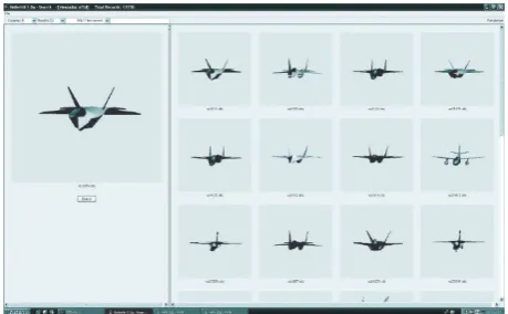
We managed to retrieve approximately 90% of the cars present in the database without any inlayer (precision: 100%; recall: 90%). This example shows that the proposed method can be applied, not only to identical objects submitted to a GCT, but also to similar or related objects. Comparable re-sults were obtained for planes and are illustrated inFigure 4. Most of the planes were retrieved without any inlayer, despite the fact that the resolution of the reference model was very low (precision: 100%; recall: 80%).

In our final example, we considerFigure 5which illus-trates a query for an animated body. Here, the woman’s arms are in two different positions. Such an animation cor-responds to a GCT.

Again, we managed to retrieve both postures without any inlayer. The next retrieved items (up to rank 250) were all human bodies without any inlayer (precision: 100%; recall: 100%). That shows, once more, that the method is invari-ant under general coordinate transformation and suitable to

Figure2: Retrieval of an animated 3D character: the reference ob-ject appears on the left side while the outcome of the query appears on the right side. Each result is characterised by a different facial expression, that is, a GCT. In the present query, all the facial ex-pressions of the character were retrieved without any inlayer from a database containing 12.150 objects.

Figure3: Retrieval of cars. Most of the cars (approximately 90%) were retrieved without inlayers from the 12.150 objects database. Only the first results are displayed.

Figure5: Retrieval of an animated 3D character. We retrieved all (i.e., 2) the postures associated with the mannequin and most of the human bodies from the 12.150 objects database. Only the first results are shown.

retrieve similar object while maintaining an adequate dis-crimination level.

The above-mentioned examples, as many others that are not shown in the present paper, indicate that the proposed method is efficient to retrieve 3D objects submitted to a GCT as well as similar objects from a large database. The fact that the database is large (12.150 objects) shows, at least from a statistical point of view, that the invariance under GCT does not compromise the level of discrimination of the algorithm.

8. CONCLUSIONS

In this paper, we have associated a curved space to an ar-bitrary object and have described this space with quantities that are invariant under general coordinate transformations. From those quantities we have built two representations: one based on the statistical distribution of the invariants and the other based on their topological distribution. Both represen-tations are invariant under GCT. Promising experimental re-sults were provided both analytically and numerically for a database of 12.150 3D objects.

To the best of our knowledge, there are no approaches that propose such a general and formal framework for GCT invariant representations of object. The next step will be to implement the proposed method, meaning solving exactly (27). This will be achieved through a foliation algorithm which will be implemented on a grid computer. In addition, I propose to study various approximations to (27) that would be precise enough for indexing and retrieval and that would facilitate and speed up the calculations.

REFERENCES

[1] N. Iyer, S. Jayanti, K. Lou, Y. Kalyanaraman, and K. Ramani, “Three-dimensional shape searching: state-of-the-art review and future trends,”Computer Aided Design, vol. 37, no. 5, pp. 509–530, 2005.

[2] J. W. H. Tangelder and R. C. Veltkamp, “A survey of con-tent based 3D shape retrieval methods,” inProceedings of IEEE

International Conference on Shape Modeling and Applications (SMI ’04), pp. 145–156, Genova, Italy, June 2004.

[3] A. Theetten, J.-P. Vandeborre, and M. Daoudi, “Determining characteristic views of a 3D object by visual hulls and Haus-dorffdistance,” inProceedings of 5th International Conference on 3-D Digital Imaging and Modeling, pp. 439–446, Los Alami-tos, Calif, USA, 2005.

[4] D. V. Vranic and D. Saupe, “Description of 3D-shape using a complex function on the sphere,” inProceedings of IEEE In-ternational Conference on Multimedia and Expo (ICME ’02), vol. 1, pp. 177–180, Lausanne, Switzerland, August 2002. [5] M. G¨ockeler and T. Sch¨ucker,Differential Geometry, Gauge

Theories, and Gravity, Cambridge University Press, New York, NY, USA, 1989.

[6] C. Rovelli, Quantum Gravity, Cambridge University Press, New York, NY, USA, 2004.

[7] C. Kiefer, Quantum Gravity, Oxford University Press, New York, NY, USA, 2004.

[8] D. Lovelock and H. Rund,Tensors, Differential Forms and Vari-ational Principles, Dover, New York, NY, USA, 1989.

[9] C. Bona and C. Palenzuela-Luque,Elements of Numerical Rel-ativity, Springer, New York, NY, USA, 2005.

[10] S. Wolfram,The Mathematica Book, Wolfram Media, Cham-paign, Ill, USA, 5th edition, 2003.

[11] C. P. Robert and G. Casella,Monte Carlo Statistical Methods, Springer, New York, NY, USA, 1999.

Eric Paquetis a Senior Research Officer at the Visual Information Technology (VIT) Group of the National Research Council of Canada (NRC). He received his Ph.D. de-gree in computer vision from Laval Univer-sity and the National Research Council in 1994. After finishing his Ph.D., he worked on optical information processing in Spain, on laser microscopy at the Technion-Israel Institute of Technology, and on 3D