R E S E A R C H
Open Access
Short range tracking of rainy clouds by
multi-image flow processing of X-band radar data
Luca Mesin
Abstract
Two innovative algorithms for motion tracking and monitoring of rainy clouds from radar images are proposed. The methods are generalizations of classical optical flow techniques, including a production term (modelling formation, growth or depletion of clouds) in the model to be fit to the data. Multiple images are processed and different smoothness constraints are introduced. When applied to simulated maps (including additive noise up to 10 dB of SNR) showing formation and propagation of objects with different directions and velocities, the
algorithms identified correctly the production and the flow, and were stable to noise when the number of images was sufficiently high (about 10). The average error was about 0.06 pixels (px) per sampling interval (ΔT) in
identifying the modulus of the flow (velocities between 0.25 and 2 px/ΔTwere simulated) and about 1° in
detecting its direction (varying between 0° and 90°). An example of application to X-band radar rainfall rate images detected during a stratiform rainfall is shown. Different directions of the flow were detected when investigating short (10 min) or long time ranges (8 h), in line with the chaotic behaviour of the weather condition. The algorithms can be applied to investigate the local stability of meteorological conditions with potential future applications in nowcasting.
Keywords:X-band radar, optical flow, nowcasting
1. Introduction
Quantitative precipitation monitoring and forecast is an important issue in water management, in flood forecast-ing, and in predicting hazardous conditions. Specific problems are the distinction of rain from snow [1], the monitoring of basins subject to floods or of areas prone to landslides [2], and the forecast of sudden rainfall over strategic regions, like as airports [3]. In these situations, detailed areal measurements of precipitation over a local spatial scale of range of a few tens of km and on a short time scale (e.g., 30 min, nowcasting) are needed.
For the remote sensing of rainfall, rain gauges dis-persed on the surface area of interest have been used. Nevertheless, they may be affected by gross mistakes, as wind, snowfall, drop size distribution influence the mea-sure. Moreover, a very dense network of gauges is needed, as the correlation between the measurements taken in two rain gauges is poor even at 500 m distance over time scales of 30 min [4].
As an alternative, radars may be used to study rainy clouds. Rainfall investigations have been usually con-ducted using S-band or C-band polarimetric radars, which use radiations with long wavelengths (about 10 and 5 cm, respectively) which allow for low attenuations [5]. These radar constellations are typically used for long range meteorological target detection. On the other hand, X-band radars can work only at short ranges and their radiations are significantly affected by attenuation behind heavy precipitation (due to the smaller wave-length, of about 3 cm). However, they have finer resolu-tion and smaller sized antennas than those required by S- or C-band radars, resulting in easier mobility and lower costs [6]. Moreover, using X-band radars has some advantages over S-band and C-band radars when investigating regions exhibiting a complex orography [4,7].
Radar images have been used for precipitation now-casting. Different techniques are based on correlation of successive images [8], on tracking the centroid of an object [9], and on the use of numerical prediction of wind advection [10]. Classical optical flow methods can Correspondence: [email protected]
Dipartimento di Elettronica, Politecnico di Torino, Corso Duca degli Abruzzi 24, Torino, 10129, Italy
estimate the motion of objects comparing a couple of subsequent images [11,12]. Some multi-frame techni-ques have also been introduced, in order to enhance robustness to noise and improve the discriminating cap-abilities of the algorithm [13,14]. When applied to preci-pitation forecasting [15,16], optical flow techniques track rainfall objects assuming that they remain constant in intensity (brightness constancy condition). On the other hand, shower clouds and the fine structure of stra-tiform rain bands can develop in a few minutes [17]. Their identification is not possible with classical optical flow techniques and their prediction is very difficult and requires detailed local information (which could be detected with X-band radars).
Other local weather forecast algorithms are based on the analysis of a few time-series representing meteorolo-gical variables like air temperature and humidity, visibi-lity distance, wind speed and direction, precipitation type and rate, cloud cover, and lightning [18]. Nonlinear prediction methods (e.g., based on artificial neural net-works models) usually compare the present condition with similar ones happened in the past and saved in a database. Nevertheless, meteorological variables have chaotic dynamics which could abruptly lead to comple-tely different conditions, even starting from similar ones [19,20]. The identification of stability or instability of the weather condition by a short range investigation could enhance the performances of local predictions by time-series analysis.
This article is devoted to the identification of forma-tion and propagaforma-tion of rainy clouds in short range, using data from an X-band radar. An innovative approach is proposed, based on classical optical flow theory, but estimating the formation and decay of rainy clouds in addition to their movements. This analysis can hardly be used for forecasting purposes, as the short spatial range investigated limits the time range of the reliable prediction, especially in the presence of fast rainy clouds or of showers. Nevertheless, it could pro-vide valuable indications on the stability or instability of weather conditions, which could feed a time-series based local model for rain prediction.
2. Methods
2.1. Description of experimental data
A new version of the X-band radar described in [4] was used. The radar transmits rectangular 10 kW peak power pulses (400 ns duration) at a frequency of 9.41 GHz, through a parabolic antenna with 3.6° beamwidth and 34 dB maximum gain. A maximum coverage of 30 km can be reached with an angular resolution of about 3° and a range resolution equal to 120 m.
Received power related to meteorological echoes within each single radar volume bin is converted into
the averaged reflectivity inside that volume. Two dimen-sional (2D) maps of reflectivity (Zin mm6m-3) are pro-vided as output to the pre-processing stage with a sampling interval of 1 min. Radar reflectivityZwas con-verted into rainfall rate R (measured in mm/h), using the Marshall and PalmerZ-Rrelation [21]
Z=ARb (1)
whereA andb are parameters that can be estimated by fitting experimental data from rain gauges placed on the area investigated by the radar. In this study, radar reflectivity data were converted into rainfall rates using the relation introduced in [22], fitting data of 7 years recorded in central Europe:
Z= 316R1.5. (2)
2.2. Mathematical model
Different radar images of rainfall rate can be compared to identify rainy clouds formation, growing or propaga-tion. Radar maps (within the considered time window) are modelled by the following equation
∂I(x,y,t) ∂t +
−
→v(x,y)· ∇I(x,y,t) =F(x,y) (3)
where I(x, y, t) is the intensity of the image as a function of the spatial coordinates (x, y) and time t (representing the radar reflectivity Z),
−
→v(x,y) = (v
1(x,y), v2(x,y)) is the velocity flow and F
(x, y) is a production term (which describes generation if positive, depletion if negative). The left hand side of Equation 3 is the total time derivative along the path of a propagating object of the image, that during its propa-gation may also vary its amplitude as an effect of the production termF(x, y). This model is quite general, but is based on assumptions which are not physical. For example, the distribution of clouds is 3D, whereas our model is 2D. Thus, the merging, intersection or growing of the available images of clouds could be the result of a complicated 3D motion. Thus, caution is needed in the interpretation of results.
In practice, both space and time variables are sampled. Thus, differential operators in Equation 3 are estimated within some approximation from sampled images. Velo-city flow and production term are assumed to be con-stant in the considered time window, which is sampled byNradar images.
It is not possible to solve directly optical flow pro-blems from two images, as two unknowns (the two components of the velocity flow) are to be estimated from one equation (aperture problem [24]). In the case of problem (3), the production term is a further unknown. Moreover, the production term could account for any time evolution of the image I(x, y, t) without including any flow −→v(x,y), leading to the trivial solu-tion
F= ∂I ∂t
−→v = 0. (4)
This problem is avoided when more than two images are included, assuming that both the velocity field and the production term are constant for all theNframes in the time window under consideration. This imposes that the motion of objects in different images is accounted for by the velocity field −→v(x,y) and the appearing, growth, depletion or extinction of objects determine the production termF(x, y).
2.3. Numerical implementation
The simplifying assumptions of the model and the ran-dom noise included in the experimental data impose that Equation 3 can apply only within some approxima-tions. For this reason, it is not expected that the para-meters of the model (i.e., −→v(x,y) and F(x, y)) can be estimated exactly, but only minimising the error with respect to the data. Given Nimages, the velocity field
−
→v(x,y) and the production term F(x, y) can be esti-mated optimally by solving the following mean square error problem
−→
v,F= arg min − →w,f
N−1
i=1
min(N,i+3)
j=i+1
Iijt +−→w · ∇Iij−f
2 2(5)
where ·2
2 indicates the square of the norm of the
space of square-integrable functions L2, Iijt = Ii−Ij
(i−j)dt the discrete version of the time derivative, withIi indicat-ing the ith reflectivity map and dt the time sampling
interval, Iij the radar map at the time sample i+j
2 dt
(the mean of the two closest maps was used wheni+j
2
was not an integer number), and ∇Iijthe gradient of Iij (estimated with a second order finite difference approxi-mation). It is worth noticing that in Equation 5 all pairs of maps were considered with maximal distance equal to 3. Including more maps lowers the effect of noise. On the other hand, when considering maps with
increasing delay, the finite difference approximation of model (3) is affected by an increasing error. For this rea-son, it is better to limit the time range of map pairs included in (5) (or, as an alternative, it is also possible to penalize the terms in the sum as a function of the delay between maps). Depending on the application and on the sampling frequency, the optimal maximal delay between maps should be properly chosen.
When time evolutions of the velocity field and of the production term are of interest, their estimation can be performed for a set of sliding time windows. Time evo-lutions are expected to be smooth, as the velocity field and the production term are computed assuming that they are constant for all the Nmaps in the considered time window.
In optical flow techniques, to avoid the aperture pro-blem, the velocity field is also constrained to be smooth in space [11,12]. This condition can be imposed either locally (requiring the flow to be constant in the neigh-bouring pixels of the considered one, Lucas and Kanede method [11]) or introducing global constraints of smoothness (Horn-Schunck method [12]).
2.4. Estimation of flow and production
In optical flow problems, in which the production term is not included, the brightness constancy condition together with spatial constraints are sufficient to esti-mate the flow even from two images. Such a flow was proven to reside in a low-dimensional linear space. Con-straining it to have the correct low number of degrees of freedom, noise content in the data can be reduced and a robust estimation of the flow can be obtained [13]. Two methods for the estimation of optical flow from a multi-frame analysis were recently introduced in [14] and compared to the technique proposed in [13]. The smoothness constraint was imposed locally (in line with Lucas-Kanede approach). Performances improved as the number of processed images increased. The two meth-ods were superior to that in [13] both in terms of com-putational cost and precision. The most precise method was based on the incremental difference approach, in which adjacent frames are used to estimate time deriva-tives, in line with Equation 5.
Both Lucas-Kanede [11] and Horn-Schunck
approaches [12] are here generalized to impose that the estimated velocity field and production term are smooth in space.
2.4.1. Lucas-Kanede approach
Within Lucas-Kanede framework, for each pixel of the image, the same equation was written for the M neigh-bouring pixels of the considered one. A Gaussian weighting factor (with standard deviation equal to 2√2
prominence to the central pixel and lower importance to more distant ones. For each pixel, the flow and the production terms were estimated in order to satisfy these multiple conditions optimally in the least square sense. Specifically, the following linear system was defined
AX = b X= ⎡ ⎢ ⎣ v1 v2 F ⎤ ⎥ ⎦ (6)
with the following definitions of the matrix Aand of the vectorb
As=
⎡ ⎢ ⎢ ⎣
w1Is
x(p1) w1Isy(p1) −w1 ..
. ... ...
wMIsx(pM) wMIsy(pM) −wM
⎤ ⎥ ⎥
⎦ A=
⎡ ⎢ ⎢ ⎣ A1 .. .
A3(N−2)
⎤ ⎥ ⎥ ⎦
bs=
⎡ ⎢ ⎢ ⎣ w1Is t(p1) .. .
wMIst(pM)
⎤ ⎥ ⎥
⎦ b=
⎡ ⎢ ⎢ ⎣ b1 .. .
b3(N−2)
⎤ ⎥ ⎥ ⎦
(7)
wherep1,...,pMis the set of neighbours of the
consid-ered point,w1,...,wMare the weights ands labels each of
the 3(N-2) pairs of maps (indicated by ijin Equation 5). In this article, 25 neighbours of each point were consid-ered (M = 25). Hence, for points located far from the boundary, the neighbours were located in a square with side 5, in line with [14]. The system (6) is over-deter-mined. The unknown vector Xwas estimated optimally in the least square sense by pseudoinversion (which pro-vides a close analytical solution to the problem).
2.4.2. Horn-Schunck approach
Following the Horn-Schunck method [12], the smooth-ness constraint is introduced by adding the energy norm of the gradients of the velocity flow and of the produc-tion term as regularizaproduc-tion components in Equaproduc-tion 3. Other constraints can be included, in order to introduce a-priori knowledge on the solution. For each map pair considered in Equation 5 (here labelled with s), the fol-lowing functional to be minimized was considered
Js(−→v,F) =Ist+−→v· ∇Is−F 2 2+α2
∇−→v22+∇F2 2
+β2F−→v2
2+γ2F22+δ2−→v 2 2 (8)
where α2∇−→v2
2 is the Horn-Schunck smoothness
constraint, α2∇F2
2 is an equivalent constraint for the
production term, β2F−→v2
2 reduces the correlation
between flow and production term (to force production and propagation terms to be present in different regions), γ2F2
2 and δ2−→v 2
2 limit the amplitude of
the two unknowns (Tikhonov regularization, [25]), in order that they do not become large to follow noise details.
The functional (8) can be minimized by solving the associated Euler-Lagrange equations [26]
⎧ ⎨ ⎩
(Is
t+−→v · ∇Is−F)Isx−α2v1+β2F2v1+δ2v1= 0
(Is
t+−→v · ∇Is−F)Isy−α2v2+β2F2v2+δ2v2= 0
−(Is
t+−→v · ∇Is−F)−α2F+β2F(v21+v22) +γ2F= 0
(9)
whereΔindicates the Laplacian operator. As proposed in [12], an iterative technique (Jacobi’s method) was applied to solve the system of equations (9). The non-linear terms F2v1, F2v2, and F(v21+v22) were estimated
from the previous step in the iteration. The Laplacian was expressed as
U=U−U (10)
where U is an average value estimated from the pre-vious step in the iteration. As time is sampled, Equa-tions 9 were written for each pair of maps considered to estimate the time derivative (refer to Equation 5). The following linear system of equations was obtained for thenth step of the iteration, for each pair of maps
⎡ ⎢ ⎢ ⎣ Is x
2+α2+δ2 Is xIsy −Isx Is
xIsy
Is y
2
+α2+δ2 −Is
y −Is
x −Isy 1 +α2+γ2
⎤ ⎥ ⎥ ⎦ ⎡ ⎣v n 1 vn 2 Fn ⎤ ⎦= ⎡ ⎢ ⎣ −Is
tIxs+α2v1n−1−β2(Fn−1) 2
vn−1 1
−Is
tIys+α2v2n−1−β2(Fn−1) 2vn−1
2
Is t+α2F
n−1−β2Fn−1((vn−1 1 )
2
+ (vn−1
2 ) 2
)
⎤ ⎥ ⎦. (11)
An estimation of the unknowns optimal in the least square sense was obtained by pseudoinverting the rec-tangular matrix containing the conditions (11) for each considered pair of maps. In order to facilitate conver-gence to smooth solutions, the flow and the production term estimated at each step of iteration were convolved with the Gaussian mask
1 16
⎡ ⎣1 2 12 4 2
1 2 1 ⎤
⎦. (12)
The following expressions were chosen for the para-meters in Equation 8
α= 0.25 exp−n5rms(∇I)β= 0.1 exp−n5rms(−→vn−1)
γ= 0.1 exp−n 5
rms(∇I) δ= 0.1 exp−n 5
rms(∇I) (13)
where n is the number of iteration, rms(∇I) is the average root mean square (RMS) of the gradients of the images and rms(−→vn−1) is the RMS of the vector flow estimated in the previous step of the iteration. As the iterations proceed, the values of the parameters decrease giving more importance to the fitting of data.
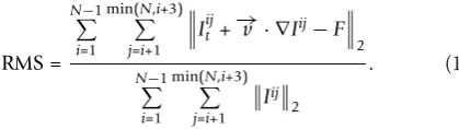
RMS =
N−1
i=1
min(N,i+3)
j=i+1
Iijt +−→v · ∇Iij−F
2
N−1
i=1
min(N,i+3)
j=i+1
Iij
2
. (14)
The algorithm proceeded as long as such an RMS error decreased. When the RMS error increased with respect to the previous step in the iteration, the algo-rithm was stopped and the estimated flow and produc-tion term at the previous step (i.e., the ones for which the RMS was minimum) were considered.
3. Results
The performance of the methods in tracking objects moving and growing in subsequent images was first tested in simulations. Then, some representative exam-ples of application to radar data are shown.
3.1. Simulated data
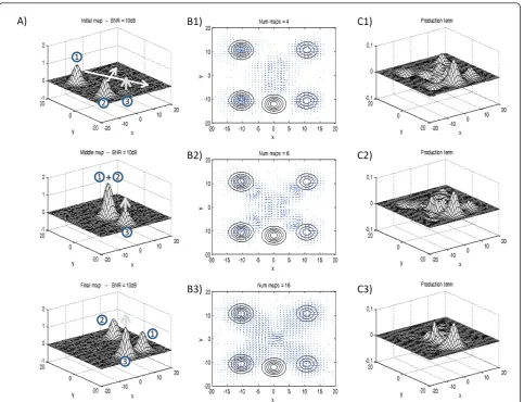
The reliability of the algorithms in tracking the motion and the growing up of 2D Gaussian functions was tested. In a preliminary test shown in Figures 1 and 2, two Gaussian functions were simulated to follow straight intersecting paths, whereas one Gaussian func-tion was growing at a rate of 0.1 per time sample. Speci-fically, the definitions of the three Gaussian functions are the followings
Gi(x,y,t) = exp
−(x−vxt−x0i)
2
+ (y±vyt−yi0)
2
2σ2
i= 1, 2
G3(x,y,t) =A(t) exp
−(x−x03) 2
+ (y−y0 3)
2
2σ2
A(t) = 0.1t (15)
whereGi(x, y, t) indicates theith Gaussian function, the first two propagating (at velocities (vx ± vy)), the third one remaining stationary, but growing at constant rate; moreover,(x0i,y0i)with i = 1, 2, 3 indicates the initial position of theith function. The initial conditions and the standard deviation (s= 2) of the three functions were chosen in order that their essential supports were separated in all considered images, except when the tra-jectories of the first two functions intersect (see Figure 1A). Additive Gaussian noise was included with signal to noise ratio (SNR) equal to 10 dB. No smoothing was performed before processing, even if the computation of numerical derivatives would improve by low pass filter-ing the images. Time was sampled with 16 images. It is worth noticing that the problem is not well posed, as the flow cannot be estimated in the points in which the first two Gaussian functions intersect.
Three experiments including a different number of images were performed. The initial and the final images were always considered. The other images were
under-sampled by a factor 5 (N= 4 images considered) or 3 (N= 6), or all of them (N= 16) were used to estimate the pro-pagation and growth of the three Gaussian functions. Fig-ure 1 shows results obtained using the algorithm based on the Horn-Schunck approach. Results indicate that using the minimum considered number of images (N= 4), the flow cannot be estimated: in such a case, the production term accounts for the disappearing of the first two Gaus-sian functions from their initial positions and their appear-ance in the final positions, with some contribution along their paths. Moreover, the growing of the third Gaussian function is identified. When increasing the number of images to 6, a local flow is estimated close to the initial and final positions of the first two Gaussian functions. The paths of the estimated flow are noisy and not straight. Moreover, the production term includes both the estimate of the growth of the third Gaussian function and some contribution along the paths of the two travelling ones. Including all the images, the estimation of the flow and of the production term is clear: the flow paths are straight and go from the initial to the final positions of the first two Gaussian functions; the production of the third Gaus-sian function is correctly estimated; the only residual pro-blem is in the region in which the paths of the first two Gaussian functions intersect, but in such a region the pro-blem is not well posed, as stated above.
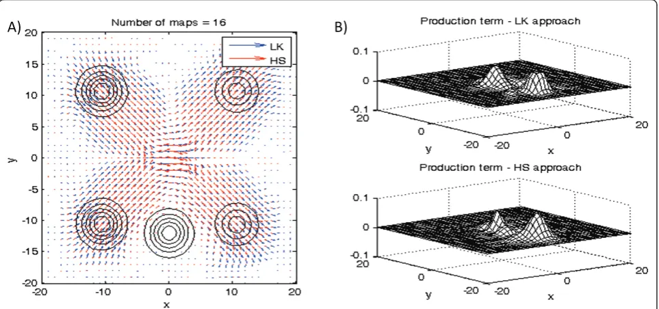
Figure 2 shows a comparison between the two imple-mented algorithms, considering the same simulations as in Figure 1, using 16 frames. Both Lucas-Kanede and Horn-Schunck approaches allows identifying the flow and the production term, with similar results (similar results are also obtained using the two different approaches with a lower number of frames).
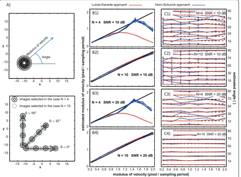
Different sets of simulated signals are considered in Figure 3 to investigate the performances of the algo-rithms in estimating the flux as a function of the modu-lus and direction of the propagation velocity and of the energy of additive random noise. A single propagating Gaussian function defined by an expression equal to that ofG1(x, y, t) in Equation 15 was considered (Figure
3A). Its motion was sampled by 10 images.
simulated modulus of velocity, superposing curves corre-sponding to different angles obtained averaging with respect to the noise realization and indicating the standard deviation (STD). In general, there is not an important effect of the angle on the estimated modulus of velocity.
Good estimates are obtained by both methods when the whole set of images is considered (Figure 3B2, B4). Using a small number of images (N = 4), the velocity can be estimated only if it is small (Figure 3B1, B3). Indeed, the estimates of the derivatives of the images with respect to the time and space variables are accurate only if the displacement is small (and only under the same condition the optical flow equations are justified [14]). Moreover, in the Lucas-Kanede approach, only small neighbours of each point are explored, so that the pairs of images contributing to the definition of matrix
A in Equation 6 could be not correlated within such small regions as the displacement of objects in different images is too large. On the other hand, Horn-Schunck method is based on global constraints and the Euler-Lagrange Equations 9 have a diffusion operator which contributes to coupling neighbouring points. It provides reliable estimates up to velocities of about 1.5 pixels per time sample. Thus, a proper choice of parameters (e.g., the extension of the neighbouring region in the Lucas-Kanede approach or the diffusion coefficient a2 in the Horn-Schunck approach) could help in following fast movements (as occurring when convective cells are pre-sent in the radar images). Nevertheless, increasing the sampling frequency is the best solution (e.g., in [14] dif-ferent methods were tested on a synthetic sequence manually generated by moving the images of the
1
2 3
1 2
3 +
1 2
3
A) B1)
B2)
B3)
C1)
C2)
C3)
sequence with the flow vector (0.1, 0.1) pixel/frame). Estimates of the angle of the velocity are depicted in Figure 3C as a function of the modulus and the angle of the simulated velocity, showing mean and STD of the estimates obtained with different realizations of noise. The direction of propagation is poorly estimated using a small number of images, even with a high SNR. The estimates are much more stable and precise when the number of images increases.
It is worth noticing that, as only propagation was simulated in this case, algorithms for optical flow avail-able in the literature could also be applied. The Lucas-Kanede algorithm for optical flow estimation, without including the production term, can be obtained substi-tuting the Equations 6 and 7 with the following
AX = b X=
v1
v2
(16)
where the matrixAand the vectorbare defined as
As=
⎡ ⎢ ⎢ ⎣
w1Ixs(p1) w1Isy(p1)
..
. ...
wMIsx(pM) wMIsy(pM)
⎤ ⎥ ⎥
⎦ A=
⎡ ⎢ ⎢ ⎣
A1
.. .
A3(N−2)
⎤ ⎥ ⎥ ⎦
bs=
⎡ ⎢ ⎢ ⎣
w1Ist(p1)
.. .
wMIst(pM)
⎤ ⎥ ⎥
⎦ b=
⎡ ⎢ ⎢ ⎣
b1
.. .
b3(N−2)
⎤ ⎥ ⎥
⎦.
(17)
Horn-Schunck algorithm for optical flow estimation, without including the production term, can be obtained substituting Equation 11 with the following
⎡ ⎣
Is x
2
+α2 Is xIsy
Is xIsy
Is y
2
+α2
⎤
⎦vn1
vn 2
=
−Is
tIsx+α2vn1−1
−Is tIys+α2v
n−1 2
. (18)
In general, their results are expected to be better than those obtained using the methods introduced here, in particular when the number of frames is small. Indeed, the new algorithms considered here have an additional degree of freedom (the production term) with respect to classical optical flow methods. Thus, for sets of images related only by flow, they need more information to learn that the production term is absent. Nevertheless, with the simulations considered here, the results are comparable, as shown in Table 1, where the errors in estimating velo-city and direction of the flow are indicated for the four methods (Horn-Schunck and Lucas-Kanede, including or excluding the production term), for each considered pair of values ofNand SNR. We can notice that the estimate of the modulus of the velocity is marginally affected by the intensity of the noise, whereas the estimation of the angle is less precise when the noise content increases.
For all the simulations considered in this paper, the number of iterations required by the Horn- Schunck algorithm to converge was about 5 to 10 and the RMS error in fitting the data (defined in Equation 14) was between 5 and 15% for all the methods considered.
A)
B)
3.2. Application to experimental data
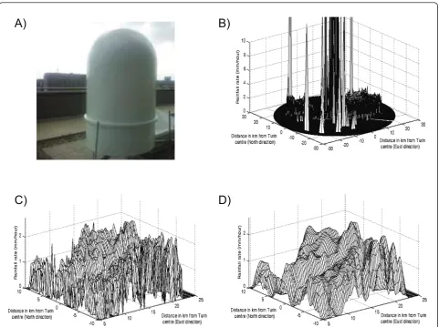
As an example of application, the meteorological condi-tions during the night (from 23:00 to 7:00) between the 20th and the 21th of November, 2010 were considered. Rainfall rate was estimated using data detected from the X-band radar described in Section 2.1 and shown in Fig-ure 4A, placed on the roof of Politecnico, close to the centre of Turin. The first considered map of rainfall rate is shown in Figure 4B. The spikes are associated to clut-ters. Data were re-sampled in order to convert the polar coordinates into Cartesian ones, with homogeneous sampling with resolution 500 m. Moreover, maximum rainfall rate considered was 10 mm per h. Experimental values larger than such a limit (assumed to correspond to clutters) were removed and their value was computed by linear interpolation. A square region centred 15 km at East of the centre of Turin and with side 20 km was
considered (Figure 4C). Before processing, experimental noise was reduced by a spatial low pass filter obtained by 2D convolution with a Gaussian mask with standard deviation equal to 500 m, as shown in Figure 4D.
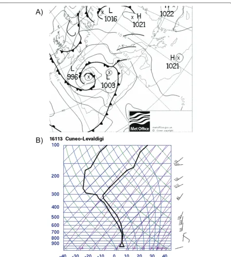
The case study concerns a stratiform rain fallen on Turin. From the meteorological analysis, low pressure in the South of France entailed a cyclone circulation: wind fields at 500 hPa (height of clouds responsible of preci-pitation) move from South to North in Northern Italy, as noticeable from MetOffice pressure map (Figure 5A) and Cuneo-Levaldigi radio-sounding station near Turin (Figure 5B).
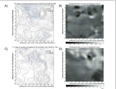
Figure 6 shows two examples of estimation of the flow and production of rainy clouds by the proposed algo-rithm based on the Horn and Schunck approach. The square region on the East of Turin shown in Figure 4C, D was studied. Two time ranges were considered: 10
est
imat
ed
m
odul
us
of
v
el
oci
ty
(pi
xel
/
sampl
ing
peri
od)
x y
-15 -10 -5 0 5 10 15 -15
-10 -5 0 5 10 15
Angle
Images selected in the case N = 4
Images selected in the case N = 10
x y
-15 -10 -5 0 5 10 15 -15
-10 -5 0 5 10 15
T q
T q
T q A)
0.2 0.4 0.6 0.8 1.0 1.2 1.4 1.6 1.8 2.0 1
2
modulus of velocity (pixel / sampling period) N = 10 SNR = 20 dB
1 2
N = 4 SNR = 20 dB
1 2
N = 10 SNR = 10 dB
1 2
N = 4 SNR = 10 dB
10 30 50 70 90 10 30 50 70 90
esti
ma
ted
angl
e (
)
10 30 50 70 90
10 30 50 70 90
0.2 0.4 0.6 0.8 1.0 1.2 1.4 1.6 1.8 2.0 0
0
0
0
B1)
B2)
B3)
B4)
N=4 SNR = 10 dB C1)
N=10 SNR = 10 dB C2)
N=10 SNR = 20 dB
C4)
C3) N=4 SNR = 20 dB
Lukas-Kanede approach Horn-Schunck approach
min sampled by 10 radar maps (Figure 6A, B) and 8 h sampled by 17 maps of cumulative rainfall rate, each obtained adding sampled images for 30 min (Figure 6C, D). The estimated flows are shown on the left (Figure 6A, C). The flow averaged over the longer time range
(Figure 6C) is predominantly directed upward, in North-East direction, in agreement with the indications of the MetOffice pressure map (Figure 5A). On the other hand, the flow estimated from the radar maps recorded during the specific short time period shown in Figure
A)
C)
B)
D)
Figure 4(A) Picture of the X-band radar on the roof of Politecnico, in Turin.(B)Rainfall rate estimated from the measured reflectivity (the range of rainfall rate was limited to 10 mm per hour; spikes correspond to clutters).(C)Rainfall rate in a region in the East of Turin selected for further processing.(D)Smooth rainfall rate computed from the image in(C)by low pass filtering with a Gaussian mask with standard deviation equal to 1 pixel.
Table 1 Absolute error in estimating modulus and phase of the flow
Simulation parameters Lucas-Kanede approach Horn-Schunck approach
Modulus (px/ΔT) Angle (°) Modulus (px/ΔT) Angle (°)
F No F F No F F No F F No F
N= 4, SNR = 10 dB 0.58 ± 0.62 0.49 ± 0.54 1.0 ± 1.7 0.6 ± 0.7 0.50 ± 0.59 0.41 ± 0.42 2.3 ± 2.0 2.2 ± 1.7
N= 4, SNR = 20 dB 0.58 ± 0.60 0.49 ± 0.53 0.9 ± 1.8 0.5 ± 1.7 0.49 ± 0.57 0.39 ± 0.40 1.8 ± 1.9 1.7 ± 1.5
N= 10, SNR = 10 dB 0.06 ± 0.03 0.04 ± 0.04 0.2 ± 0.2 0.2 ± 0.2 0.06 ± 0.03 0.07 ± 0.08 2.4 ± 3.3 1.7 ± 1.9
N= 10, SNR = 20 dB 0.05 ± 0.04 0.04 ± 0.03 0.2 ± 0.2 0.2 ± 0.2 0.06 ± 0.03 0.07 ± 0.08 0.7 ± 0.6 0.7 ± 0.5
6A is predominantly directed downward, in South direc-tion, opposite to the indications of the MetOffice pres-sure map and to the average flow estimated processing a time period covering the majority of the event (Figure 6C). Moreover, the motions of clouds appear to be
more turbulent and discontinuous (i.e., with large spatial variations) when a short time range is considered. The estimated productions of rainy clouds are shown on the right of Figure 6 (in 6B and 5D). The production is lower when the time range is larger, probably due to the
A)
B)
low pass filter effect of cumulating the rainfall rate. Such a procedure has the effect of smoothing out the differ-ences between successive maps, which are identified by the algorithm as production or extinction of clouds (if they are not moving).
All radar maps presented a still local maximum, which is a clutter, centred about 19 km East and 5 km North of Turin. The estimated flow and production term van-ish close to such a region.
The number of iterations required by the algorithm to converge was about 5 to 10 when processing 10 maps sampled every minute. In such a case, the RMS error (defined in Equation 14) was between 5 and 10%. Processing the 17 maps of rainfall rate cumulated every 30 min required 12 iterations; the RMS error in fitting the data was 1.2%.
4. Discussion and conclusions
Two innovative algorithms are proposed to track rainy clouds motion and to identify their generation and loss. The methods are based on the classical Lucas-Kanede [11] and Horn-Schunck [12] optical flow techniques, but estimate also a production term accounting for the appearance, growing, depletion, or extinction of objects in subsequent images. This requires the inclusion of more than two images in the processing.
The two methods have comparable performances when applied to simulated signals (Figures 2 and 3). Moreover, when applied to a set of images satisfying the bright constancy condition, their performances are simi-lar to those of multi-frame versions of classical optical flow techniques (Table 1).
A)
C)
B)
D)
An important parameter affecting performances is the number of images processed by the algorithms (Figures 1 and 3). Including an increasing number of images makes the results more and more stable to random noise. Indeed, a single flow and a single production term are estimated out of more noisy images, extracting average properties (i.e., the motion and the generation of objects) which consistently appear in different images, and reducing the effect of random fluctuations. Flow and production term estimated from sets of simulated images with constant flow and generation improved when the number of processed images increased (Fig-ures 1 and 3 and Table 1). On the other hand, increas-ing the number of images keepincreas-ing constant the sampling interval increases the time range of investiga-tion. As the algorithms assume that the flow and the generation of objects do not change within the pro-cessed images, increasing the investigation interval reduces their capability to detect rapid variations devel-oping at a shorter time scale. Thus, a proper over-sam-pling related to the time scale of the phenomenon of interest is needed for a correct application of the meth-ods. Over-sampling is more important for the Lucas-Kanede approach, as the smoothness constraint is imposed locally.
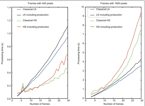
The methods were implemented in Matlab, on a Pen-tium(R) Dual-Core, with clock frequency of 2.8 GHz, 4 GB of RAM and 64 bits operating system, using routines running on a single core. The computational cost is shown in Figure 7 in terms of the processing time as a function of the number of frames, in the case of images with different dimensions (notice the erratic processing time corresponding to the Horn-Schunck approach, which depends on the number of iterations needed to converge). The computational cost increases rapidly with the dimension of the frame and with the number of images considered. The inclusion of the production term increases marginally the processing time. The algo-rithms are feasible for parallel implementation, as the same steps should be repeated for each pixel in the image. Moreover, using an optimized implementation and a compiled language could significantly reduce the processing time. Thus, processing about 10 to 20 frames with dimension similar to those considered here, the algorithms could process data in (quasi) real time. Nevertheless, this is not strictly needed for the specific application on meteorological nowcasting.
The algorithm generalizing the Horn-Schunck approach includes many parameters which could be properly chosen in order to fit the specific application. Four parameters give to the user the possibility to weight properly some constraints which facilitate the convergence of the algorithm toward a solution with smoothness properties defined a-priori. In this work,
such parameters were fine tuned by a trial and error approach. A slow reduction of the parameters for each iteration of the algorithm provided reliable results.
A representative example of application to rainy clouds tracking is shown in Figures 4 to 6. A stratiform rainfall event with main stream from South to North was investigated. When a long portion (8 h long) of the event was investigated using images of cumulated rain-fall rate, the main direction of the estimated flow agreed with the indications of the MetOffice pressure map. Nevertheless, it was possible to identify a local flow in the opposite direction when a shorter time range (10 min long) was considered. Moreover, dynamics were more irregular in space when the investigated time range was shorter. These experimental observations are in line with the nonlinear and chaotic dynamics charac-terizing the meteorological variables [20]. Indeed, the equations governing the temporal evolution of weather are a series of partial differential equations with chaotic solutions, showing self-similar (fractal) geometry [27]. This implies that similar variations of flow can be observed at different spatial scales (becoming more and more complicated and discontinuous as the spatial scale is reduced). Moreover, similar past events could evolve into very different conditions, as already noted in [28]. Indeed, small differences in the conditions measured in a point can be amplified by the nonlinear dynamics. The Lyapunov exponent is a measure of the rate of exponen-tial divergence of trajectories starting from neighbouring points [29]. When forecasting weather dynamics, predic-tion horizon is usually very short, especially in unstable conditions, and related to the inverse of the Lyapunov exponent [30] characterizing the chaotic system.
meteorological variables measured in the location in which the forecast is of interest. The prediction is not based on a simple linear extension of the present condi-tions, but on a nonlinear algorithm comparing the actual state with similar ones found in the past [29,31]. However, local variables usually contain poor informa-tion about the stability or instability of weather condi-tions, which is important to perform a reliable forecast. Indeed, predicting the onset or the duration of rainy events from local measurements is very difficult, as it requires identifying the transition between two comple-tely different weather states. The task could benefit from some specific indication extracted from a short range investigation indicating if the weather is stable or not. The algorithm presented here could provide infor-mation about the presence of rainy clouds in the vicinity of the local position of interest, their movements (possi-bly related to the wind at high altitude), which could be
turbulent or stationary, and cloud formation and grow-ing. All this information could be converted into a set of scalar time-series feeding a predictor model, together with the other time series already used, in order to improve the reliability of the forecast.
List of abbreviations
RMS: root mean square; SNR: signal to noise ratio; STD: standard deviation; 2D: two dimensional.
Acknowledgements
This work was sponsored by the national project AWIS (Airport Winter Information System), funded by Piedmont Authority, Italy. The author is deeply indebted to Riccardo Notarpietro and Andrea Prato for their interesting comments and suggestions.
Competing interests
The authors declare that they have no competing interests.
Received: 13 May 2011 Accepted: 19 September 2011 Published: 19 September 2011
0 5 10 15 20 25 30
0 1 2 3 4 5 6 7 8 9 10
Number of frames
Pr
ocessi
ng
ti
me
(s
)
Frames with 1600 pixels
0 5 10 15 20 25 30
0.0 0.2 0.4 0.6 0.8 1.0 1.2 1.4
Number of frames
Pr
ocessi
ng
ti
me
(s
)
Frames with 400 pixels
Classical LK
LK including production
Classical HS
HS including production
Classical LK
LK including production
Classical HS
HS including production
References
1. SE Giangrande, AV Ryzhkov, Polarimetric method for bright band detection, inProceedings of the 11th Conference on Aviation, Range, and Aerospace
(2004)
2. J Schmidt, G Turek, MP Clark, M Uddstrom, JR Dymond, Probabilistic forecasting of shallow, rainfall-triggered landslides using real-time numerical weather predictions. Nat Hazards Earth Syst Sci.8, 349–357 (2008). doi:10.5194/nhess-8-349-2008
3. A Klein, S Kavoussi, RS Lee, Weather forecast accuracy: study of impact on airport capacity and estimation of avoidable costs, inEighth USA/Europe Air Traffic Management Research and Development Seminar, (2009)
4. M Gabella, F Orione, M Zambotto, S Turso, R Fabbo, A Pillon, A portable low cost X-band RADAR for rainfall estimation in Alpine valleys: Analysis of RADAR reflectivities and comparison between remotely sensed and in situ measurements; Test of a prototype in Friuli Venezia Giulia. FORALPS Technical Report 3 (2008)
5. G Delrieu, H Andrieu, JD Creutin, Quantification of path-integrated attenuation for X- and C-band weather radar systems operating in Mediterranean heavy rainfall. J Appl Meteorol.39, 840–850 (2000). doi:10.1175/1520-0450(2000)0392.0.CO;2
6. SG Park, VN Bringi, V Chandrasekar, M Maki, K Iwanami, Correction of radar reflectivity and differential reflectivity for rain attenuation at × band. Part I: theoretical and empirical basis. J Atmos Oceanic Tech.22, 1621–1632 (2005). doi:10.1175/JTECH1803.1
7. M Gabella, R Notarpietro, S Turso, G Perona, Simulated and measured X-band radar reflectivity of land in mountainous terrain using a fan-beam antenna. Int J Remote Sens.29(10), 2869–2878 (2008) (2008). doi:10.1080/ 01431160701596149
8. A Bellon, GL Austin, The evaluation of two years of realtime operation of a short-term precipitation forecasting procedure (SHARP). J Appl Meteorol. 17(12), 1778–1787 (1978). doi:10.1175/1520-0450(1978)0172.0.CO;2 9. JT Johnson, PL Mackeen, A Witt, ED Mitchell, GJ Stumpf, MD Eilts, KW
Thomas, The Storm cell identification and tracking algorithm: an enhanced WSR-88D algorithm. Weather Forecast.13, 263–276 (1998). doi:10.1175/ 1520-0434(1998)0132.0.CO;2
10. DB Parsons, PV Hobbs, The mesoscale and microscale structure of cloud and precipitation in midlatitude cyclones, XI, comparison between observational and theoretical aspects of rainbands. J Atmos Sci.40, 2377–2397 (1983). doi:10.1175/1520-0469(1983)0402.0.CO;2
11. BD Lucas, T Kanade, An iterative image registration technique with an application to stereo vision, inProceedings of Imaging Understanding Workshop, 121–130 (1981)
12. BKP Horn, BG Schunck, Determining optical flow. Artif Intell.17, 185–203 (1981). doi:10.1016/0004-3702(81)90024-2
13. M Irani, Multi-frame optical flow estimation using subspace constraints, in
Proceedings of the Seventh IEEE International Conference on Computer Vision, 1, 626–633 (1999)
14. C-M Wang, K-C Fan, C-T Wang, Estimating optical flow by integrating multi-frame information. J Inform Sci Eng.24, 1719–1731 (2008)
15. NEH Bowler, CE Pierce, A Seed, Development of a precipitation nowcasting algorithm based upon optical flow techniques. J Hydrol.288, 74–91 (2004). doi:10.1016/j.jhydrol.2003.11.011
16. M Peura, H Hohti, Optical flow in radar images, inEuropean Conference on Radar in Meteorology and Hydrology (ERAD2004), Copernicus, 454–458 (2004) 17. JW Wilson, NA Crook, CK Mueller, J Sun, M Dixon, Nowcasting
thunderstorms: a status report. Bull Am Meteorol Soc.79(10), 2079–2099 (1998). doi:10.1175/1520-0477(1998)0792.0.CO;2
18. E Pasero, W Moniaci, T Meindl, A Montuori, NeMeFo: Neural meteorological forecast, inSIRWEC 12th International Road Weather Conference, Bingen (EU-D), Paper Topic II-4 (2004)
19. L Mesin, F Orione, E Pasero, Nonlinear adaptive filtering to forecast air pollution, inAdaptive Filtering, ed. by Morales LG (Intech, Rijeka, Croatia, 2011)
20. AA Tsonis, The impact of nonlinear dynamics in the atmospheric sciences. Int J Bifurc Chaos.11, 881–902 (2001). doi:10.1142/S0218127401002663 21. JS Marshall, WM Palmer, The distribution of raindrops with size. J Meteor.5,
165–166 (1948). doi:10.1175/1520-0469(1948)0052.0.CO;2
22. IG Doelling, J Joss, J Riedl, Systematic variations of Z-R relationships from drop size distributions measured in northern Germany during seven years. Atmos Res.47-48, 635–649 (1998)
23. JO Limb, JA Murphy, Estimating the velocity of moving images in television signals. J Clin Neurophysiol.4, 311–327 (1975)
24. DJ Fleet, Y Weiss, Optical flow estimation, inMathematical models for Computer Vision: The Handbook, ed. by Paragios N, Chen Y, Faugeras O (Springer, New York, USA, 2005), pp. 239–258
25. HW Engl, M Hanke, A Neubauer,Regularization of Inverse Problems(Kluwer, Dordrecht, 1996)
26. R Courant, D Hilbert,Methods of Mathematical Physics(Interscience, New York, 1953)
27. S Lovejoy, BB Mandelbrot, Fractal properties of rain, and a fractal model. Tellus.37A, 209–232 (1985). doi:10.1111/j.1600-0870.1985.tb00423.x 28. EN Lorenz, Deterministic nonperiodic flow. J Atmos Sci.20(2), 130–148
(1963). doi:10.1175/1520-0469(1963)0202.0.CO;2
29. H Kantz, T Schreiber,Nonlinear Time Series Analysis(Cambridge University Press, Cambridge. United Kindom, 1997)
30. S Haykin,Neural Networks: A Comprehensive Foundation(Pearson Education, Dehli, India, 1999)
31. E Pasero, W Moniaci, Artificial neural networks for meteorological nowcast. inProceedings of CIMSA 2004, IEEE Conference on Computer Intelligence for Measurement Systems and Applications(Boston, MA, USA, 2004), pp. 36–39
doi:10.1186/1687-6180-2011-67
Cite this article as:Mesin:Short range tracking of rainy clouds by multi-image flow processing of X-band radar data.EURASIP Journal on Advances in Signal Processing20112011:67.
Submit your manuscript to a
journal and benefi t from:
7Convenient online submission 7Rigorous peer review
7Immediate publication on acceptance 7Open access: articles freely available online 7High visibility within the fi eld
7Retaining the copyright to your article