Volume 2011, Article ID 806516,12pages doi:10.1155/2011/806516
Research Article
Image Informative Maps for Estimating Noise
Standard Deviation and Texture Parameters
M. Uss,
1, 2B. Vozel,
1V. Lukin,
3S. Abramov,
3I. Baryshev,
2and K. Chehdi
11TSI2M Laboratory, University of Rennes 1, BP 80518, 22305 Lannion cedex, France
2Department of Design of Aircraft Radio-Electronic Systems, National Aerospace University (Kharkov Aviation Institute),
17 Chkalova Street, 61070 Kharkov, Ukraine
3Department of Receivers, Transmitters and Signal Processing, National Aerospace University (Kharkov Aviation Institute),
17 Chkalova Street, 61070 Kharkov, Ukraine
Correspondence should be addressed to B. Vozel,[email protected]
Received 7 December 2010; Accepted 21 February 2011
Academic Editor: Joao Manuel R. S. Tavares
Copyright © 2011 M. Uss et al. This is an open access article distributed under the Creative Commons Attribution License, which permits unrestricted use, distribution, and reproduction in any medium, provided the original work is properly cited.
The problem of automatic detection of image areas appropriate for accurate estimation of additive noise standard deviation (STD) irrespectively to processed image properties is considered in this paper. For accurate estimation of either image texture or noise STD, we distinguish two complementary informative maps: noise- (NI-) and texture- (TI-) informative ones. The NI map is determined and iteratively upgraded based on the Fisher information on noise STD calculated in scanning window (SW) fashion. Fractional Brownian motion (fBm) model for image texture is used to derive the required Fisher information. To extract final noise STD from NI map, fBm- and DCT-based estimators are implemented. The performance of these two estimators is comparatively assessed on large image database for different noise levels. It is also compared with performance of two competitive state-of-the-art estimators recently published. Utilizing NI map along with DCT-based noise STD estimator has proved to be significantly more efficient.
1. Introduction
Images formed by multispectral sensors or digital cameras are subject to undesirable errors including sensor ran-dom noise, blur, distortions, radiometrical, and geometrical errors. These effects are to be detected and quantified, either prior to subsequent image processing, aiming at their com-pensation (filtering or deblurring) or prior to image low level information extracting [1]. Sensor random noise is often a dominant factor degrading image quality [1–3]. Although there are methods that are able to perform image processing (segmentation, denoising, edge detection, classification, etc.) without using a priori knowledge or pre-estimating noise STD (segmentation methods [4,5] are interesting examples of such methods), better performance is usually provided for techniques that exploit such a priori information or estimation of noise STD [6]. For example, BM3D filer, one of the best filters available today [7], requires noise STD to be known or pre-estimated [8].
It is often desirable to estimate noise STD in a blind manner. First of all, blind processing allows dealing with a large amount of data acquired by modern sensors. Second, potentially, performance of blind methods is higher than that of a human operator, as they may use subtle difference between image content and noise that can be not visible for a human eye. To reach good performance in practice, a blind estimator of noise STD should satisfy the following requirements [2]: (1) to provide unbiased estimates with variance as small as possible; (2) to perform well enough at different noise levels; (3) to be not sensitive to image content, that is, to provide appropriate accuracy even for textural images. These requirements are controversial and it has been found a difficult problem to satisfy them altogether.
STD. Indeed, it is preferable to use those areas where signal and noise can be quite easily separated. The easiest situation for benefiting from such separation is maybe in the spatial domain. Spatial methods make essential use of the processed image areas with negligible level of texture spatial variation compared to the noise level, so-called homogeneous areas (HA) [3]. As HAs hypothesis could be quite restrictive due to a limited area of HAs within processed images (authors of the paper [9] reported 0.6–2% of HAs in Visible InfraRed Scanner, VIRS-200, hyperspectral image), spatial methods may fail to provide practically desired accuracy, and may result in biased noise STD estimates [10] (see results of testing method [11] by Roger and Arnold in [12]). To get around these shortcomings, methods operating in the spectral domain utilize the fact that image texture is known to be usually smoother than noise. As a result, after applying suitable decorrelation transform, texture is concentrated in low frequency transform coefficients in contrast to the noise which spreads uniformly among low and high transform coefficients (for spatially uncorrelated noise). DCT [13], 3D DCT [14], and wavelet [15,16] transforms have been selected for this purpose in the past.
Typically, positions of HAs or nonintensive texture areas are not known in advance [9]. And using nonappropriate textural areas (even nonintensive ones) for noise STD estimation may lead to outliers that can degrade the final noise STD estimate. Performance reduction of both spatial and spectral state-of the-art estimators for textural images [10] is mainly explained by aforesaid reason. Two different ways to cope with this problem have been proposed so far. The first one is to consider the whole image for noise STD estimation and to reject outliers that come from textural areas by a robust postprocessing of local estimates [9]. The main idea consists in splitting an image into small fragments, calculating for them local means and local STDs [11,17]. Then the final noise STD can be estimated either by robustly fitting linear model to the corresponding scatter plot [18] or by robust finding the histogram mode of local variance estimates [11, 19]. However, this approach fails to provide accurate estimates if HAs and areas with nonintensive texture cover less than 10–20% of the image [20].
The second approach is to consider complementary pre-classification to preliminary determine suitable areas (either HAs or nonintensive texture areas) [21]. In paper [22], HAs are selected interactively and manually for hyperspectral images. But this task is not so easy for large and complex images and can lead to erroneous selections. Besides it is labor consuming and requires qualified operators. Automatic classification of the processed image into textural and homo-geneous areas [23] or the Automated Local Convergence Locator (ALCL) proposed in [24] can be considered for both facilitating and improving HAs selection accuracy [23]. When the obtained classification is effective enough, these processing stages can contribute to improve the performance of a noise STD estimation method as it was shown for method [19] for textural images [25].
However, classification methods may also fail to discrimi-nate correctly between areas appropriate and nonappropriate
for noise STD estimation, because of the textured features of the processed image and/or the noise level. In this case, the discrimination errors lead to outliers and to performance degradation of the whole procedure, including classification and noise STD estimation itself. As a result, preclassification and robust postprocessing stages are to be used simultaneously [21].
This paper concentrates on the problem of blind estimation of sensor random noise STD from noisy textured images. The noise is assumed additive signal-independent and uncorrelated (i.i.d). Although this model is slightly ide-alized, it is widely used for images formed by old generation hyperspectral sensors, color images, and so forth [26]. In this paper, we propose and describe a new estimation scheme that belongs to the preclassification approach mentioned above. Our main goal is to demonstrate the proposed approach ability to significantly improve noise STD estimation accu-racy over the state of the art. That is why we have restricted ourselves to additive noise case for which sophisticated estimators have been proposed and simulation results are available in the literature. Note that our approach is not limited to the additive noise case; the same formalism can be followed for signal-dependent noise as well as for correlated noise.
In our approach, we mainly deal with textural images and texture parameters are estimated as well but only as a support for the main problem of noise STD estimation. The approach novelty is that it presumes finding image NI and TI areas where information is understood in Fisher’s statistical sense. All detected TI and NI areas compose, respectively, the two complementary TI and NI maps, further used to discriminate suitable SW for estimating either noise or texture parameters. For each image SW, we calculate Fisher’s information (or Cram´er-Rao Lower Bound, CRLB) on noise STD. Then, the SWs are sorted according to their decreasing level of information on noise STD (increasing CRLB). All SWs with information above a threshold compose NI map and the rest of them compose TI map. Thus, each SW that belongs to NI map can provide a noise STD estimate with predefined accuracy making this map especially useful for contributing to final noise STD estimation. The proposed CRLB-based approach also allows estimating potential accuracy of noise STD estimates for any single SW and for the whole NI map as well.
In contrast to some classification (or segmentation) methods where the goal is to classify image content well enough independently (under some conditions) on unknown noise level [4,5], our objective, given any noise level, is not to classify image content, but simply to obtain two complementary maps. One map is intended for accurate noise estimation, the other one; for accurate image texture model estimation. In our application, for different noise levels, different NI and TI maps will be (and should be) obtained.
is a function of texture and noise parameters that are both unknown. To be effective, this CRLB-based criterion needs to be accurately estimated from a noisy image. The problem is that it is usually difficult to estimate texture parameters from a noisy image on one hand and noise parameters from textural image on the other hand. Indeed, starting with an initial guess for the NI and TI maps, we can expect ourselves to accurately estimate texture parameters from TI map by fixing noise STD (optimistically to a value close to the true one) and noise STD from NI map by fixing texture parameters (optimistically to a vector value close to the true one). But we can hardly expect to accurately estimate both of them from any SW in the whole image. To solve this practical issue, we propose to predict unknown texture parameters for NI map and noise STD for TI map by values estimated from the respective complementary maps. By doing this, we hope to obtain quite accurate estimates of texture and noise parameters available for any SW in the whole image. Based on this knowledge, both informative maps can be in turn refined and upgraded by considering CRLB-based criterion once again. These two stages are iterated for refining texture parameters and noise STD estimates as well as respective informative maps until convergence criterion is reached.
In practice, our method follows a nonlocal approach with respect to involved parameters. In this, it differs from the approach in paper [14] where the same nonlocal approach is used with respect to similar texture patches, as this is basically exploited in image filtering [27].
We consider 2D fBm-model for describing image texture with the Hurst exponent,H, translating texture roughness (correlation structure). We assume that in a neighborhood of an image pixel, texture Hurst exponent (roughness) varies only a little. On the contrary, texture amplitude can vary significantly (change in light conditions is an example), and it is possible to find both TI and NI SWs within image local neighborhood. This assumption, though simple (e.g., it does not take into account image edges), allows developing maximum likelihood (ML) noise STD estimator and confirming the practical interest of using TI and NI maps as additional sources of useful information on both texture and noise local parameters.
It is important to note that noise STD estimation is emphasized in the proposed scheme, though texture param-eters (roughness and amplitude) according to the fBm model are also estimated for the whole image. These estimates can be useful for quantifying and classifying image textures [28].
This paper is organized as follows.Section 2introduces the fBm-field model and details of the proposed scheme based on NI and TI maps to improve texture and noise parameters estimation accuracy. We introduce Fisher infor-mation on noise STD in a single SW and explain how it is utilized for building NI and TI maps. Specific estimators are defined for texture parameters and noise STD in, respectively, NI and TI maps. In Section 3, we comparatively assess the proposed noise STD estimators on large database of real-life images with other state-of-the-art estimators. Finally, in Section 4, we conclude the work.
2. Noise STD Estimation Based on Texture- and
Noise-Informative Maps
2.1. The Proposed Approach. We denote by y(t,s) an observed image for which we assume additive noise model
y(t,s)=x(t,s) +n(t,s), (1)
wherex(t,s) is the corresponding noise-free image at pixel position (t,s) andn(t,s) is a normally distributed spatially uncorrelated random field with zero mean and varianceσ2
n. When solving the problem of blind noise STD estimation in anN×NSW fashion, we would like to determine which SWs should be used for noise STD estimation and which should be rejected. Let us discuss this task from the Fisher’s information point of view. We assign a Fisher’s information for noise STD estimation ISTD to each SW. By setting a
threshold on ISTD, it is possible to divide all image SWs
into two groups: (1) SWs withISTDabove the threshold and
(2) SWs withISTD below the threshold. The first group of
SWs corresponds to HAs or areas with nonintensive texture that allow to accurately estimate noise STD, provided texture parameters are known. Thus, we call them NI SWs. The second group of SWs corresponds to textural areas. Such areas are noninformative for noise STD estimation, but they are able to provide helpful and quite accurate information on image texture parameters. Thus we call them TI SWs. All NI and TI SWs compose NI and TI maps, respectively.
Only those SWs that belong to the NI map should be basically used for noise STD estimation (see discussion below in Section 2.3). The use of SWs from the TI map would lead to overbiased estimates due to strong outliers [2]. As image areas that correspond to NI and TI maps are not known in advance, finding NI SWs is a crucial primary task for blind noise parameters estimation. To solve this problem, ISTD should be estimated in SWs fashion
directly from noisy image. Note that Fisher information is a function of both texture and noise true parameters which are all unknown. Unfortunately, these parameters cannot be accurately estimated from a single SW: a given informative map can only provide accurate estimates either for texture parameters or noise STD.
To overcome this difficulty, we propose on one hand, to predict texture parameters in NI map with parameters estimated from neighboring TI map. On the other hand, noise STD in TI map is to be estimated from NI map (see
Figure 1). By making use of such an alternative estimation
scheme, it seems possible to estimate quite accurately both noise and texture parameters for the whole image allowing reliable Fisher information calculation and further discriminating between NI/TI SWs.
Texture-informative areas Noise-informative areas
Texture parameters estimates
Noise parameters estimates
Figure 1: General idea of the proposed noise STD estimation scheme.
do not change significantly between two successive itera-tions).
To implement the proposed alternative scheme, we need (1) to introduce suitable parametrical model for image texture; (2) to define the corresponding Fisher information (or CRLB) for noise STD estimation from a single SW and to discriminate between TI/NI SWs; (3) to implement ML estimators for texture parameters in a TI SW (fixing noise STD) and for noise STD in a NI SW (fixing texture parameters); (4) to predict texture parameters and noise STD for SWs that belong to the complementary maps based on obtained ML estimates.
2.2. Fractional Brownian Motion Model for Image Texture.
We introduce fBm model for image texture in an N ×N SW centered at (t0,s0) : x(t,s) = BH(t,s) +m(t0,s0), t =
t0−Nh,. . .,t0+Nh,s=s0−Nh,. . .,s0+Nh, whereBH(t,s) is 2D fBm field,m(t0,s0)is a mean bias,Nhis a half size of the SW,N=2Nh+ 1. This model has been successfully used for texture description, analysis and classification [29].
By definition [30, 31], BH(t,s) is a nonstationary isotropic Gaussian process with origin at the point (0,0), BH(0, 0)=0, with correlation function given by
BH(t,s)·BH(t1,s1)
=0.5σx2
t2+s22H+
t12+s21
2H −
(t−t1)2+ (s−s1)2 2H
,
(2)
where H ∈ (0, 1) is the Hurst exponent describing fBm texture roughness:H → 0 for rough texture,H → 1 for smooth one,σ2
x is the variance of increment of fBm process on unit distance that describes fBm amplitude.
2.3. CRLB on Noise STD in a Single SW. We define anNY×1,
NY=N2, sample vectorY(vectors and matrices are in bold
throughout the paper) consisting of pixels within N ×N SW centered at (t0,s0). As we do not know the original
coordinates (t,s) of fBm process, we should translate them to the point (t0,s0). This can be done by transformation
ΔBH(t,s) = BH(t,s)−BH(t0,s0) (that eliminates unknown
m(t0,s0)) or as ΔY = Y −y(t0,s0)1 where 1 is an NΔY ×
1 unitary vector. In this case, the central element y(t0,s0)
should be removed fromYleading toNΔY×1,NΔY=N2−1
sampleΔY. The logarithmic likelihood function (LF) for the sampleΔY(omitting a constant) is given by
lnL(ΔY;θ)= −1
2
ΔYTRΔ−Y1ΔY+ ln|RΔY|
, (3)
whereθ = (σx,H,σn) is the fBm-field parameter vector to be estimated,RΔY =0.5σx2RH+σn2(I+J) is theNΔY×NΔY
correlation matrix ofΔYdefined by (2) and (1),IisNΔY×
NΔY identity matrix,JisNΔY ×NΔY unit matrix,RH is the
NΔY×NΔYcorrelation matrix of unknown noiseless sample
ΔXnormalized by the factor√2/σx. True values of the model parameters are denoted asθ0=(σx0,H0,σn0).
The Fisher information about the parameter vectorθin the sampleΔYis given by Fisher matrixIθ:
Iθ=
⎛ ⎜ ⎜ ⎝
Iσxσx IσxH Iσxσn
IσxH IHH IHσn
Iσxσn IHσn Iσnσn ⎞ ⎟ ⎟ ⎠,
whereIθiθj = 1 2tr
R−ΔY1
∂RΔY
∂θi
R−ΔY1
∂RΔY
∂θj
.
(4)
The Cramer-Rao lower bound (CRLB) on noise STD estimateσ2
σngives the smallest variance reachable by an unbi-ased estimator. In case of perfectly known Hurst exponent, σ2
σn is obtained as the element (2, 2) of the inverse of the matrixIσx σx Iσx σn
Iσx σnIσnσn
:
σ2 σn=
Iσxσx
IσxσxIσnσn−2Iσ2xσn
. (5)
When the texture Hurst exponent is known with an error ΔH, noise STD estimate will be biased by
Δσ=ΔH·
IσnHIσxσx−IσnσxIσxH
IσxσxIσnσn−2Iσ2xσn
. (6)
In our case, the Hurst exponent value for a given SW is predicted from the neighboring SWs, and we assumeΔHto be zero mean random variable with varianceσ2
H. In this case, by combining (5) and variance of (6), we obtain CRLBσ2
σn through the elements of Fisher information matrixIθas
σ2 σn=
Iσxσx
IσxσxIσnσn−2Iσ2xσn +σ2
H·
IσnHIσxσx−IσnσxIσxH
IσxσxIσnσn−2Iσ2xσn 2
.
(7)
We propose to use relative CRLB σσ2n·rel = σσ2n/σ
2
n to
discriminate between NI and TI SWs as
SWtype(t0,s0)=
⎧ ⎨ ⎩
“NI”, σσn·rel·(t0,s0)< σσn·rel·max;
“TI”, σσn·rel·(t0,s0)≥σσn·rel·max.
(8)
To set σσn·rel·max, we require a noise STD estimation
0 20 40 60
σsample
0 1 2 3 4 5 6 7 8 9 10
σσn·rel
(a)
0 0.05 0.1 0.15 0.2 0.25 0.3
(
σsample
)
0 10 20 30 40 50 60 70
σsample
(b)
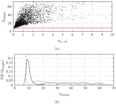
Figure 2: Dependence of noise STD estimates on relative CRLB
σ2
σn·relfor the image 14 from the TID2008 database. (a) Sample STD,
σsample, within a 7×7 SW versusσσn·rel; (b) distribution ofσsamplefor
three cases:σσn·rel≤σσn·rel·max(black curve),σσn·rel >2·σσn·rel·max
(green curve) andσσn·rel>4·σσn·rel·max(blue curve).
STD estimates are expected to follow undesirable non-Gaussian distribution). In our experiments, we set σσn·rel·max=0.25.
The utility of relative CRLB σ2
σn·rel for noise STD
estimation problem is illustrated in Figure 2. Figure 2(a) shows sample STD,σsample, within a 7×7 SW versusσσn·rel
for all nonoverlapping SWs of the test image 14 from TID2008 database (Figure 4(b); for database description see the beginning of Section 3). True noise STD used in our experiment, σn0 = 8.06, is shown as horizontal red line.
It can be observed that sample STD is close to the true value for small σσn·rel increasing fast with σσn·rel. Analysis
of distributions of the sample STD for NI SWs (σσn·rel ≤
σσn·rel·max, black plot inFigure 2(b)) and TI SWs (green and
blue plots inFigure 2(b)corresponds toσσn·rel>2·σσn·rel·max
andσσn·rel> 4·σσn·rel·max, resp.) shows that TI SWs should
not be used for noise STD estimation. On the contrary, the distribution for NI SWs is close to the desirable one: it is centered close to the true value (marked by dashed vertical line) and with significantly shorter right-hand tail.
2.4. ML Estimators for Texture Parameters and Noise STD. To implement the detector (8), the parameter vectorθ is to be estimated for the whole image (for both NI and TI SWs). The goal of the first stage of our algorithm is to estimateθ for SWs that belong to TI map. As TI SWs do not provide information on noise STD, we fix noise STD equal to either an initial guess σn = σn·i=0 or previously estimated value
σn=σn·i−1. Note that in the additive noise case,σnis the same for all SWs. Hereafter, indexidenotes a current iteration of the algorithm. Initial guess for the estimationσn·i=0 can be
obtained as the minimum of sample STD estimates over all image nonoverlapping SWs.
The ML estimator of fBm-model parameters,H andσx, in a single TI SW (SWtype·i−1(t0,s0)=“TI”) is given as
σx·(t0,s0)·i,H(t0,s0)·i,σn=σn
= arg min
σx≥0, 0≤H≤1
[lnL(ΔY;θ)].
(9)
Here SWtype·i−1(t0,s0) is an estimate of informative map
obtained at the previous iteration i − 1. Initially, when i = 0, the entire image is considered to be TI. Thus, for each TI SW we estimate the parameter vector as θTI =
(σx·(t0,s0)·i,H(t0,s0)·i,σn).
Next, the goal of the second stage is to estimateθ for all NI SWs (SWtype·i−1(t0,s0)=“NI”). In this case, we can use
the estimateσn=σn·i−1for noise STD as well. Following the
discussion above, the Hurst exponent,Hpr·(t0,s0)·i, in the NI SWs centered at (t0,s0) is predicted from all current TI SWs
in the neighborhood of pixel (t0,s0) by simple averaging:
Hpr·(t0,s0)·i= 1
|Ω|
(t,s)∈Ω
H(t0,s0)·i, (10)
whereΩ = {(t,s),t /=t0,s /=s0,|t−t0| < Na,|s−s0|< Na, SWtype·i−1(t,s)=“TI”},Nalimits the averaging support. We selectNa =2·Nmeaning that 5×5 nonoverlapping SWs are used. In case |Ω| = 0, we fixHpr·(t0,s0)·i = HTI·mean,
whereHTI·meanis the Hurst exponent estimates average over
all current TI SWs.
It is assumed that the value H describing texture roughness is slowly varying with spatial coordinates (e.g., the sameHvalue can be used to describe a large uniform textural area) and, thus, it can be predicted by (10). On the contrary, σx describing texture amplitude can vary significantly from SW to SW and should be estimated directly from the data as
σx·(t0,s0)·i,H=Hpr·(t0,s0)·i,σn=σn·i−1
=arg min σx≥0
[lnL(ΔY;θ)]. (11)
As a result, for each NI SW we estimate the parameter vector asθNI=(σx·(t0,s0)·i,Hpr·(t0,s0)·i,σn).
At this stage, we haveθ estimated for the whole image. To estimate the CRLBσσ2n·(t0,s0)·i by (7), the value ofσH2 still remains unknown. This value can be estimated from TI map by taking variance of difference between the Hurst exponent estimates obtained by (9) and (10):
σ2 H·i=D
Hpr·(t0,s0)·i−H(t0,s0)·i
, (12)
whereD(·) is the variance operator and variance is calculated over all current TI SWs (SWtype·i−1(t0,s0)=“TI”).
Having vector θ estimated for all NI and TI SWs, we obtain CRLBσ2
σn·(t0,s0)·iin these SWs by substitutingθ =θTI
orθ = θNIandσH2 = σH2·iinto (4) and (7). Finally, we can update discriminative map SWtype·i−1(t0,s0) obtained at the
previous stage to current SWtype·i(t0,s0) map by (8).
to the previously estimated vector θNI. For the updated
SWtype·i(t0,s0) map, we define the ML estimator of noise STD
in a single NI SW (SWtype·i(t0,s0)=“NI”) as
σx·(t0,s0)·i,H=Hpr·(t0,s0)·i,σn·(t0,s0)·i
=arg min σx≥0,σn≥0
[lnL(ΔY;θ)].
(13)
To solve constrained optimization problems (9), (11), and (13), we have used the Han-Powell optimization method described in [32]. This method belongs to the quasi-Newton group and, therefore, it provides high (superlinear) convergence speed which is important for the considered application. In addition, this method includes quadratic programming step for which efficient standard procedures are available.
Finally, we update the current noise STD estimate for the whole image by calculating a weighted average over all current NI SWs:
σn·i=
SWtype·i(t0,s0)=“NI”
σn·(t0,s0)·i/σσ2n·(t0,s0)·i
σ2
σn·NI
,
σ2
σn·NI=
⎛ ⎜
⎝
SWtype·i(t0,s0)=“NI” σ−2
σn·(t0,s0)·i
⎞ ⎟ ⎠ −1
,
(14)
where σ2
σn·NI is estimated CRLB on additive noise STD
estimateσn·ifrom the whole NI map.
For comparison purpose, in addition to the fBm-based estimator (14), let us consider also DCT-based estimator at STD estimation stage of our algorithm. STD estimators based on DCT have demonstrated themselves to be quite accurate for high complexity images [14,33], that is why we expect this approach to perform well within our framework. The additionally proposed estimator performs as follows. For each NI SW, we apply 7×7 DCT and consider only the six highest frequency coefficients with indices (7, 7), (6, 7), (7, 6), (6, 6), (5, 7), and (7, 5). These DCT coefficients are almost insensitive to image content because of two reasons. First, they are calculated for NI SWs. Second, high frequency components of orthogonal transforms are known to be less influenced by image content than low frequency ones [15]. These DCT coefficients are collected from all NI scanning windows (SWtype·i(t0,s0) = “NI”) and the final noise STD
estimate,σn·i, is obtained as sample STD of the formed array of DCT coefficients.
The use of six coefficients allows estimating noise STD in each SW with fixed relative STD 1/√2·6 ≈0.29. This is in agreement with the earlier selected thresholdσσn·rel·max=
0.25.
Before proceeding further, we would like to emphasize the meaning and practical importance of σσ2n·NI value
pro-vided within our scheme. On one hand, it establishes one possible theoretical lower bound on noise STD estimate variance from a given image. On the other hand, it can be estimated directly from a noisy image making it practically interesting since no reference image is needed for deriving
σ2
σn·NI. In the experimental part of the paper, we will provide
|σn·i−1−σn·i|< ε
No
i=i+ 1 Yes
σn
1. Estimate noise STD in each SW belonging to the current noise-informative map using (13)
2. Update global noise STD estimate by (14) or using DCT-based estimator
Noise STD estimation stage 4
1. Update relative CRLB on noise STD in each SW using (7)
2. Discriminate between NI and TI SWs according to the comparison of relative CRLB on noise STD with some predefined threshold using (8)
Update NI/TI decision map 3
Texture parameters estimation stage 2
1. Fix noise STD. Estimate texture parameters by (9) for each SW belonging to current TI map
2. Estimate Hurst exponent for SWs belonging to current NI map using (10)
3. Estimate texture parameters by (11) for each SW belonging to current NI map
Start with TI map as the whole image Initialize global guess for noise STD
Initialization stage 1
Figure3: Generalized scheme of the proposed iterative noise STD estimation algorithm.
some results showing how close to this bound our and two state-of-the-art noise STD estimators (BM3D and SBIQ, see details inSection 3) are.
2.5. Estimator Structure and Convergence. The generalized scheme of the proposed iterative noise STD estimation algorithm is given inFigure 3.
To understand the algorithm convergence, let us consider an extreme case for which noise intensity is negligible with respect to texture intensity in TI areas (local SNR approaches infinity where local SNR is defined as the σ2
NI areas take high and low values with respect to unity, convergence is also reached but with a smaller rate.
3. Accuracy Analysis of Noise STD Estimation
Using TID2008 Database
For analysis purpose, the database TID2008 [34] was chosen (available at http://ponomarenko.info/tid2008.htm). This choice is mainly explained by the following reasons. First, TID2008 comprises 25 color images with low level of self-noise. 24 images are taken from Kodak image database http://r0k.us/graphics/kodak/ and one is artificially synthe-sized (the 25th). All images are of equal size of 512 ×
384 pixels. The database includes images with different content. Some of them have quite large homogeneous areas, the others are quite textural. This allows testing the proposed estimator for images with different content. Second, the database includes images corrupted by additive white Gaussian noise with variance 65, 130, 260, and 520. From practical point of view, the first two cases are of interest. The noisy images with smaller noise variance values can be generated based on practically noise-free reference images provided in the database. Third, the TID2008 database has been used to evaluate performance of several state-of-the-art noise STD estimators [10,14,35]. Thus, the testing results reported previously can be used for comparisons.
In this section, we analyze performance of two versions of the proposed noise STD estimator (later referred to as NI+fBm or NI+DCT depending on which algorithm is used for noise STD estimation from NI map: fBm- or DCT based). Their respective performance is then compared to two state-of-the-art estimators: the BM3D estimator based on nonlocal 3D DCT transform [14] and the segmentation-based interquantile estimator (below it is referred to as SBIQ [35]). Here we would like to thank A. Foi for passing us the results for the BM3D estimator for noise variance equal to 25 and 130.
Color images in TID2008 are represented by 24 bit data arrays, so for each color component the image values are bounded above and below by Imax = 255 and Imin = 0,
respectively. As a result, noisy images in significantly dark or bright areas become clipped. As clipping effect deviates noise distribution from Gaussian and makes its variance smaller, this leads to negatively biased noise STD estimates [36]. To alleviate this effect, we have detected and removed from further consideration SWs affected by clipping effects. This has been carried out using the following rule: a SW is rejected if more than 10% of its pixels have intensity equal toIminor
Imax.
Let us start by presenting examples of NI and TI maps obtained at convergence (4 iterations were needed to obtain these maps). Figures4(a)and4(b)give examples for noisy test images 13 and 14 (σn20 = 65), respectively. Color and
gray tones are associated to NI and TI SWs, respectively. One can see that the NI maps are mainly comprised of HAs (sky inFigure 4(a)and boat surface inFigure 4(b)) and areas with nonintensive texture (nonintensive forest pattern inFigure 4(a)and water surface in Figures4(a)and4(b)). On
the contrary, TI maps include textural areas (intensive forest pattern inFigure 4(a)and intensive water pattern in Figures 4(a)and4(b)) and edges.
The Hurst exponent estimates,Hr·(t0,s0), obtained for the
reference image 13 (considered as noise-free) are displayed as a map inFigure 4(c).Figure 4(d)displays the corresponding
Hpr·(t0,s0)map with areas affected by the clipping effect shown
as black. It can be well observed that Hpr·(t0,s0) map is a
smoothed version of theHr·(t0,s0) map. Similar observations
hold for other images from TID2008 database. These results demonstrate possibility of using (10) forHprediction in NI areas.
The properties of NI map are illustrated inFigure 5for the image 14 andσ2
n0 = 65. First,Figure 5(a)compares the
empirical probability density functions (pdf) of two noise local STD estimates obtained for 7×7 NI SWs. The first pdf is for fBm-based estimatesσx·(t0,s0)given by (13) (shown in
black color). The second pdf relates to sample STD estimates for the six highest DCT frequency coefficients, σDCT·(t0,s0)
(shown in green color). The third pdf corresponds to the standard sample STD (shown in blue color).
As it is seen, the standard sample STD pdf is significantly shifted with respect to the true value of noise STD. This is due to influence of low intensity texture (there are practically no really homogeneous areas in real-life images). Both fBm-and DCT-based estimates are almost unbiased. The only difference is that the fBm-based estimates have notably smaller variance compared to the DCT-based estimates. To highlight this difference,Figure 5(b)shows the correspond-ing empirical pdfs of noise STD estimates normalized by
σx·(t0,s0)−σn0
σσn·(t0,s0)
,
σDCT·(t0,s0)−σn0
σσn·(t0,s0) .
(15)
The normalized estimates can be considered as Gaussian-like distributed random variables with variance close to unity for the fBm-based estimates (theoretical pdfN(0, 1) is shown for comparison as red curve). Estimation variance for DCT-based method is about 2.5 times larger. This difference in estimation accuracy is explained by the fact that the DCT-based estimator uses only six coefficients in each NI SW. Thus, in homogeneous NI SWs, where up to 7·7=49 pixels can be used for noise STD estimation in 7×7 SW, accuracy of the DCT-based estimator is lower than CRLB σσn·(t0,s0).
On the contrary, our fBm-based estimator allows estimating noise STD with accuracy close to CRLBσσn·(t0,s0)in each NI
SW.
As the estimated CRLB value, σσn·(t0,s0), is close to the
actual STD of σx·(t0,s0) estimates in each NI SWs, we can
expect CRLBσσ2n·NI(14) to be a valid estimate of the potential
variance of the global noise STD estimate that can be obtained from NI maps.
One can expect that the accuracy for all methods depends upon image complexity and noise variance. Image complex-ity can be, in particular, characterized by the number of detected NI SWsNNIor, more generally, by the ratioNNI·rel=
NNI/NSW, whereNSWis the total number of nonoverlapping
(a) (b)
0.2 0.4 0.6 0.8 1
(c)
0.2 0.4 0.6 0.8 1
(d) Figure4: NI maps for the test images 13 and 14 (NI SWs are marked by magenta, TI are in gray tones,σ2
n0=65) (a) and (b);Hrmap for the
test image 13, black and white colors corresponds toH=0 andH=1, respectively, (c);Hprmap for noisy image 13,σn20=65 (d).
TID2008 keeping in mind that the larger NNI·rel should
produce better accuracy of noise variance estimation. ValuesNNI·relfor all images of TID2008 database and for
σ2
n0 = 25, 65 and 130 are shown in Figure 6.NNI·rel varies
from 80% for images comprised of large homogeneous areas like (3, 4, or 23) to 1% for the highly textural image 13. This explains why it is difficult to provide high accuracy of blind estimation of noise STD for textural images.
Note that NI map also depends on noise variance. In general,NNI increases withσn20due to reduced influence of
image texture. For example, ifσn20increases from 25 to 130,
NNIon the average increases by 2.2 times (in particular, by
11 times for image 13 and by 1.02 times for the synthetic image 25). As a result, we expect noise variance estimators to be more efficient for largerσ2
n0. This fact is well known in
practice for different estimators [10].
Within the proposed approach, the CRLB σ2 σn·NI can
characterize this tendency quantitatively. Let us consider the relative CRLBσ2
σn·NI·rel = σσ2n·NI/σn20. Under assumption
of Gaussian distribution of noise STD estimates and their unbiasedness, relative CRLB determines potential 99.7% interval forσnasσn∈σn0·[1−3·σσn·NI·rel, 1 + 3·σσn·NI·rel].
The values of σσn·NI·rel obtained for images in TID2008
database are given inFigure 7. It can be observed from this figure thatσσn·NI·rel steadily decreases ifσn20 becomes larger.
For example, withσ2
n0increasing from 25 to 130,σσn·NI·rel, on
the average, reduces by 1.6 times. Averaging above is done for all images of the considered database. Average values of σσn·NI·rel are equal to 0.27% for σn2 = 130 and to 0.45% for σ2
n = 25. This means that for σn20 = 130, noise STD
estimates in the ideal case should belong to a very narrow range 11.4·[1−3·0.0027, 1 + 3·0.0027] ≈ [11.3, 11.5]. Similarly, forσ2
n0 = 25 this interval becomes 5·[1−3·
0.0045, 1 + 3·0.0045]≈[4.93, 5.07].
Let us now test the performance of the NI+fBm, NI+DCT, BM3D, and SBIQ noise STD estimators for all images of the TID2008 database. Initially, our estimator has been applied to all 25 reference images of the TID2008 database in order to estimate noise that originally affects the database images considered almost noise-free. The results of noise STD estimation by NI+DCT for reference images,σr, are consistent for all considered images, varying from 0.3 to 2.
In Figure 8, convergence of NI+DCT estimator for the
red channel of image 14 is shown. The true noise STD is σn0 = 8.06 (σn20 = 65) and it is marked by dashed thin
horizontal line. The black curve corresponds to the situation when initial guessσn·i=0 was selected as described above in
Section 2: the minimal sample STD estimate over all image
nonoverlapping SWs has been used as σn·i=0. In this case,
0 0.1 0.2 0.3 0.4
(
σc
)
5 10 15
σc
(a)
0 0.1 0.2 0.3 0.4 0.5
(
σc
)
−6 −4 −2 0 2 4 6
σc
(b)
Figure5: Distributions (empirical pdfs) of the noise STD estimates for 7×7 NI SWs: (a) pdf ofσx·(t0,s0) estimates (black curve); pdf
of sample STD for the DCT based method (green curve); pdf of standard sample STD (green curve). The true valueσn0is marked as
dashed vertical line; (b) pdf of the normalized noise STD estimates for fBm and DCT-based estimators. True noise STD is marked by dashed vertical line.
Experiments show that our algorithm converges in 3 to 6 iterations in most cases. Texture parameters estimation is the most computationally intensive part as the corresponding parameters need to be estimated for the whole image: the total time cost for 384 by 512 image on Intel Core (TM) 2 Duo (1.66 GHz) CPU varies from 3 to 10 minutes depending on image complexity.
To demonstrate the robustness of the estimator with respect to possible large initial error of noise STD estimation, the same estimator was tested for two other initial guesses:
σn·i=0 =16.0 andσn·i=0 = 4.0. In both cases, the estimator
has converged to the same noise STD final estimate, but it has taken more iterations (six iterations instead of four).
Next, we have considered additive noise case with three different noise STDs:σ2
n0 = 25, 65 and 130. Recall that for
the noisy images for σ2
n0 = 65 and σn20 = 130 are directly
available from the TID2008 database. The noisy images for
0 20 40 60 80 100
100%
NNI
·
re
l
(
k
)
0 5 10 15 20 25
k
Figure6: The number of NI SWs,NNI·relversus image indexkfor
the TID2008 database for noise varianceσ2
n0=25 (blue curve), 65
(red curve) and 130 (black curve).
0 0.5 1 1.5 2 2.5
100%
σNI
·
re
l
(
k
)
0 5 10 15 20 25
k
Figure 7: Noise STD estimation accuracyσσn·NI·rel versus image
indexk for the TID2008 database for noise varianceσ2
n0 equal to
25 (blue curve), 65 (red curve), and 130 (black curve).
4 6 8 10 12 14 16
σc
(
i
)
1 2 3 4 5 6
i
Figure 8: Convergence of NI+DCT noise STD estimator. Initial guess for noise STDσn·i=0≈7.0 (black curve),σn·i=0 =16.0 (blue
curve) andσn·i=0=4.0 (red curve).
σn20 = 25 have been generated by adding synthetic noise
with the corresponding variance followed by quantization and clipping to the range from 0 to 255. As the obtained noisy images contain both the reference images noise and the synthetic noise subsequently added, the resulting noise STD is slightly larger thanσn0. Therefore, the estimates for all
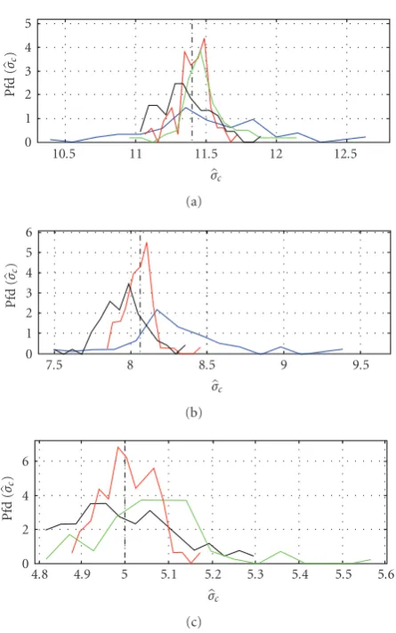
considered methods have been corrected asσc=
σ2−σ2
r. The empirical pdfs of the obtained estimates are pre-sented inFigure 9for three noise variances for the proposed NI+fBm and NI+DCT estimators (in black and red colors, resp.), the BM3D estimator (in green color) and SBIQ esti-mator (in blue color). The corresponding mean (Mean(σc)) and STD (STD(σc)) of the obtained estimates over the whole TID2008 database are given inTable 1.
Table1: Mean and STD of additive noise STD estimatesσcfor TID2008 database.
Mean(σc)/STD(σc) σn20=25 (σn0=5) σn20=65 (σn0=8.06) σn20=130 (σn0=11.40)
NI+fBm 5.00/0.120 7.96/0.156 11.35/0.183
NI+DCT 5.01/0.060 8.05/0.098 11.41/0.121
BM3D 5.06/0.128 —no data available— 11.50/0.196
SBIQ —no data available— 8.29/1.372 11.29/1.59
0 1 2 3 4 5
Pfd
(
σc
)
10.5 11 11.5 12 12.5
σc
(a)
0 1 2 3 4 5 6
Pfd
(
σc
)
7.5 8 8.5 9 9.5
σc
(b)
0 2 4 6
Pfd
(
σc
)
4.8 4.9 5 5.1 5.2 5.3 5.4 5.5 5.6
σc
(c)
Figure9: Empirical pdfs of STD estimatesσcobtained for the whole
TID2008 database by (1) NI+fBm (in black color); (2) NI+DCT (in red color); (3) BM3D (in green color); (4) SBIQ (in blue color); noise variances are equal toσ2
n0=130 (a),σn20=65 (b), andσn20=25
(c). The true noise STD is marked by dashed vertical line in all plots.
According toTable 1, for the SBIQ estimator the STD (σc) takes the largest value ≈1.3–1.5 and Mean(σc) is biased by about 5% (forσn20=65). The BM3D and NI+fBm estimators
show similar performance, reducing STD(σc) by about 5– 8 times compared to SBIQ. Mean(σc) is biased by only ≈1%. The NI+DCT estimator improves these results even further. STD(σc) reduces by about 1.5–2 times as compared to its value for BM3D and NI+fBm; mean(σc) bias becomes negligible (<0.4%). Note that for the NI+DCT estimator the actual ranges ofσc variation are only approximately 2 times
0 0.05 0.1 0.15
Pfd
(
σnor
m
)
−25 −20 −15 −10 −5 0 5 10 15 20 25
σnorm
Figure 10: The empirical pdfs of the normalized noise STD estimatesσnorm. Color settings are as inFigure 9.
wider than the ones determined by CRLB ([11.3, 11.5] for σ2
n0=130 and [4.93, 5.07] forσn20=25). Thus, very accurate
estimation is provided for all images of the considered database irrespectively to noise STD value.
Potentially the method NI+fBm is expected to out-perform NI+DCT estimator (see Figure 5). However, the simulation results have not shown this. The reason seems to be the following. Within the NI+fBm approach, both noise STD and Hurst exponent are estimated jointly with mutual influence on each other. Then, the errors in Hurst exponent prediction lead to additional errors of STD esti-mation, which, consequently, results in accuracy reduction of NI+fBm technique. On the contrary, within NI+DCT approach the Hurst exponent estimates are used only at NI map forming stage, and they do not directly influence the STD estimation stage.
Availability of CRLBσ2
σn·NI allows presenting noise STD
estimated in the normalized form as
σnorm=
(σc−σn0)
σσn·NI
. (16)
Considering σ2
σn·NI as potential noise STD estimation
accuracy, σnorm for an efficient unbiased estimator should
approach normal distribution with zero mean and unit vari-ance. Then, it becomes possible to compare the considered estimators to the efficient one.
Figure 10 presents four empirical pdfs of σnorm for the
NI+fBm and NI+DCT, BM3D and SBIQ estimators (color settings are as inFigure 9). These pdfs have been obtained for all images and all analyzed noise variances. It is seen that the pdf ofσnormfor NI+DCT estimator follows Gaussian-like
distribution with the mean equal to 0.22 and STD equal to 3.16. The pdf ofσnorm for the BM3D (NI+fBm) estimator
2.30 (−2.60) and STD equal to 5.31 (6.29). The empirical pdf for the SBIQ method is also nonsymmetrical one with heavy right and left tails. Its mean equals to −2.24 and its STD is 39.25 (taking into account the outliers mentioned above).
We see that accuracy of all considered estimators is quite far fromσ2
σn·NI. Their statistical efficiency with respect to this
bound can be expressed as
e=100%·NeNe i=1σnorm2 ·i
, (17)
where the sum for each estimator is calculated over all Ne available estimates. For the proposed estimators, we obtain eNI DCT = 10.01% and eNI fBm = 2.17%. One haseBM3D =
3.00% for the BM3D estimator and eSBIQ = 0.07% for
the SBIQ. These results show that the proposed NI+DCT estimator is by 3 times more efficient that the state-of-the-art BM3D estimator, although performance of STD estimators can be further improved considerably. Thus, there is a room for further improvement and research in the area of noise STD blind estimation.
4. Conclusion
In this paper, a novel approach to image noise STD estimation has been proposed. It is mainly based on iterative separation of the processed image into two areas: noise-informative one that is able to provide information on noise STD and texture-informative area that allows estimating texture correlation structure or roughness. The 2D fBm model has been used as the model for image texture.
Such separation provides several advantages. First, it allows solving two complementary problems: to obtain accurate texture parameters for noisy part of the image and accurate noise parameters for textural part of the image, thus making both texture and noise parameters available for the whole image. Second, using texture and noise parameters, the Fisher information that a single SW contains about noise STD (or CRLBσ2
σn on noise STD estimates) has been determined to refine current NI and TI maps.
The experiments on TID2008 database have shown that separation on NI and TI maps can be successfully carried out for real-life images. NI maps for these images may occupy from 1 to 80% of image area depending on their homogeneity. The relative area of the NI map increases with noise variance.
Availability of CRLB σ2
σn allows determining potential variance of additive noise STD estimation from the whole NI map. We have used this bound to compare the efficiency of our estimators to that of two state-of-the-art estimators: BM3D and SBIQ method. We found NI+DCT estimator to significantly outperform the BM3D and SBIQ estimators. At the same time, the designed NI+DCT estimator provides noise STD estimates with STD approximately 3 times larger than the estimated potential STDσσn·NI. Thus, the design of
more efficient noise STD estimator is challenging.
References
[1] M. Elad,Sparse and Redundant Representations. From Theory to Applications in Signal and Image Processing, Springer Science + Business Media, LLC, 2010.
[2] B. Vozel, S. K. Abramov, and K. Chehdi, “Blind determination of noise type for spaceborne and airborne remote sensing,” in
Multivariate Image Processing, C. Collet, J. Chanussot, and K. Chehdi, Eds., chapter 9, p. 464, Wiley-ISTE, 2009.
[3] F. D. Van Der Meer and S. M. Dejong,Imaging Spectrometry: Basic Principles and Prospective Applications, Kluwer Academic Publishers, Dodrecht, The Netherlands, 2001.
[4] S. Gao and T. D. Bui, “Image segmentation and selective smoothing by using Mumford-Shah model,” IEEE Transac-tions on Image Processing, vol. 14, no. 10, pp. 1537–1549, 2005. [5] A. de Santis and D. Iacoviello, “A region growing method for medical images segmentation,” International Journal of Tomography and Statistics, vol. 13, no. 10, pp. 19–37, 2010. [6] V. V. Lukin, S. K. Abramov, N. N. Ponomarenko et al.,
“Processing of images based on blind evaluation of noise type and characteristics,” inImage and Signal Processing for Remote Sensing, vol. 7477 ofProceedings of SPIE, p. 12, Berlin, Germany, 2009.
[7] P. Chatterjee and P. Milanfar, “Fundamental limits of image denoising: are we there yet?” inProceedings of the IEEE Inter-national Conference on Acoustics, Speech and Signal Processing (ICASSP ’10), pp. 1358–1361, Dallas, Tex, USA, 2010. [8] K. Dabov, A. Foi, V. Katkovnik, and K. Egiazarian, “Image
denoising by sparse 3-D transform-domain collaborative filtering,”IEEE Transactions on Image Processing, vol. 16, no. 8, pp. 2080–2095, 2007.
[9] B. Aiazzi, L. Alparone, A. Barducci et al., “Noise modelling and estimation of hyperspectral data from airborne imaging spectrometers,”Annals of Geophysics, vol. 49, no. 1, pp. 1–9, 2006.
[10] V. Lukin, S. Abramov, M. Uss et al., “Testing of meth-ods for blind estimation of noise variance on large image database,” inTheoretical and Practical Aspects of Digital Signal Processing in Informational-Telecommunication Systems, V. I. Marchuk, Ed., South-Russian State University of Economics and service, Shakhty, Russia, 2009, http://k504.xai.edu.ua/ html/prepods/lukin/BookCh1.pdf.
[11] B. C. Gao, “An operational method for estimating signal to noise ratios from data acquired with imaging spectrometers,”
Remote Sensing of Environment, vol. 43, no. 1, pp. 23–33, 1993. [12] R. E. Roger and J. F. Arnold, “Reliably estimating the noise in AVIRIS hyperspectral images,”International Journal of Remote Sensing, vol. 17, no. 10, pp. 1951–1962, 1996.
[13] N. N. Ponomarenko, V. V. Lukin, M. S. Zriakhov, A. Kaarna, and J. Astola, “An automatic approach to lossy compression of AVIRIS images,” inProceedings of the International Geoscience and Remote Sensing Symposium (IGARSS), pp. 472–475, Barcelona, Spain, 2008.
[14] A. Danielyan and A. Foi, “Noise variance estimation in non-local transform domain,” inProceedings of the International Workshop on Local and Non-Local Approximation in Image Processing (LNLA ’09), pp. 41–45, August 2009.
[15] L. S¸endur and I. W. Selesnick, “Bivariate shrinkage with local variance estimation,”IEEE Signal Processing Letters, vol. 9, no. 12, pp. 438–441, 2002.
[16] A. De Stefano, P. R. White, and W. B. Collis, “Training meth-ods for image noise level estimation on wavelet components,”
[17] J. S. Lee and K. Hoppel, “Noise modeling and estimation of remotely-sensed images,” Proceedings of the International Geoscience and Remote Sensing Symposium (IGARSS ’89), vol. 2, pp. 1005–1008, 1989.
[18] L. Alparone, M. Selva, L. Capobianco, S. Moretti, L. Chiaran-tini, and F. Butera, “Quality assessment of data products from a new generation airborne imaging spectrometer,” in
Proceedings of the IEEE International Geoscience and Remote Sensing Symposium (IGARSS ’09), vol. 4, pp. IV422–IV425, July 2009.
[19] V. V. Lukin, S. K. Abramov, A. A. Zelensky, J. T. Astola, B. Vozel, and K. Chehdi, “Improved minimal inter-quantile distance method for blind estimation of noise variance in images,” inImage and Signal Processing for Remote Sensing, vol. 6748 ofProceedings of SPIE, p. 12, Florence, Italy, 2007. [20] V. V. Lukin, S. K. Abramov, B. Vozel, and K. Chehdi, “A
method for blind automatic evaluation of noise variance in images based on bootstrap and myriad operations,” in
Image and Signal Processing for Remote Sensing, vol. 5982 of
Proceedings of SPIE, pp. 299–310, Bruges, Belgium, 2005. [21] C. Liu, R. Szeliski, S. B. Kang, C. L. Zitnick, and W. T. Freeman,
“Automatic estimation and removal of noise from a single image,”IEEE Transactions on Pattern Analysis and Machine Intelligence, vol. 30, no. 2, pp. 299–314, 2008.
[22] B. Xu and P. Gong, “Noise estimation in a noise-adjusted principal component transformation and hyperspectral image restoration,”Canadian Journal of Remote Sensing, vol. 34, no. 3, pp. 271–286, 2008.
[23] L. Klaine, B. Vozel, and K. Chehdi, “Unsupervised variational classification through image multi-thresholding,” in Proceed-ings of the 13th EUSIPCO Conference, p. 4, Antalya, Turkey, 2005.
[24] M. Wettle, V. E. Brando, and A. G. Dekker, “A methodology for retrieval of environmental noise equivalent spectra applied to four Hyperion scenes of the same tropical coral reef,”Remote Sensing of Environment, vol. 93, no. 1-2, pp. 188–197, 2004. [25] S. K. Abramov, V. V. Lukin, B. Vozel, K. Chehdi, and J. T.
Astola, “Segmentation-based method for blind evaluation of noise variance in images,” SPIE Journal of Applied Remote Sensing, vol. 2, no. 1, p. 15, 2008.
[26] L. R. Gao, B. Zhang, X. Zhang, W. J. Zhang, and Q. X. Tong, “A new operational method for estimating noise in hyperspectral images,”IEEE Geoscience and Remote Sensing Letters, vol. 5, no. 1, pp. 83–87, 2008.
[27] C. Kervrann and J. Boulanger, “Local adaptivity to variable smoothness for exemplar-based image regularization and representation,”International Journal of Computer Vision, vol. 79, no. 1, pp. 45–69, 2008.
[28] W. Sun, G. Xu, P. Gong, and S. Liang, “Fractal analysis of remotely sensed images: a review of methods and applica-tions,”International Journal of Remote Sensing, vol. 27, no. 22, pp. 4963–4990, 2006.
[29] B. Pesquet-Popescu and J. L. V´ehel, “Stochastic fractal models for image processing,”IEEE Signal Processing Magazine, vol. 19, no. 5, pp. 48–62, 2002.
[30] B. B. Mandelbrot and J. W. Van Ness, “Fractional brownian motions, fractional noises and applications,”SIAM Review, vol. 10, no. 4, pp. 422–437, 1968.
[31] K. Falconer,Fractal Geometry: Mathematical Foundations and Applications, John Wiley & Sons, 2003.
[32] D. G. Luenberger, Linear and Nonlinear Programming, Addison-Wesley, Reading, Mass, USA, 2nd edition, 1984.
[33] N. N. Ponomarenko, V. V. Lukin, M. S. Zriakhov, A. Kaarna, and J. Astola, “An automatic approach to lossy compression of AVIRIS images,” inProceedings of the International Geoscience and Remote Sensing Symposium (IGARSS ’08), pp. 472–475, Barcelona, Spain, 2008.
[34] N. Ponomarenko, V. Lukin, K. Egiazarian, J. Astola, M. Carli, and F. Battisti, “Color image database for evaluation of image quality metrics,” in Proceedings of the IEEE 10th Workshop on Multimedia Signal Processing (MMSP ’08), pp. 403–408, October 2008.
[35] V. Lukin, S. Abramov, M. Uss, B. Vozel, and K. Chehdi, “Performance analysis of segmentation-based method for blind evaluation of additive noise in images,” inProceedings of MSMW, p. 3, Kharkov, Ukraine, 2010.