Real-time Linux
in Control Applications Area
R.A. Stephan
M.Sc.Thesis
Supervisors: prof.dr.ir. J. van Amerongen
dr.ir. J.F. Broenink
ir. D. Jovanovic
ir. G.H. Hilderink
Faculty of
Electrical Engineering
University of Twente
August 2002 Report Number 016CE2002
Control Engineering Faculty of Electrical Engineering
University of Twente P.O. Box 217
Summary
This thesis describes the design and realization of control software and drivers for a mechatronic setup. The mechatronic setup has two degrees of freedom, and a separate controller controls each joint. The software design and implementation is done according to Communicating Sequential Processes (CSP) concepts on a real-time Linux (RTLinux) platform.
Real-time Linux is a hard real-time version of the standard Linux. It has the facilities the timing requirements needed to provide real-time behaviour. All the functionality of the normal Linux is available for development.
Communicating Threads for C++(CTCPP) (Hilderink, 2001) is an object oriented software package developed at Control Engineering. This package provides a clear way of concurrent programming based on the theory of Communicating Sequential Processes (CSP). With CSP a concurrent system can be described by concurrently running processes that communicate with each other via channels.
The C++ code for the two controllers is generated with the 20-sim program.
A set of device drivers has been developed for the used fast professional data acquisition board. This has been done in the C++ programming language. Test utilities for testing the drivers have been created. FIFO communication and data logging have been implemented. A console line print routine to print to screen from a real-time process has also been created.
Some performance aspects of RTLinux and CSP have been analysed by means of two test programs. The interrupt latency of RTLinux and the channel communication time of CSP under RTLinux have been measured. The CSP package has a maximum channel communication time of 5.06 µs. The interrupt latency of RTLinux is at most 8 µs.
The setup dependent parts have been implemented. The two controllers needed to drive the setup have been generated with 20-sim. A design for a controller with CSP has been given. This controller will use interrupt clocked IO to minimize the hardware delays. The performance of the controller was measured. The X-axis has a maximum error of 4 % and the Y-axis has a maximum error of 6.6 %.The steady state errors are 0.38 % and 0.12 % respectively.
Samenvatting
Dit verslag beschrijft het ontwerp en de implementatie van een mechatronische opstelling met twee vrijheidsgraden. Elke as wordt door een aparte controller bestuurd. dat door een controller,
geïmplementeerd met Communicating Sequential Processes (CSP) concepten, draaiend op real-time Linux (RTLinux).
Real-time Linux is een hard real-time versie van de standaard Linux. RTLinux kan de tijdslimieten halen die nodig zijn voor hard real-time gedrag. Alle functionaliteit van de standaard Linux is beschikbaar voor ontwikkeling.
Communicating Threads for C++ (CTC++) is een object georiënteerd software pakket dat door Control Engineering is ontwikkeld. Het pakket levert een manier van parallel programmeren gebaseerd op de theorie van Communicating Sequential Processes (CSP). Met CSP kan een parallel systeem beschreven worden door middel van parallel draaiende processen die met elkaar
communiceren over kanalen.
De C++ code voor de controller is gegenereerd door het pakket 20-Sim.
Een set device drivers voor de gebruikte snelle data acquisitie kaart is ontwikkeld in de C++ programmeer taal. Test programma’s voor de verschillende modules op de IO kaart zijn gemaakt. FIFO communicatie en data logging zijn geïmplementeerd. Een programma om tekst van uit een real-time proces op het scherm te printen is ook gemaakt.
Bepaalde prestaties van RTLinux en CSP zijn gemeten en geanalyseerd met twee test programma’s. De interrupt vertraging van RTLinux en de kanaal communicatie tijd van CSP onder RTLinux zijn gemeten. Het CSP pakket had een kanaal communicatie tijd van maximaal 5.06 µs. De interrupt vertraging van RTLinux is op zijn hoogst 8 µs.
De opstelling afhankelijke delen zijn geïmplementeerd. De twee controllers die nodig zijn om de opstelling aan te sturen is gegenereerd met 20-sim.Een ontwerp voor een controller met CSP is gegeven. Deze controller zal gebruik maken van interrupt gestuurde IO om de hardware vertraging te minimaliseren De prestaties van de controllers zijn gemeten. De maximale fout in de X-as is 4 % en de maximale fout in de Y-as is 6.6 %. De stationaire fouten zijn respectievelijk 0.38 % en 012 %.
Acknowledgements
Although in the beginning I had no idea what I was getting in to, it has been a very interesting project. I had to (re)master several subjects with which I was not too familiar. Now, at the end of the project, the subjects are familiar but new ideas and concepts are waiting to be explored.
I would like to thank my supervisors who gave me the opportunity to work on this very promising and interesting subject.
Job van Amerongen I would like to thank for the opportunity to graduate at the Control Laboratory.
Jan Broenink I thank for giving me a direction to go when I had no idea what subject to explore during my Master of Science project.
My supervisors Dusko and Gerald I want to thank for the enthusiasm with which they both took up the task of guiding Peter and me. Also the weekly meetings with you were both fun and helpful, not in the least for the practice in English and the vitamins in the fruit.
All the students at the lab thanks for the fun we had, when we actually should have been working…
Especially I want to thank my family for supporting me all these years.
Contents
1 INTRODUCTION... 1
1.1 OBJECTIVES... 1
1.2 REAL-TIME AND CONCURRENT PROGRAMMING... 1
1.3 THE DESIGN TRAJECTORY AND ITS HISTORY... 2
1.3.1 The early THESIS approach ... 2
1.3.2 Changes in the design methodology ... 3
1.4 CURRENT METHODOLOGY... 4
1.5 OUTLINE OF THE REPORT... 4
2 DEVELOPMENT ENVIRONMENT... 5
2.1 REAL-TIME LINUX... 5
2.1.1 Scheduling... 6
2.1.2 Interrupts ... 7
2.2 COMMUNICATING THREADS FOR C++ ... 7
2.2.1 Producer – Consumer Example... 8
2.3 20-SIM... 10
2.4 SETUP IOINTERFACE... 11
2.5 REVIEW... 12
3 SOFTWARE DEVELOPMENT... 13
3.1 DATA ACQUISITION BOARD DEVICE DRIVERS... 13
3.1.1 System Timing and Control Module ... 14
3.1.2 Analog Output Timing Module ... 15
3.1.3 Analog Input Timing Module... 16
3.1.4 Digital IO Module... 16
3.1.5 Counter / Timer Module ... 17
3.1.6 Programmable Function Inputs Module... 17
3.1.7 Miscellaneous Functions ... 17
3.2 SUPPORT UTILITIES... 18
3.2.1 Test Utilities... 18
3.2.2 RT-FIFO ... 18
3.2.3 Console ... 19
3.2.4 Logger... 20
3.3 SYSTEM TEST PROGRAMS... 22
3.3.1 Comstime ... 22
3.3.2 Interrupt Latency ... 24
3.4 REVIEW... 25
4 CASE STUDY: JIWY... 27
4.1 CONTROLLER INPUT... 27
4.1.1 The Joystick ... 27
4.1.2 Digital Filter... 28
4.2 PLANT DESCRIPTION... 28
4.2.1 JIWY... 28
4.2.2 Bondgraph model... 29
4.2.3 The Box ... 30
4.3 CONTROL SOFTWARE IMPLEMENTATION... 30
4.3.1 Controller simulation models ... 31
4.3.2 Controller Generation models ... 31
4.3.3 Controller with CSP ... 32
4.4 CONTROLLER PERFORMANCE... 33
5 CONCLUSIONS & RECOMMENDATIONS ... 37
5.1 CONCLUSIONS... 37
5.2 RECOMMENDATIONS... 37
A. INFORMATION AND LINKS ... 39
LINUX... 39
RTLINUX... 39
CPPDOC... 39
CAMSTREAM... 39
B. DIRECTORY STRUCTURES ... 40
CT PACKAGE STRUCTURE... 40
PROJECT STRUCTURES... 41
COMPILE SCRIPT... 42
C. HARDWARE DECISION LIST ... 43
D. PLANT DETAILS ... 44
WIRING... 44
JIWYMOTORS... 45
E. NON CLASS METHODS AND DEFINITIONS ... 46
NI6024E.H... 46
RTL_CONSOLE.C... 47
F. IMPLEMENTATION DETAILS... 48
1 Introduction
At Control Engineering of the department of Electrical Engineering at the University of Twente, great effort is put into developing structured methods for designing real-time systems. To reduce
development time and costs and to prevent errors in the realization of control systems, research has been performed on adequate design methodologies. This resulted in a structured development methodology for embedded real-time control systems, which was called Twente Hierarchical Embedded Systems Implementation by Simulatio (THESIS), (Wijbrans et al., 1993). The objective of the THESIS project is the automated development of reliable and safe control systems in minimum development time.
Real-time (control) systems are parallel by nature. This theorem is obvious as control systems
typically consist of (multiple) sensors and actuators that operate simultaneously. The processing of the sensor data and calculation of the actuator values has to be done at the same time. Often a control problem can be divided into smaller parts, which could be executed in parallel. By using the
Communicating Sequential Processes (CSP) (Hoare, 1978) formalism, a more natural approach and understanding of the control problem and design can be achieved.
For the realization of parallel real-time control systems a computing platform and/or a programming language with support for parallelism and communication is required. In the early stages of THESIS, a combination of the transputerand the Occam programming language was chosen for the target hardware and software. This control environment has become obsolete since development in transputers has stopped and modern microprocessors outperform transputers. Nowadays PCs and Real-Time Linux (RTLinux) are more often used since they provide a relative cheap solution. Therefore this assignment focuses on the use of a standard PC in combination with RTLinux and a CSP.
In order to realize the demo first a PC with Linux and RTLinux was needed. The used PC is a Pentium Pro 200 MHz running Linux Slackware 8.0 with real-time Linux 3.1. Slackware was chosen since at that time it was the only distribution that used the 2.2.19 Linux kernel that was needed for RTLinux 3.1 and higher. To connect the PC to the setup an IO board was needed. An IO board from National Instruments was selected from a number of IO boards.
1.1 Objectives
The aim of this research is to develop a software controller running on the PC using the real-time Linux platform that is controlling a mechatronic setup.
The CSP library will be used to develop the concurrent software. The connection between the PC and the actual setup must be realised using a data acquisition IO board. Device drivers for the data acquisition IO board under RTLinux must be created. Electronics between the IO board and the setup has to be realised to drive the sensors and actuators on the setup. The working system should be demonstrated.
1.2 Real-time and Concurrent Programming
There are several definitions of real-time systems, most of them slightly different. Unfortunately the topic is controversial, and there does not seem to be an exact agreement over the terminology. One could consider the Windows operating system to be real-time. “Real-time” is an over-used term that can be used to mean “right away” or “fast” as in “real-time stock quotes”. In this thesis hard real-time systems are addressed: those with timing deadlines that must not be missed otherwise the system fails.
readability and reusability of code. Also a concurrent methodology is preferable, to allow to execute the tasks in parallel. It does not necessarily mean that these tasks run on distinct hardware because they may also be scheduled one at the time on a single processor. Writing concurrent or parallel software has always been viewed as a minor activity (Gorton et al., 1995). Most software applications do not need to incorporate explicit parallel activities since adequate performance can be achieved by sequential code executing. Real-time control and embedded systems programming however utilize parallelism to achieve additional performance to meet hard real-time constraints. Reasons for using concurrent programming may be:
• A performance gain from (distributed) multi processor hardware or better processor utilisation; • Increased application responsiveness;
• A more appropriate structure; • A faster throughput of data.
1.3 The Design Trajectory and its history
In this section the history of the design trajectory is given. The THESIS design methodology is discussed followed by the changes in hardware, software and specification methods, which made the THESIS approach outdated.
1.3.1 The early THESIS approach
The development of real-time systems, with implementation choices such as hardware interfaces, control algorithms and control software, could become a rather complex process. This is because all these components have influence on the dynamic behaviour of the system. THESIS is a structured methodology in which the dynamic properties of a system play an important role. The main idea of the THESIS project is to develop a system, which covers the complete design trajectory, from obtaining design requirements to generating code, for embedded real-time control systems. An objective of THESIS is the mechatronic design approach. In this approach system development is no longer done by separately developing parts that are integrated later, but the system is treated as a whole. A second objective of THESIS is verification and validation by gradual refinement of the model. The result is a functional description of the model. A third objective is the separate
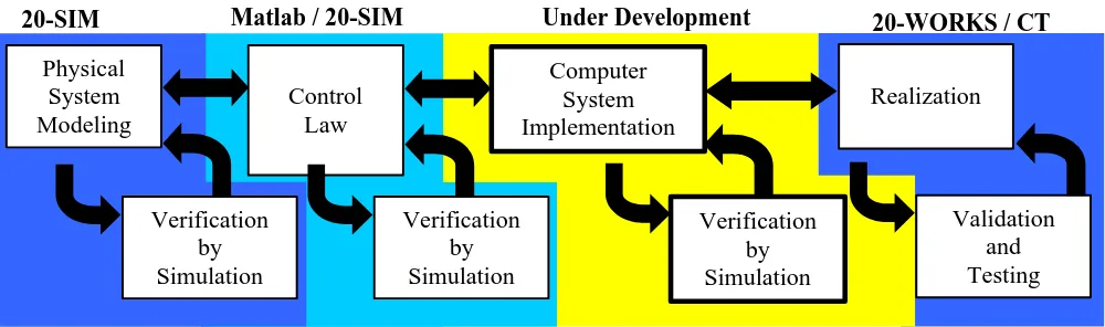
development of parts. These parts (building blocks) are integrated in a later stage. Figure 1 shows the THESIS design trajectory, which includes:
• Physical system modelling: The dynamic behaviour of the system is object-oriented modelled. The 20-Sim software (Broenink, 1997) is a modelling and simulation package used to obtain a correct model;
• Control law design: Using the model acquired in the previous step, a control law or a simplified version of it is designed. External software like Matlab was used, but nowadays mainly 20-sim is used.
• Computer system implementation: the transformation process to convert the control laws (i.e. mathematical formulas) to efficient concurrent algorithms (i.e. computer code) is guided via a stepwise refinement procedure. After each refinement step, the results are verified by simulation. This refinement procedure is prototyped in Wijbrans et al. (1993);
Figure 1: THESIS design trajectory
The part of Figure 1 that states under development is currently being researched. This is done in project TES5224 (Jovanovic, 2001), (Orlic, 2002).
Several implementations of the realization phase have been developed for various target architectures. These implementations form a modular approach to the design and implementation of control
systems, as applied in mechatronic research. The implementations are:
• The RoViCoM (Robot Vision Control Manager) system (Bruis et al., 1993), its target architecture is transputer based;
• 20-Works, for single-processor controlled set-ups, accepting C++ code for the control algorithm (Elgersma, 2000), (Weustink, 1995, 1996);
• The JavaPP (Java Plug ’n Play) project (Hilderink, 2000).
1.3.2 Changes in the design methodology
Due to further developments, the original target software environment is replaced. The usage of modern programming languages to design software based on the CSP concepts has been investigated. The JavaPP (Java Plug ’n Play) is an international collaborative effort that introduces the CSP/occam model into Java (Hilderink, 2000a). The project resulted in similar packages for the programming languages C and C++. Currently, the following packages are available: for Java the Communicating Threads for Java (CTJ) package (Hilderink et al., 2000) and the Java Communicating Sequential Processes (JCSP) (Welch, 1998; Welch and Austin, 2000); for C the Communicating Threads for C (CTC) package (Hilderink, 2000b) and the CCSP package (Moores, 1999) and for C++ the
Communicating Threads for C++ (CTCPP) package (Hilderink, 2000b).
In addition to the modernized target software environment, also the target hardware environment was modernized. The original hardware environment that was supported by THESIS has become obsolete since the development in Transputers has stopped and modern microprocessors outperform the Transputers. In the new control environment, Transputers are replaced by a heterogeneous mixture of microcontrollers / DSPs and the transputer links (OS-links) are substituted by IEEE-1355 Data-Strobe links (DS-links) or other connections (Greve, 1998; Lahpor, 1998).
In addition to the changes in the target hardware and target software also the originally used Ward and Mellor (Ward and Mellor, 1986; Hatley and Pirbhai, 1988) design specification method has become obsolete. Nowadays software design tools like UML are available
There is a fundamental change in the paradigm used by the software industry. The focus is shifted from the tradition system specification and construction, called the waterfall cycle methodology, to one requiring simultaneous consideration of the system context (i.e. system characteristics such as requirements, costs), capabilities of products in the market place, and viable architectures and designs, also called component-based software engineering (CBSE) (Hissam, 2000). In the CBSE
methodology the developer can use existing Components Of The Shell (COTS).
20-WORKS / CT Matlab / 20-SIM
1.4 Current methodology
Nowadays it is impossible to separate control engineering from software engineering: the only efficient way to implement controllers is to transform them into computer code for the chosen target. In control engineering practice, used software development techniques suffer from insufficiencies in knowledge in disciplines of software modelling, familiarity with concurrency in software, ways of allowing for reusability, software testing and so forth. The resulting code functions correctly in first instance, but is generally not reliable in a non-ideal environment, neither efficient nor extendable. The control-computer systems are embedded control systems, because the control computer code is specific to the control system, for which the dynamic behaviour of the setup is essential for the functionality.
Current research deals with the development of a design framework and a supporting software tool to efficiently support the mechatronic engineer in developing sophisticated control computer code out of a set of control laws. Normally, mechatronic design engineers start with modelling the dynamic behaviour of the plant, and derive a control law for it. This control law is then gradually transformed via Stepwise Refinement towards efficient concurrent algorithms (i.e. the control computer code). During this process, simulation is often used as a means of verification. In the end phase, realization can also be done stepwise, namely by letting parts of the total system stay simulated, and letting other parts be in the final realization (Broenink, 2001). Especially the step from control law design to implementation is recognized as critical and not methodologically covered by existing approaches and tools.
For the modelling control law design parts including their simulations, existing tools (20-sim, Matlab) suffice. Often graphical modelling languages, e.g. block diagrams, are used in this design process for structuring and managing the complexity of the control structures. The software development step can conceptually be covered using the CSP parallel processing paradigm. Since tools for modelling and control law design nowadays are graphically oriented, a CSP extension as graphical block diagrams are developed, resulting in CSP diagrams (Hilderink, 2002). CSP diagrams specify concurrency in block diagrams of communicating processes.
1.5 Outline of the Report
2 Development Environment
In this chapter the development environment is discussed. In this project the development
environment is used to develop the software and hardware needed to implement the total system. The environment is made up of several software and hardware tools.
The software tools are the following parts.
• Real-time Linux operating system, which can facilitate the timing requirements for real-time tasks. Real-time Linux can also be used during the software development, because software editors are present on the system.
• The C++ implementation of Communicating Sequential Processes. This package enables the rapid development of reliable real-time concurrent software.
• The 20-sim modeling and simulation package. In 20-sim a model of a physical system can be simulated and a suitable controller for the model can be designed. The latest versions of 20-sim can generate code from models or sub-models, which can be tested in the real world.
The hardware part in the development environment is the selected IO board. The IO board is used to connect the controller running on the PC to the real physical system.
2.1 Real-Time Linux
Real-Time Linux (RTLinux) could be a useful operating system to control a mechatronic setup from a PC. Since it is free and open source, the operating system can be tailored to specific needs. Further all the advantages of the Linux development environment, like X-windows and the network support, are available. While Linux is not capable of guaranteeing the predictable time limits needed for real-time tasks, RTLinux is. The problem with Linux is that Linux, like other general-purpose operating systems, is designed to optimise average performance. This means that all processes will get a fair share of CPU time. For real-time programming precise timing and predictable timing is more
important than average performance. This problem was recognized and research on turning Linux into a hard real-time operating system was started. At FSMlabs (FSMlabs, 2002) this research resulted in Real-Time Linux (RTLinux).
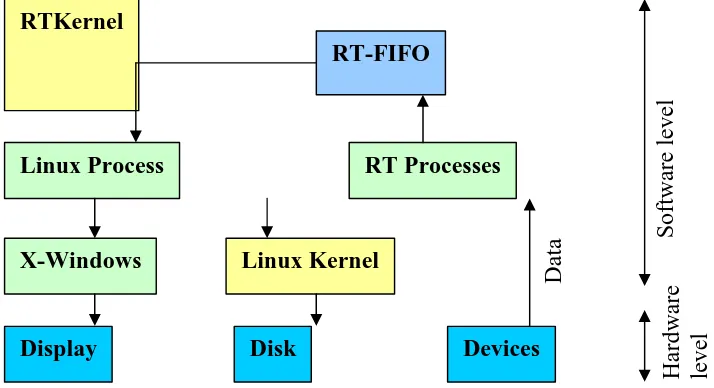
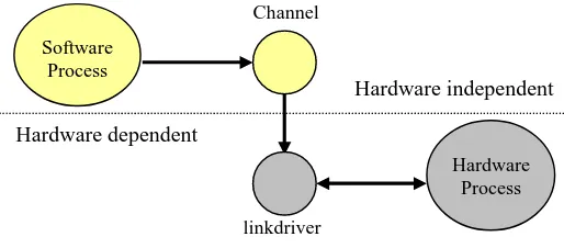
In Figure 2 a data collection application is depicted. The real-time process reads data from a device and transmits the data through a RT-FIFO to a Linux process. The Linux process will show the data on the display and stored on the disk.
Figure 2: Data Collection Application
2.1.1 Scheduling
The RTLinux kernel schedules all the kernel level tasks in a predictable way. When no real-time tasks are scheduled, the RTLinux kernel will schedule the Linux kernel. The Linux kernel schedules all the Linux processes in the standard non-predictable way. A graphical example is shown in Figure 3.
Figure 3: Scheduling Example
The real-time task 1 is scheduled twice as often as real-time task 2. When one of the real-time tasks runs the system will stop the Linux task. If two real-time tasks are running at the same time the task with the highest priority will be executed first. The priority of each task can be set during the thread creation. When no real-time task is running the Linux kernel is scheduled and it will schedule the Linux processes.
RTKernel
RT-FIFO
Linux Process
RT Processes
X-Windows
Linux Kernel
Display
Disk
Devices
Software level
Hardware
level
Data
Linux RT Task 1
2.1.2 Interrupts
Interrupts can disturb the timing of the running processes. When the interrupts have not been disabled, the interrupt handler captures all hardware interrupts. The interrupt handler of the RTLinux kernel responds to an interrupt by executing a real-time Interrupt Service Routine (ISR) for the occurred interrupt. When no real-time ISR is available the interrupt will be generated as software interrupt in the Linux kernel. The interrupt handler of the Linux kernel will respond to this interrupt in the normal fashion, provided the Linux kernel is scheduled (FSMLabs, 2002).
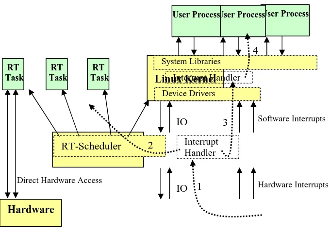
Figure 4: Interrupts in RTLinux
The handling of a hardware interrupt is shown in Figure 4. Each dotted arrow depicts one of the following steps.
1. A hardware interrupt is generated. The interrupt handler in the RTKernel receives the interrupt. 2. The interrupt handler in the RTKernel will check if an ISR is installed for that interrupt. If an ISR
is available it will be executed.
3. When no ISR is available in the RTKernel a software version of the original hardware interrupt will be generated in the Linux kernel.
4. The interrupt handler in the Linux kernel will check if an ISR is installed. If the ISR is installed it will be executed. When no ISR is available the interrupt will be ignored.
2.2 Communicating Threads for C++
Communicating Sequential Processes (CSP) is founded on mathematical theory, which gives it a good basis for developing reliable concurrent and distributed software. CSP allows the description of systems by means of processes that communicate with each other over channels (Hoare, 1985). CSP hides the thread programming from the user because programming threads is hard to do and errors are easily made. Threads are low-level entities, which makes understanding and controlling the flow of control of concurrent tasks difficult and as a result, the complexity and development times may increase extensively, reducing development time and development costs (Hilderink, 2001).
In the Communicating Threads for C++ (CTC++ or CTCPP) library, an API that implements a subset of CSP is defined (Hilderink, 2001). The library makes CSP applicable for building concurrent software in C++ without a need to understand the underlying theory. CTC++ provides all ingredients for programming concurrent software. One can efficiently control threads without programming the threads directly. CTC++ puts the thread control to a higher level of abstraction in terms of
communicating processes. Its simple compositional constructs and features make reasoning, designing and building concurrent programs simple and especially reliable. The complex thread control lies
RTLinux Kernel RT-Scheduler
Hardware Interrupts IO
Software Interrupts IO
Linux Kernel
Device Drivers System Libraries
Direct Hardware Access
Hardware
User Process User Process
User Process
RT Task RT
Task RT
Task
1 2
3 4
under the hood of these constructs. As a result, the development time scales nearly linear with complexity (Hilderink, 2001).
There are several terms used in CTC++, of which the essential ones are given below.
Processes
A process is an independent self-contained entity that performs a task (sequence of events) within its private workspace to achieve a certain goal and during its progress it may interact with its
environment by means of channel communications (Hilderink et al., 1999). Processes can be composed of multiple simpler processes. Processes do not know each other’s name and cannot directly alter each other’s state.
Channels
A channel is a shared object that performs communication between processes. Channels provide synchronization, scheduling and the actual data transfer. Each channel supports one-way point-to-point synchronous communication between processes. The communication is synchronous, so for one process to be able to send over a channel, the process at the other end must be ready and waiting for the communication. The channel connects the two processes. During channel communication one context switch is performed. The notion of a channel abstracts away from the actual physical
implementation of the communication link. Communication over a channel is by default rendezvous, but linkdrivers can be used to add buffering and hardware communication to a channel. Buffering is an option that may in certain circumstances increase performance.
2.2.1 Producer – Consumer Example
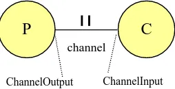
In the example shown in Figure 5, two processes are shown: the producer and the consumer. The two processes are running in parallel. The producer transmits data over the channel to the consumer. This can only be done if both the producer and the consumer are ready to communicate. When one of the processes is not ready to perform the communication, the ready process, will block and wait until the other process is ready. So the two processes will be scheduled and released on channel
communication. When the second process becomes ready for communication, both processes will continue their execution.
channel
ChannelOutput ChannelInput
C
P
Figure 5: Producer – Consumer example
Linkdrivers
The CTC++ package provides a linkdriver framework. The purpose of the linkdriver framework is to perform the separation between hardware-dependent and hardware-independent code in such a way that it fits neatly into the concept of channel communication. The idea is to accomplish this by creating a plug and play driver framework that continues on the conceptual idea of communication at a lower level. Just as a process reads from or writes to a channel, a channel reads from or writes to a linkdriver. The result of this is that the hardware dependency is completely hidden inside the
Figure 6: Linkdriver concept
Compositions
There are a few fundamental processes that can specify the relation between certain processes. These are the Sequential, Parallel, Alternative, priority-based Parallel (Priparallel) and priority-based Alternative (Prialternative) constructs. Since the compositions are processes themselves, they can be nested. In case of Priparallel constructs, this could result in an infinite amount of priority levels. A description of the compositions is discussed next.
• The Sequential construct executes its processes in sequence. The sequence starts when the run method is called. When all the processes of the sequential construct have terminated successfully, the sequential construct will terminate itself. A code example is shown below.
void main(void)
{
...
...// create processes and channels ...
Process *processlist[] = { process1, process2 }; Sequential *seq = new Sequential(processlist, 2); seq->Run();
... }
• There are two parallel constructs. The standard Parallel and the Priparallel. The Parallel
composition is started when its run method is called. This will run all the specified processes in parallel. Each process is assigned a thread of control with equal priority. Only when the Priparallel composition is used, the assigned threads will have different priorities. The first process in the list of the Priparallel will get the highest priority. When all processes have terminated successfully, the parallel composition will end. A code example is shown below.
void main(void)
{
...
...// create processes and channels ...
Process *processlist[] = { process1, process2 }; Parallel *par = new Parallel(processlist, 2); par->Run();
... }
Software Process
Hardware Process Channel
linkdriver Hardware dependent
• The alternative construct also has two versions: a standard Alternative and a Prialternative. The alternative composition is included to support non-determinacy for channel usage. This
composition gives a process a choice to read from one of a number of channels. Which channel is to be determined by the guards. Guards are objects which each guard a process. When a channel becomes ready for communication, because a process has written to it, it will signal the guard. The guard now becomes ready. When the alternative composition is executed, it will check the guards and choose between one “ready” guard and execute the corresponding process. The sequence in which the guards are handled is not determined, but in CT it is first come first serve. When the Prialternative construct is used the first process in the list will have priority over the other processes. The first code example shown below is a manager process. This process creates two guards for the reader processes. As soon as one of the guards is ready, the reader belonging to that guard will be executed.
void Manager::Run(void) {
...
guard1 = new Guard(in1, reader1); guard2 = new Guard(in2, reader2);
Guard[] *guardlist = { guard1, guard2 }; alt = new Alternative(guardlist, 2); ...
}
In the next code example the manager process is running in parallel with two producers. It is not known which producer is the first to become ready. When a producer is ready, it will signal the guard of its reader process. This reader process will then be executed.
void main(void) {
...
...// create processes and channels ...
Process *processlist[] = { producer1, producer2, manager }; Parallel *par = new Parallel(processlist, 3);
par->Run(); ...
}
Scheduling
A process that wants to access a channel that is not (yet) ready will be descheduled until the channel becomes ready. Waiting on a channel does not consume time (except for the context switch) because other processes can continue. So all processes that are dependent on communication from other processes will be descheduled until their channels become ready. A parent process schedules a child process when the run method of the child process is executed. If a process reaches the end of its run method, it will automatically be descheduled.
2.3 20-Sim
The code generation is done for a specific target. Every target has it own requirements and ways to be initialised and handled. So for every target a specific template has to be written. To be able to generate RTLinux C++ code one of the existing templates of 20-sim had to be adapted. Gerald Hilderink did this.
20-sim can generate code for the entire model or for sub-models in sequential execution frameworks. The code is based on a simulator framework, which is purely sequential and therefore inherits all the disadvantages of a single thread of control. The 20-sim code generation has been adapted in such a way that every sub-model can be code-generated individually and each sub-model is wrapped by a CSP process. Each process executes its own sub-model and the entire framework of the program can be composed using processes and CSP primitives. This allows executing sub-models (processes) in sequence, in parallel, or by choice. These sub-models can also be executed at different priorities in order to meet certain real-time constraints.
20-sim is used to simulate the entire system from setpoints to plant. With the simulation a controller with desired behaviour can be designed. When the design phase is completed the 20-sim is used to generate the code needed to implement the controller.
2.4 Setup IO Interface
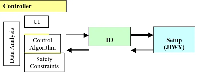
As shown in Figure 7 the complete setup consists of a Controller, IO and a plant (JIWY).
Figure 7: General Control System
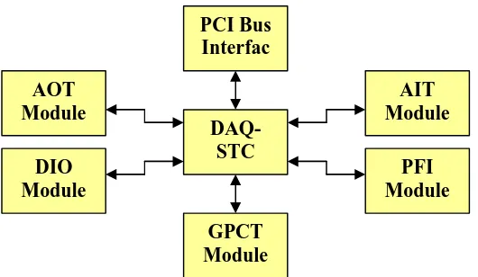
Every controlled plant has sensors and actuators, connected to the controller. In order to do this an IO board was needed. From several alternatives the NI6024E was chosen as the interface board to connect the controller to the sensors and actuators. The list with all the interface boards, from which this IO board was chosen, can be found in Appendix C. The NI6024E is a fast data acquisition (DAQ) board from National Instruments. The following modules, shown in Figure 8 are available on the board:
• The PCI bus interface.
• The Data Acquisition System Timing Controller (DAQSTC). • The Analog Input Module (AITM).
• The General Purpose Counter / Timer (GPCT). • The Digital IO module (DIO)
• The Analog Output Module (AOTM). • The Programmable Function Inputs (PFI).
The abbreviations are used in the manuals of the IO board and for the conformity they are used in this document as well.
Controller
Safety Constraints
Control Algorithm
Data Analysis
IO Setup
Figure 8: Component Connection Diagram
The interface board has a total maximum sample rate of 200K samples/s. 8 differential or 16 single ended analog inputs with 12-bit resolution and 2 analog outputs with 12-bit resolution are available. 2 timer / counter modules and 8 digital IO lines are also available. Programmable function inputs are available, although the other modules may use certain pins of the PFI for their own functions.
The DAQSTC is a timing module that can be programmed to generate all the necessary timing signals to drive the other modules on the board. The AITM can be used to measure voltages from sensors, while the AOTM can be used to drive amplifiers needed for motors. The GPCT can be used for timing (e.g. frequency measurement) and counting of various signals (e.g. event counting). They can also be used to interface digital relative optical position encoders. The DIO lines can be used to measure or drive digital signals. The PFI module can be programmed in such a way that external signals can be used as internal trigger signals for the other modules on the IO board. The details of the functions will be discussed in section 3.1.
2.5 Review
In this chapter the development environment was introduced. The development environment is the combination of hardware and software tools, which were used to develop the control software.
The first part of the environment that was introduced is RTLinux. This is a hard real-time version of the standard Linux operating system. RTLinux can facilitate the timing requirements needed for real-time processes and also provides all the facilities of the Linux OS. A communication mechanism between the two kernels was introduced. This mechanism uses RT-FIFOs for the communication.
The second part of the development environment is the CTC++ package. This package is an implementation of CSP concepts in C++. With CTC++ fast and reliable real-time software can be developed in a short time. The most important terms of CTC++ were introduced and explained.
The simulation and modelling package 20-sim is the third part of the development environment. With 20-sim models of physical systems can be modelled and simulated. Controllers for the models can be designed and then tested with the model. The latest versions of 20-sim have code generating abilities, so the designed models or controllers can be implemented in code, which is generated automatically.
The fourth and last part of the environment is the IO board. A selection from several IO boards was made and a data acquisition board from National Instruments was selected. On the IO board two analog outputs, 16 analog inputs, two counter/timers and a digital IO port are available. All the modules are connected to the central timing chip that controls the timing for the entire IO board.
PCI Bus Interfac
e AOT
Module
AIT Module
DAQ-STC
PFI Module DIO
Module
3 Software Development
With the help of the development environment, described in chapter 2, software has been developed.
The most important part of the developed software is the device driver for the IO board. Without it no connection between the controller on the PC and the actual setup can be made.
In order to make the system easier to use support utilities have been created. These utilities can be used to test the four most important modules of the IO board, to enable the RT-FIFO communication, to print messages to the screen and to log data to the hard disk.
Two programs to test RTLinux and the CTC++ package are developed as well. The programs measure the channel communication time and the interrupt latency. The results are given at the end of the chapter.
3.1 Data Acquisition Board Device Drivers
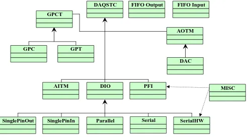
The used data acquisition board (DAQ) contains several modules, which are all interconnected through the DAQSTC module. For each of the modules classes have been created which control each part of the hardware so that the functions can be performed from software. The details of all the classes can be found in the documentation generated with CPPDOC. The relation between the classes is shown in Figure 9.
Figure 9: Class Relation Diagram
The DAQSTC class is the most important class. All other classes, except for the FIFO classes, are dependent on the DAQSTC class. From the DAQSTC there are six sub classes:
• GPCT.
The GPCT has two sub classes, namely the GPT and the GPC. These classes implement the timer and counter units.
• AOTM.
The AOTM has one sub class: the DAC class. The DAC class implements the DAC units. • AITM.
DAQSTC FIFO Output FIFO Input
GPCT
GPT GPC
AOTM
DAC
DIO PFI
AITM
SinglePinOut SinglePinIn Parallel Serial SerialHW
The AITM class is the implementation of the analog input. • DIO.
The DIO class has five sub classes. The two SinglePin classes implement the single pin IO mode. The parallel and serial classes implement the parallel and serial IO modes respectively. The SerialHW class implements the serial IO mode with a hardware clock.
• PFI.
The PFI class implements the PFI functions. • MISC.
The MISC class implements some functions that are needed by the SerialHW and PFI classes. Next there are the two FIFO classes. These classes implement the RT-FIFO communication between the RTLinux and the Linux processes.
3.1.1 System Timing and Control Module
The System Timing and Control module (DAQSTC) controls all of the modules and gives the user access to the registers on the board. Through the registers the modules can be programmed to perform the available functions. The details about bit settings for the various functions can be found in the manuals of the IO board (NI6024E, 1995, 1998). The DAQSTC object has only one implemented method: Initialise. This method will initialise the shadow registers for the register access and perform the PCI bus initialisation. The class and methods are shown in Figure 10.
Figure 10: DAQSTC class
Register Access
Some registers can be read directly, because these registers must be fast since they are frequently used. The other registers are accessed in a windowing scheme. Windowing requires two IO operations for each register, in favour of fewer addresses. This was done to preserve compatibility with older boards and to limit the size of the IO address space (i.e., IO window). These windowed registers are primarily used for setup functions, while the direct addressable registers are used for data acquisition. The addresses of all the registers and their functions can be found in the DAQSTC reference manual and the Register Level Programmers Manual (NI6024E, 1995, 1998). These register addresses are defined in the file NI6024E.h.
In order to minimize the number of used register addresses on the IO board, in addition to windowing registers were given a double function. When a read to an address is invoked, the appropriate read-only function register is selected. When a write to the same address is started, the write-read-only function register is accessed. This greatly reduces the number of addresses. This implies that a write-only register can’t be read to see what settings are made. So a way of storing all settings for read back was created. Every time data is written to a write-only register, the data is also written to a software copy of that register, which is kept in memory. Each register read or write has a register name, a value and a READ/WRITE flag. When a read occurs on a write-only register and the WRITE flag is included, the content of the software copy register is returned. The same applies in reversed form for the write on a read-only register. This software copy scheme is build into the read and write methods. Some of the registers are strobe registers. This means that when a bit in the register is set once and immediately cleared afterwards. To correctly use these registers, the software copy must not be updated. A strobe method was written to deal with this. The prototypes of these functions are described in Appendix E. The functions are located in the NI6024E.h file.
PCI Initialisation
The DAQSTC also handles the communication with the PCI bus. PCI read/write routines can be used to communicate with a PCI board, since the PCI bus interface handles all the communication between
DAQSTC
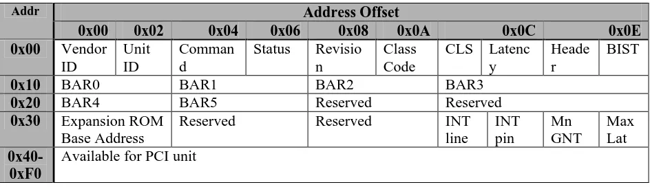
the PCI bus and the PC. Rubini (Rubini, 1998) shows how the BIOS in the PC maps the IO space of the PCI board to certain regions in the IO space of the PC during boot time. The start addresses of these regions are located in the Base Address Registers (BARs). These BARs are located on the PCI board. By means of BIOS-PCI functions, the contents of the BARs can be read. The PCI
configuration memory is structured for every PCI board as shown in Table 1. The addresses shown are 16 bit addresses.
Address Offset Addr
0x00 0x02 0x04 0x06 0x08 0x0A 0x0C 0x0E
0x00 Vendor ID
Unit ID
Comman d
Status Revisio n
Class Code
CLS Latenc y
Heade r
BIST
0x10 BAR0 BAR1 BAR2 BAR3
0x20 BAR4 BAR5 Reserved Reserved
0x30 Expansion ROM Base Address
Reserved Reserved INT line INT pin Mn GNT Max Lat 0x40-0xF0
Available for PCI unit
Table 1: PCI Configuration Memory
The BIOS maps the IO space of the PCI board to the upper limit of the IO space of the PC. To be able to access the PCI board with the conventional read/write functions of C and C++, its IO space must be remapped to a new memory segment. The Initialise method searches the PC for a PCI bus and, if present, for the IO board. When the IO board has been found, the two BAR addresses (BAR0 and BAR1) used by the NI6024E will be read from the board and remapped to the following base addresses: Base Address0 = 0xd0000 and Base Address1 = 0xd1000.
3.1.2 Analog Output Timing Module
The analog output timing module (AOTM) has two bipolar analog output channels. The Digital to Analog Converters (DAC) in these channels can generate an analog voltage from –10V to +10V with a resolution of 12 bits. The AOTM has two main modes: DAQSTC driven mode and CPU driven mode. In DAQSTC driven mode the AOTM can be fully programmed to generate any waveform desired. However, this requires the entire waveform to be known in advance, which is not applicable in control applications. In the CPU driven mode the CPU can directly write to the DACs on board of the NI6024E. The CPU driven mode has been fully implemented. The AOTM object has several methods used for the setup of the module. When the AOTM has been initialised in the CPU driven mode the DAC object can be requested from the AOTM with the GetDAC method. Two DAC objects can be requested from the AOTM: DAC0 and DAC1. The write method implemented for the DAC objects generates the corresponding voltage on the output when called. The write method can be called with a value that must be between –2048 and 2047. Values that are out of this range will be corrected to the maximum values. The classes and their methods are shown in Figure 11.
Figure 11: AOTM and DAC class
3.1.3 Analog Input Timing Module
The analog input timing module (AITM) has 16 uni-polar input channels. These channels can also be used in bipolar mode, which requires two uni-polar channels. The resolution of the Analog to Digital Converters (ADC) is 12 bits. Just like the AOTM, the AITM can be fully programmed for a scan sequence. The used gain is software selectable. Note that the input range of the channel is dependent on the gain. The details can be found in the manuals (NI6024E, 1998). The AITM is not working. After several weeks of programming it still did not work and other people could not find any faults. Since it is not used for this project at the moment it is left as is. Only the AITM object has been implemented. This object has no implemented methods. The class and methods are shown in Figure 12.
Figure 12: AITM class
3.1.4 Digital IO Module
The Digital IO module (DIO) consists of one 8 bits port. This port can be used as input or output, in various modes. The supported modes are:
• Parallel IO without a hardware clock. • Serial IO without a hardware clock. • Serial IO with a hardware clock.
The parallel IO mode can also be used to drive each pin individually, so a “virtual” single pin mode can be used. Note that Pin 6 and 7 can also be used as up/down inputs for the counters. If this is the case the parallel IO mode cannot be used! The SerialHW mode needs a clock to operate. This clock function is located in the MISC class. See the documentation for the class details. The DIO object must be created while specifying which mode to use. An object depending on the specified mode is created. For each of the modes read and write methods are created. These methods are linked to the read and write methods of the DIO object. This holds for the Serial and Parallel modes, but not for the SinglePin modes. Since 8 pins are available 8 SinglePin objects can be created. Linking the read and write methods to the DIO object will not work There is only one DIO object with one read or write method and there can be eight singlePin objects, so read and write methods are implemented in the SinglePin objects themselves.
The Serial, Parallel and single pin modes are fully implemented. The Serial hardware clocked mode depends on the clock setup, which is not implemented since it was not used The DIO class and its sub-classes with all the methods are shown in Figure 13.
3.1.5 Counter / Timer Module
The General Purpose Counter/Timer module (GPCT) contains two units, each of which can be used as counter or timer. The resolution of the two units is 24 bits. The counters can be used for counting signals, which are routed from the input, or from signals of the other modules on the NI6024E. In combination with the pins 6 and 7 of the DIO module an up/down counter can be created for digital incremental encoders. The timers can generate timing signals that can be routed to the outputs or to other modules of the NI6024E. The GPCT object has only two methods: GetTimer and GetCounter.
When the Counter object is created it can be configured for the RelativePositionSensing mode. In this mode the counter in combination with pins 6 and 7 of the DIO module form two up/down counters. When this mode has been initialised (the position is initialised to “0”.) the counters must be armed to start counting. Disarming the counters will make them stop counting. The last value remains in the counter register until a reset is performed or the counter is armed again.
Only the counters of the GPCT are implemented, since the position encoders generate pulses with a direction signal. For the counters only the relative position sensing method has been implemented. The GPCT class and the sub-classes are shown with their methods in Figure 14.
Figure 14: GPCT, GPC and GPT classes
3.1.6 Programmable Function Inputs Module
The Programmable Function Inputs (PFI) pins can be used as inputs for external generated timing signals. These pins can internally be routed to any of the timing signals needed for any of the modules. These pins can also be used as outputs, where they supply the internal timing signals to the outside. The PFI object enables the modules to use an external signal as source for a timing signal. The constructor needs a pin number and an IO direction. The specified pin will then be put in the right mode. In the setup of the other modules, these modules can be configured to use a PFI pin as source or destination for a timing signal. The PFI pins are fully implemented. The class and methods are shown in Figure 15.
Figure 15: PFI class
3.1.7 Miscellaneous Functions
The miscellaneous functions are embedded in the MISC class. This class has three methods:
• MSC Clock Configure. This method configures the clock for the serial IO with hardware clock. • MSC FOUT Configure. This method configures the FOUT register settings for the analog input. • Analog Trigger Control. This method configures the settings for the analog trigger control. The class and methods are shown in Figure 16. These three methods are used for other modules, however not for one other module but several modules. In the manuals these functions are stated as
GPT
GPT() ~GPT()
GPC
GPC(Counter,Mode) ~GPC()
Arm() Disarm() SetMode(Mode) GetCounterValue() GetSaveRegister() Initialize(Counter,Mode) Read()
Reset() Counter Mode GPCT
GPCT() ~GPCT()
GetCounter(Counter) GetTimer(Timer) Counter Timer
PFI
PFI(Pin, IOdirection) ~PFI()
miscellaneous functions. The functions could have been implemented in each of the classes that use them, but for conformity a MISC class was created.
Figure 16: MISC class
3.2 Support Utilities
Apart from the device drivers for the IO board four support utilities were needed. The utilities are: • Test utilities for the analog input, analog output, digital IO and the encoders.
• RT-FIFO communication.
• A program to print messages to screen. • A data-logging program.
3.2.1 Test Utilities
The test utilities are designed to test the DAQSTC and the modules. With the utilities the correct operation of other connected hardware can be tested. There are four test utilities: ADC, DAC, DIO and ENCODER.
• ADC is the test program for testing the analog input system. This is not implemented because the AITM module is not working.
• DAC is the analog output test program. It will test both the DAC channels in their full range. When the program is started, the output of DAC0 will start at 0V and rise to the maximum, while DAC1 will start at 0V and fall to the minimum. Then the DAC0 will fall from maximum to the minimum. DAC1 will do the opposite. Next both the DACs will return to 0.Connecting the output to an oscilloscope can show the actual signals.
• DIO is the Digital IO test program. The program will output the value 0 to 255 on the eight digital IO lines. Eight LED’s connected to the port can be used as a display.
• ENCODER is the test program for the counters and clock converter electronics. When started it will read the value of the digital incremental encoders and print that value to the kernel buffer. This step will be repeated 50 times.
3.2.2 RT-FIFO
Since the Linux kernel can be pre-empted by a real-time task at any moment in time, no Linux routine can safely be called from real-time tasks. The RTLinux kernel provides simple buffers and they are used for passing information between RTLinux processes or between Linux processes and RTLinux processes. These communication buffers are called real-time FIFOs (RT-FIFO). RT-FIFO buffers are allocated in the kernel address space. The real-time task interface to RT-FIFOs includes creation (rtf_create), destruction (rtf_destroy), reading (rtf_get) and writing (rtf_put) functions. Reads and writes are atomic and do not block (Barabanov, 1996). Non-blocking avoids priority inversion. For the RT-FIFOs handlers can be created. The handlers function exactly like an interrupt handler, only these handlers react on read/write actions on RT-FIFOs instead of interrupts Two types of RT-FIFO handlers are available.
The function
int rtf_create_handler(unsigned int fifo, int (* handler)());
creates a handler, which is called when data is read from or written to RT-FIFO fifo from the non real-time side. The second function
int rtf_create_rt_handler(unsigned int fifo, int (* handler)());
creates a handler, which is called when rtf_put or rtf_get is called on RT-FIFO fifo. Linux MISC
MISC() ~MISC()
processes see RT-FIFOs as ordinary character devices. The full features of the Linux API can be used to access the devices.
The RT-FIFOs are implemented in two FIFO classes: FIFO_Output and FIFO_Input. The FIFO classes specify a read and write method, which can be used to communicate via the RT-FIFOs. The FIFO classes transmit objects. Data to be transmitted must be cast to an object. On the other side of the RT-FIFO the object must be cast to the original type. The two function calls show how this is done.
fifo-object1->write((void*)&data, sizeof(data)); void* data=fifo-object2->read();
Details about the classes can be found in the documentation. The two FIFO classes are shown in Figure 17.
Figure 17: FIFO Input and Output classes
3.2.3 Console
In a real-time module, the standard print statements cannot be used since this function is designed to operate in user space and not in kernel space. Instead the real-time version (rtl_printf) of the
statements can be used. The only drawback is that these print statements are directed to the kernel buffer. The contents of the kernel buffer can be printed to the screen with the “dmesg” command. Console provides a means of printing messages from the real-time program via RT-FIFOs to the screen. This is graphically depicted in Figure 18.
Figure 18: Console communication method
On the real-time side, there are four functions available in the console package, which is located in the file rtl_console.c. The functions are discussed below.
• int fd = rtl_console_open(int rt-fifo);
This function opens the RTFIFO rt-fifo, and returns the pointer fd to the opened RT-FIFO. This function must be called in the “init_module” section.
• rtl_console_printf(int fd, const char* format, …);
This function behaves exactly like the printf and rtl_printf statements. The same formatted arguments can be used. The only difference is that the pointer fd has to be specified.
• rtl_console_kill(int fd);
This function sends a termination command to the non real-time side. This will close the non real-time side client. This function must be called in the main program and not in the
“cleanup_module”. When the “cleanup_module” is called, all resources are freed. When the non real-time client has the RT-FIFO opened, the resources cannot be freed and the
“cleanup_module” will fail.
• rtl_console_close(int fd);
This command will destroy the RT-FIFO. This function must be called in the “cleanup_module” section of the real-time program.
RT Process
Console (Linux Process)
RT-FIFO
FIFO_Output
FIFO_Output(RTFIFO) ~FIFO_Output() Write() RTFIFO
FIFO_Input
When the real-time process is started, the non real-time program, called “console” can be started. If the program is started without any switches the program will try to connect to RT-FIFO 63 by default to read the data. By specifying a switch, another RT-FIFO can be selected. E.g. "./console 2". Console will print all the messages from the RT-FIFO to the screen. The program can be stopped by pressing Ctrl-C on the non real-time side or by sending the “kill” command from the real-time side.
3.2.4 Logger
Logger is a program that reads data from the RT-FIFOs and writes that data to a file. The data is stored in a format that 20-sim can read. This way, measurement data can be displayed in 20-sim. In the logger directory there are two “.c” files: logger.c and logger2.c. Both the files read a different format from the RT-FIFOs. To use the program a priori knowledge of the type of the transmitted variables is needed. The loggers expect data from each of the RT-FIFOs in the formats shown in Table 2 and Table 3. Note that the number of samples (n) and the number of RT-FIFOs (f) are not fixed. There can be a total of 64 RT-FIFOs.
Logger.c transmits two values per RT-FIFO per iteration: namely one integer and one long double. Number of RT-FIFOs Þ (f)
RT-FIFO x RT-FIFO x+1
index (integer) data (long double) index (integer) data (long double)
1 … 1 …
2 … 2 …
3 … 3 …
Samples
Þ
(n)
4 … 4 …
Table 2: Logger data format
Logger2.c transmits the index (an integer) through the first RT-FIFO while the other RT-FIFOs are used to transmit the data (long doubles).
Number of RT-FIFOs Þ (f)
RT-FIFO #1 RT-FIFO #2 RT-FIFO #3 RT-FIFO #4 index (integer) data (long double) data (long double) data (long double)
1 … … …
2 … … …
3 … … …
Samples
Þ
(n)
4 … … …
Table 3: Logger 2 data format
The real-time program must be started before the logger program, otherwise the logger program will generate an error since the RT-FIFOs are then not yet created by the real-time program. The logger program will loop forever, until Ctrl-C is pressed.
At the real-time process the data must be transmitted through the RT-FIFOs. This is done in exactly the same way as shown in section 3.2.2. On the non real-time side the logger program must be started with the following command:
./logger [switches]
The switches are required and must be the two following types. The order is not important.
-f fifos where fifos are the numbers of the RT-FIFOs to use in the specified order. There are 64 RT-FIFOs with numbers from 0 to 63.
An example of the command is:
./logger –o testdata –f 0 1 23
This will save the data read from RT-FIFOs 0, 1 and 23 to the file testdata.n. The “data file” options in 20-sim can easily read the contents of the file.. However, take note that when other programs are used to read the file, a problem with the decimal separator may occur since Linux uses “.” and other operating systems may use “,”. This will result in strange numbers. When 20-sim is used, this will cause no problem.
Minimum RT-FIFO Size
The logger runs on the Linux kernel, therefore it must be considered that the non real-time logger will not get any CPU time, because the RTKernel consumes all of it. When this happens, the RT-FIFO must have enough space to store all the data, otherwise errors are generated in the real-time process. All variables require a certain amount of space in memory to be stored. The amount of space needed for every type of variable differs, also the same type of variable can use more or less space on different operating systems. In Table 4 the sizes of the various variable types for the Linux operating system are shown.
Variable Type Size in Bytes (Linux)
CHAR 1
SHORT 2
Unsigned SHORT 2
INT 4
Unsigned INT 4
Long INT 4
LONG 4
Unsigned LONG 4
FLOAT 4
DOUBLE 8
Long DOUBLE 12
Table 4: Variables storage size
As can be seen the long double is the largest variable. With the known sizes equations on the RT-FIFO size can be created. If we have a sample frequency of “f’ Hertz and the controller will run “t” seconds, this will result in “n” sample moments where ‘n” is:
f t
n= ∗
Equation 1: Number of sample moments
If all the data and one index is transmitted through only one RT-FIFO the buffer size of the RT-FIFO will be:
(
v
ldouble
)
n
bytes
Buffsize
(
)
=
∗
1
∗
int
+
∗
Equation 2: Buffer size
where n is the number of sample moments, int is the size of an integer, v is the number of variables to log and ldouble is the size of a long double.
Logger 1 uses one RT-FIFO per variable, but it transmits an index and a data value per RT-FIFO. For logger 1 the sizes of the RT-FIFOs can be calculated with the following equation:
(
ldouble
)
n
ze
FIFObuffsi
DataRT
−
=
int
+
∗
Equation 3: Data RT-FIFO size for logger 1
As discussed logger 2 uses one RT-FIFO for an index and a RT-FIFO for every variable. For logger 2 the sizes of the RT-FIFOs can be calculated with the following equations:
n ze
FIFObuffsi
IndexRT− =int*
Equation 4: Index RT-FIFO size for logger 2
n ldouble ze
FIFObuffsi
DataRT − = *
Equation 5: Data RT-FIFO size for logger 2
As can been seen from Table 4 the storage size of an integer int is 4 bytes and the size of a long double ldouble is 12 bytes.
An example: 2 variables are logged. The sample frequency f is 100Hz. The program run time t is 10s. According to Equation 1 the number of sample moments n is 1000.
The resulting RT-FIFO sizes are shown in Table 5.
RT-FIFO 1 size (bytes)
RT-FIFO 2 size (bytes)
RT-FIFO 3 size (bytes)
Logger 1 1600 1600 (Not used)
Logger 2 4000 1200 1200
Table 5: Buffer sizes
The size of the RT-FIFOs is reduced at the cost of more RT-FIFOs to be used. If all the data is transmitted through one RT-FIFO its size will be 3200 bytes for logger 1 and 2800 bytes for logger 2.
3.3 System Test Programs
In order to do some tests on the system, without any test case dependent code, two test programs were created. The first program is a real-time version of the Comstime program. The second program is designed to measure the interrupt latency under the real-time kernel.
3.3.1 Comstime
The CTC++ package contains an example benchmark program called Comstime. Comstime is designed to calculate the time needed to perform channel communication. For the benchmark on the RTLinux system, a real-time version has been created. The program consists of four processes, connected as shown in Figure 19. The program works as described below.
Figure 19: Comstime Program Structure 0
T i++
The ‘0’ block outputs a 0 on the first run, but on subsequent runs this block will output the value received on the input. The ‘delta’ block copies the value of the input to both of the outputs. The ‘T’ block records the time, when it receives the input from the ‘delta’ block. The ‘i++’ block will increment the input value by one and transmit it to the ‘0’ block. Each arrow signifies a channel on which the data is transported. Communication over one channel requires one context switch. The PAR statement inside the ‘delta’ block also requires one context switch. In total there are five context switches per loop. The program will perform the loop until the ‘T’ block reaches 1000. The total program execution time thus stands for 5000 context switches with channel communication.
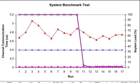
The Comstime benchmark was performed under different conditions. It was performed under
RTLinux firstly with a system load of 100% and secondly with a load of approximately 1-2%. Letting the “grep” utility recursively search in all the files on the hard disk, for the string “a”, generated the system load. Three of these processes were started. The load on 1-2% is the normal load when no user processes are running. The benchmark was also performed on the same machine running under DOS. The DOS system utilized a system load of approximately 1%. The results of the benchmarks are shown in Figure 20.
Figure 20: Comstime Benchmark Results
As can been seen from Figure 20 the picture, the channel communication time (with context switch time!) for DOS remains constant. The channel communication time for RTLinux varies somewhat when the system load is 100 percent. When the load is dropped to 1-2%, the variation of the channel communication time is decreased. In a real-time context the worst case is the most important. The worst-case channel communication time is 5,06 microseconds. Unfortunately the system load under DOS cannot be increased since DOS is a single task OS.
System Benchmark Test
4 4.2 4.4 4.6 4.8 5 5.2
1 2 3 4 5 6 7 8 9 10 11 12 13 14 15 16 17
Run
Channel Communication
Time (us)
0 10 20 30 40 50 60 70 80 90 100
Ssytem Load (%)
3.3.2 Interrupt Latency
An example program from a Real-time Linux website (Holler, 2000) shows the interrupt latency by means of a simple program. The program requires a few wires connected to the parallel port and an oscilloscope as shown in Figure 21.
Figure 21: Test Hardware schematic
Pins 2 and 3 are the two least significant bits of the 8 data bits. Pin 10 is the acknowledge input of the port and pin 25 is the ground of the port. With the above connection, the software can generate a hardware interrupt on the parallel port by means of setting pin 3 in a high state. The instruction to put pin 3 in a high state also puts pin 2 in a high state. Since pin 2 is connected to the oscilloscope, the level of the pins can be seen.
An interrupt handler responds to the caused interrupt by putting pins 2 and 3 in a low state, and thus disabling the interrupt. The transitions can be seen on the oscilloscope. The program was started as a periodic thread, which was scheduled to run every 100 µs. This results in a steady picture on the oscilloscope, which looks like Figure 22. The times of the four points shown are stated in Table 6.
Figure 22: RTLinux Interrupt latency
System Load Idle Cycles (%)
t1 (ms)
t2 (ms)
t3 (ms)
t4 (ms)
High ? 1=t2-t1
Sample time ? 2=t3-t1
Low ? 3=t3-t2 No extras, just
X(-windows)
97 101 108 201 208 7 100 93
Camera, Mouse Interrupts & X
58.6 101 109 201 209 8 100 92
Load Function, Mouse Interrupts & X
0 101 109 201 209 8 100 92
Table 6: Interrupt Latency results
The system load that has been generated consists of IO operations that cause extra interrupts. Searching in all the files on the entire hard disk for the string “a” generated the system load: a continuous stream of interrupts. With 5 of these searches the total system load would reach 100%. The total cycle time (? 2) of the program is 100 µs. The fastest interrupt latency (? 1) with a system load as low as possible is 7 µs. For 100% system load the cycle time remains constant, but the interrupt latency increases to 8 µs. The worst-case interrupt latency is 8 µs. The latency time is regardless of the total load. The RTLinux kernel can schedule the program exact on the specified 100 µs.
? 2 ? 3 ? 1
t1 t2 t3 t4
Oscilloscope
On the website (Holler, 2000), where this test was found, test results for two PCs with the same test are shown. These results are shown in the following table with the above results. The mentioned Pentium Pro is the PC used for the project.
PC Average Latency
(ms)
Maximum Latency (ms)
Pentium II / 300 MHz 5 <10 486 DX2 / 66 MHz 35 65 Pentium Pro / 200 MHz 7.66 8
Table 7: Latency Comparison
As can be se