Volume 2010, Article ID 930327,16pages doi:10.1155/2010/930327
Research Article
A Relative-Localization Algorithm Using Incomplete Pairwise
Distance Measurements for Underwater Applications
Kae Y. Foo and Philip R. Atkins
School of Electronic, Electrical and Computer Engineering, University of Birmingham, Edgbaston, B15 2TT, UK
Correspondence should be addressed to Kae Y. Foo,[email protected]
Received 1 July 2009; Revised 5 December 2009; Accepted 13 January 2010
Academic Editor: Martin Ulmke
Copyright © 2010 K. Y. Foo and P. R. Atkins. This is an open access article distributed under the Creative Commons Attribution License, which permits unrestricted use, distribution, and reproduction in any medium, provided the original work is properly cited.
The task of localizing underwater assets involves the relative localization of each unit using only pairwise distance measurements, usually obtained from time-of-arrival or time-delay-of-arrival measurements. In the fluctuating underwater environment, a complete set of pair-wise distance measurements can often be difficult to acquire, thus hindering a straightforward closed-form solution in deriving the assets’ relative coordinates. An iterative multidimensional scaling approach is presented based upon a weighted-majorization algorithm that tolerates missing or inaccurate distance measurements. Substantial modifications are proposed to optimize the algorithm, while the effects of refractive propagation paths are considered. A parametric study of the algorithm based upon simulation results is shown. An acoustic field-trial was then carried out, presenting field measurements to highlight the practical implementation of this algorithm.
1. Introduction
The capability of reliable underwater modem technology
[1,2] has led to a growing number of emerging underwater
applications, presenting with them new possibilities and challenges. One of these applications is the deployment of a cluster of underwater sensors [3], which offers benefits ranging from oil-platform monitoring [4] to ecosystem monitoring, surveillance, and early warning systems for tsunami. A typical application of a sensor deployment generally involves the collection of data and the delivery of these data [5, 6]. In the former, the knowledge of sensor positions may play an important role in aiding the interpretation of the recorded data or in improving the performance of signal processing algorithms such as in array processing [7]. In the latter, where the collected data are sent or relayed to a destination, the estimation of sensor position enables the implementation of more energy and latency efficient routing and channelaccess protocols
[8,9]. Therefore, in situations where the positional
infor-mation are not available to the sensors prior to deploy-ment, or that it changes after deploydeploy-ment, there exists the
motivation to localize the sensors with existing modem capabilities.
(in tropical waters) to breaking waves in a stormy weather [14], thus contributing to a high and fluctuating level of ambient noise. These factors can potentially lead to incon-sistency in RSSI measurements. Similarly, measuring angles-of-arrival to a high accuracy may prove prohibitive unless every node is equipped with the necessary hydrophone array. The viable methods are therefore by using time-of-arrival measurements which require strict synchronization amongst all the nodes or by two-way ranging. The latter method requires no synchronization and operates by measuring the two-way propagation time assuming that the queried modem sends a reply packet after a fixed time-delay.
The task of underwater sensor localization can be considered as a two-step process; first by the localization of the sensors in the 3D Euclidean space with respect to one another using measurements of internode distances only, and then, if necessary, the anchoring of these positions to a reference or geodetic coordinate system. A relatively straightforward method of resolving the sensors’ relative locations using only pairwise distance measurements is by metric multidimensional scaling, as a special case where one assumes that the measure of dissimilarities is represented by Euclidean distances, and that a set of coordinates within the relevant dimensions explain the observed distances. This concept has its roots in the field of psychometrics [15], in which an early analytical solution was presented by Torgerson [16] and referred to as classical MDS. In order to apply classical MDS to the problem of sensor localization, all the pairwise distances between the nodes need to be obtained [17]. This implies that every node needs to have acoustic visibility to all the other nodes. Such a requirement may often be difficult to meet in practice, as ranging measurements may be erroneous or unsuccessful between nodes that are further apart, as well as nodes that are partially obstructed (such as by harbour walls) and have no complete visibility to all the other nodes.
The contribution of this article is in addressing the problem of relative localization using incomplete pairwise distance measurements. By applying a robust approach based upon an iterative, weighted, cost-minimization algorithm known as stress-majorization [18, 19], it is shown that a cluster of sensor nodes can be efficiently localized in the absence of complete pairwise distance measurements. The key improvements introduced herein are a robust and effective method of initialization of the algorithm, a parametric study of the proposed approach, and a case-study of its practical application based upon experimental field measurements. The next section relates the contribution of this paper with regard to previous research effort within sim-ilar domain.Section 3presents the analytical formulation of the problem and the algorithm of the proposed approach. In Section 4, simulation results provide a parametric evaluation on the algorithm’s performance. Section 5describes a field trial being conducted with 12 nodes using acoustic time-of-arrival measurements, capturing the issues related to the implementation of this algorithm and verifying the results predicted in the simulation study.Section 6presents a short discussion on the scope of this article whileSection 7draws the conclusion from this work.
2. Related Work
Sensor localization is an area of active research in both the radio [20–24] and underwater domains [25–29], where various solutions based on different levels of constraints and assumptions on infrastructure availability have been studied. Broader reviews on this subject can be found in [12,30].
In [23], Patwari et al. applied maximum likelihood esti-mation techniques to approximate a node’s relative location, but the accuracy of the approximations (and the validity of the derived lower Cramer-Rao bounds) depends on having complete pairwise distances for all the nodes and knowledge of the probability distribution underlying the observed data. Although one can assume that the pairwise distances are Gaussian distributed (the validity of which increases with higher signal-to-noise ratios [31]), the requirement of obtaining all pairwise distances may introduce a challenging constraint in practice for the application scenario considered in this article. In [22], Moses et al. also presented a self-localization approach method using a maximum-likelihood estimator, relying on both time-of-arrival measurements and angle-of-arrival measurements. It is also acknowledged that with incomplete data measurements, the maximum likelihood estimator may not yield a unique solution.
In [17], Shang et al. applied classical-MDS by eigenvalue decomposition (EVD) for the localization of nodes using distance measurements. It is demonstrated that closed-form solutions can be obtained without the need for iterative computations, but this is restricted by the condition that global information of pairwise distances in the network needs to be made available to a central processor or to all individual nodes. Ji and Zha [32] applied a majorization-MDS approach for sensor localization, allowing for missing pairwise distances. This removes the requirement for com-plete pairwise distance measurements. However, a random start configuration is applied for the estimation of the initial point coordinates, and the possible existence of non-linear propagation paths was not discussed. The work is extended by Costa et al. in [33], where arbitrary non-negative weightings can be applied to distance measurements, such that adaptive weightings can be applied to account for different levels of confidence amongst the pairwise dis-tances. The proposed algorithm is decentralised such that each node estimates its local cost function iteratively, then communicates this to their neighbours in order to achieve cost minimization globally across all the nodes. However, there is little emphasis on the method for estimating initial node positions, and the algorithm similarly assumes that the measured distances are an accurate representation of Euclidean distances between the nodes. Also, since the focus is on adaptively choosing neighbours based upon the quality of measurements by allocating the appropriate weightings, the work did not investigate the tolerance of the algorithm to varying levels of missing pairwise measurements.
of minimum distances were introduced. The key difference in their approach is in that a gradient descent algorithm was applied in the process of minimization, and that a multiple restart scheme was used to avoid local minima. Separately, an alternative method of addressing missing distances within a 3D environment was studied by Birchfield [35], which iteratively uses a subset of points (up to 4 for 3D) with the highest availability of distance measurements to derive an estimate of local coordinates, until all the coordinates based on relative distances are obtained. Simulation results showed that this can effectively mitigate the need for classical MDS in cases where the condition, that each node has a minimum of
m+ 1 unique distance measurements to nodes that satisfies the same condition, is met, where m is the total number of dimensions. This condition is more easily met when the total number of sensors is high compared to the number of dimensions which is usually only up to 3 in a Euclidean space. The focus of this work is on a majorization-MDS algorithm for the relative localization of underwater sensors, or nodes, by using only incomplete inter-node distance measurements, given no other a priori information. Central to this approach is the application of classical-MDS using approximated distances in replacement of missing pairwise distances for obtaining theinitialestimates of coordinates for the majorization algorithm. This is shown to be effective in avoiding local minima, and mitigates the need for multiple restarts with different sets of random estimates.
3. A Weighted and Iterative
Minimization Approach
Iterative majorization, a term coined by Heiser [11], is a minimization method formulated in the field of geomet-ric data representation [10, 18], and can be applied to multidimensional scaling [19, 36]. One of the attractive features of this algorithm is that a non-increasing sequence of function values are yielded, implying a quick and guaranteed convergence. However, it is worth noting that the algorithm does not necessarily converge at the global minimum. On the contrary, the point of convergence would, in most cases, be at a local minimum [37], hence the importance of having an effective approach to find the global minimum when applying this algorithm.
The sensor nodes are assumed to be stationary, or drifting at such a rate that the change in position during localization is negligibly small. Nodes are also assumed to have protocols to broadcast their presence to the other nodes, to perform mutual ranging measurements, and to share their range measurements with the other nodes. This assumption does not reduce the practicality of the algorithm proposed herein. In its simplest form, this can be based on a classical time-division protocol, where nodes broadcast their ID and any known pairwise measurements before performing ranging measurements to any previously unknown nodes, and repeating the process several times. Time-slots can be uniquely allocated based upon each node’s unique ID [38], while the slot length is defined in order to mitigate the need for strict time-synchronization across all the nodes. Optimized distributed protocols can be found in [33,39].
3.1. Problem Formulation. Relative-localization involves cal-culating a set of relative coordinates in the relevant dimen-sions of the Euclidean space for all the nodes within a cluster, such that their corresponding pairwise distances closely match the measured pairwise distances. Givennnumber of sensor nodes, the coordinates of these nodes are represented by ann×mmatrixXwheremis the number of dimensions. The pairwise distance between any two nodes is a function of the set of coordinatesX, and for a Euclidean space can be expressed as
di j(X)= ⎡ ⎣m
a=1
(xia−xja)2 ⎤ ⎦
1/2
, (1)
where di j is the pairwise distance between nodes i and j,
calculated using their respectivemdimensional coordinates. The elementsdi jform a symmetricaln×npairwise distance
matrix,D. Similarly, the measured distances between nodesi
and j,δi j, form a symmetrical pairwise distance matrix Δ.
The mismatch between the measured distances and those which are calculated for the approximated coordinatesXmaj can be expressed as
σ(X)=
i< j
wi j
δi j−di j(X) 2
, (2)
where wi j is the weighting for the distance between node
i and j that corresponds to element (i, j) in both the matrices Δ and D. The condition of i < j denotes the elements in the upper triangle of the symmetrical matrices. The weightings are normalized to values between 0 and 1 where a 0 represents a missing distance measurement. The functionσ is commonly referred to as the stress function in related literatures [40]. The remaining task is to approximate the coordinates of the nodes,Xmaj, such that the value ofσis minimized.
3.2. Classical-MDS. When all the pairwise distance measure-ments are available, classical-MDS offers a solution without iterative computations. Using the matrixΔ, the computation steps for classical-MDS [16,24] are given as follows.
(1) Calculate a covariance matrix, Z, from the square of the distance matrix, Δ2 by multiplication with centring matrices, producing a centred matrixZ = (−1/2)JΔ2JwhereJ=I−L/n,Iis an identity matrix of sizen, andLis a square matrix of ones of sizen. (2) Compute the eigenvalues,G, and eigenvectors,Q, by
applying eigen-decomposition onZ.
(3) The approximated coordinates, Xc, is then given by Qn,mGn,n1/2 where Qn,m is the firstn×melements
ofQ, whileGn,nis the firstn×nelements ofGthat
usually correspond to the non-negative eigenvalues in the diagonal.
3.3. Iterative Majorization Initiated by Approximated
Classical-MDS. If some of the pairwise range measurements
to the line-of-sight, then the measured pairwise distance matrixΔwill be incomplete (in which the elementsδi j that
correspond to the unavailable measurements are 0). In such cases, the function in (2) can be iteratively minimized by updated approximations ofXmaj. This is achieved by using a majorization function that satisfies a chain of inequality towards the stress function, resulting to new approximations ofXmajthat yield a smaller value for the stress function. The derivation of the majorization function is well documented in [36]. For the purpose of clarity in describing the proposed modifications, the usual procedures of the algorithm are herein described.
(1) Set the weightswi jcorresponding to thei-jpairwise
distances, using 0 for missing measurements and 1 otherwise, or, if a priori knowledge is available to provide indication towards the relative levels of confidence in the measurements, positive ratios of up to 1 are allocated.
(2) InitializeXmaj,0 to a set of random coordinates, and the number of iterations, k = 0, then calculate σ0 using (2).
(3) Calculate an update forXmaj,k by using the
relation-ship:
Xmaj,k+1=V+Bk
Xmaj,k
Xmaj,k, (3)
whereV+ =(V+L)−1
,Vis a matrix with elements
vi j formed from the allocated weightings such that
vi j = −wi j if i /=j and vii = nj=1,j /=iwi j for the
diagonal elements. Recall thatLis a square matrix of ones of sizen.Bkcontains elementsbi jcalculated in
the following manner:
bi j=
wi jδi j
di j
Xmaj,k
fori /=j, di j
Xmaj,k
/
=0,
bi j=0 fori /=j, di j
Xmaj,k
=0,
bii= n
j=1,j /=i
bi j for the diagonal elements.
(4)
(4) Calculateσk+1 and repeat from step 3 ifσk+1−σk >
h, where his an arbitrarily small positive constant acting as a threshold beyond which is indicative of a convergence, or ifk ≤K, whereK is the maximum number of iterations allowed. Otherwise, the relative locations are given by the coordinates in Xmaj,k+1. The corresponding distance matrix is Dmaj,RandInit. The value of hcan be set asσ0/105, such that it is suitably small to indicate that any further iterations yield negligible minimisation of the error parameter
σ, hence no further improvements to the estimate of relative positions.
3.4. Algorithm Optimization. A common method to
opti-mise the iterative algorithm inSection 3.3is to apply multiple restarts (i.e., performing the complete iterative algorithm repetitively) using different sets of random initial coordinates in order to avoid local minima. This may be computationally intensive for embedded processors on deployable nodes, which usually implies greater power consumption. An alternative method is herein proposed for mitigating random restarts, and is shown in Section 4 to have comparable performance but with a significant reduction in computation requirement.
Central to the proposed approach is the observation that, albeit with poor results, classical-MDS can be performed on a distance matrix with missing measurements. One may choose to obtain a relatively inaccurate, but rapid, approximation of the missing measurements by taking the mean of available pairwise distances corresponding to bothi
andjnodes (i.e., mean of available measurements across the rows ofiandj). The algorithm of classical-MDS described in
Section 3.2can be applied toΔ, butmis set tonso thatXc,n
is a set of coordinates in a larger number of dimensions than the Euclidean space. By principle component analysis [41], one then notes that the columns ofXc,nthat have larger values
of standard deviations would represent the more principal axes, or dimensions, in the data. It is then possible to discard the dimension with the least standard deviation, recalculate an updated distance matrix, and obtain a newXc,n−1 with a smaller number of dimensions, until the coordinates in 3-dimensional space are obtained. This is applicable because distance measurements corresponding to the Euclidean space are often restricted to within 2 or 3 dimensions, such that
m n. However, the final result is often a few orders of magnitude inferior to the results obtained from iterative majorization with multiple restarts. This is because some useful information in the discarded axes is inevitably lost during dimensionality reduction.
A more robust approach therefore is to merge this technique with the iterative majorization algorithm, such that the coordinatesXc,ncan be used as the initial estimates
for the iteration. The complete steps are described as follows.
(1) Obtain rapid approximations of the missing pair-wise distances using simple averaging for available measurements corresponding to the pair of nodes, yieldingΔapprox.
(2) Perform classical-MDS onΔapproxto obtainXc,nsuch
that the coordinates havennumber of dimensions. (3) Set Xmaj,0 = Xc,n and perform the majorization
algorithm in Section 3.3 using the original Δ and corresponding weightings.
(4) Upon convergence, calculate a new set of distances,
Δconv, by usingXma j,k+1.
(5) Perform classical-MDS on Δconv with m = 2 or 3 depending on the desired number of dimensions. (6) Using the obtained Xc as initial estimates,
per-form the majorization algorithm to obtain the final coordinates. The corresponding distance matrix is
r
a s θl
r
θl
TX
RX
Figure1: Refracted path modelled as an arc of curvature given the assumption of constant sound velocity gradient.
To distinguish between the two approaches, this approach is named as MDSInit while the random multiple restart approach is named as RandInit. The results from a parametric study comparing MDSInit and RandInit are shown inSection 4.
3.5. Issues Related to Underwater Sound Propagation. There
are two issues related to underwater sound propagation that have a direct impact on the measurement of pairwise distances. The first is the estimation of sound velocity. The distances are usually obtained from the time or time-delay-of-arrival measurements using an estimated sound velocity. However, this estimated velocity may contain an error if the sound speed profile is not measured prior to localization of the assets. By making the assumption that the estimated velocity is the velocity at the corresponding depth of the node, the error can be compensated using a simple scaling factor. However, the accurate scaling factor cannot be directly optimized using the implied distances because the actual path of sound propagation is usually greater than the shortest Euclidean internode distance assumed by MDS algorithms, which leads to the second issue.
The refraction experienced by a sound wave is propor-tional to the gradient of velocity with respect to depth. Although the modelling of the precise path is more involved, it is possible to approximate a relationship between the short-est distance and the non-linear path using the Ray theory [42], which in the underwater environment is applicable for higher frequencies of a few kHz and above. This is applicable for underwater modems that have effective range of up to a few kilometres, hence operating within a relatively high frequency band, typically from 2 to 20 kHz. If the operating environment is assumed to have a depth of not more than 100 m, the velocity gradient can be treated as quasi-constant such that there is no significant fluctuation in the underlying trend [43]. This is usually representative of shallow coastal waters, and may not encapsulate all possible deployment environments for underwater sensor networks. Given this assumption, the non-linear path then becomes an arc of curvature for a circle with a radiusr as shown inFigure 1,
0 1 2 3 4 5 6 7 8 9 10
×103 Distance from source,s(m)
0 1 2 3 4 5 6 7 8
Estimat
ed
er
ror
,
s
−
a
(m)
Difference between estimated ray path and shortest distance
Figure2: Error from shortest distance due to refracted propagation path.
expressed as (by Snell’s law):
r= c
gcos(θ), (5) wherecis the velocity of sound corresponding to the depth of the source,g is the gradient of the velocity variation, and
θis the launch angle of the ray. The relationship between the length of the refracted ray,s, and the shortest distanceacan be stated as (by trigonometry of an isosceles triangle):
a=2rsin
s
2r
. (6)
As an example, if the ray is horizontally launched by a node at 50 m depth, and the velocity profile has a gradient of 2 ms−1/100 m, the relationship between (s−a) andsis shown
inFigure 2, indicating that for the assumed environment, the
error introduced by sound refraction is mild for ranges under 4000 m. With time-delay-of-arrival measurements, this error is doubled due to the two-way propagation path.
Compensating for this error requires the availability of sound velocity profile data during localisation. Figure 2 shows that in very shallow water environments with relatively benign velocity profiles and short ranges (i.e., under 4000 m), the error caused by sound refraction is relatively small (i.e., 0.02% of the range) compared to the ambiguity errors that are potentially introduced by a large percentage of missing pairwise distances (typically in the order of 10 to 20% of range). Another common compensation approach is by using a set of available anchor points of which the precise coordinates, and hence shortest inter-node distances, are used to predict a best-fit velocity profile by matching against ranging measurements. These anchor points are also used for mapping the relative locations onto geo-coordinates by using m-axis vector translations along withm-axis rotations.
presented by Berger et al. [44] that evaluate and compensate for the stratification effect of the depth-dependent sound velocity by using only the depth and sound velocity profile information, and allows for noisy (Gaussian) time-of-arrival and depth measurements.
3.6. Weighting Matrix. The weighting matrix can be used
to set the level of influence exerted by the corresponding distances in the outcome of the algorithm. Intuitively, the weightings are a representation of confidence in the mea-sured data, and with the appropriate levels that best matches the actual underpinning conditions, one seeks to obtain an optimal weighting matrix that produces the relative locations with the smallest error. A priori data can be used to guide the allocation of weighting. As an example, if a modem is known to produce an error that is proportional to the measured distance, then one would penalise the weighting for a larger distance measurements. Such information can also come from detailed channel modelling for a known environment. Without a priori data, the estimation of an optimal weighting matrix relies heavily on the availability of statistical information that can be extracted from the measured data.
With both of-arrival measurements and time-delay-of-arrival measurements, it is possible to obtain mul-tiple measurements, and adjust the weighting based upon the standard deviations of these repetitive measurements, such that data with large standard deviations are allocated smaller weights. This assumes that the error influencing the deviations has a nonzero mean. Otherwise, taking the average of a sufficiently large number of repetitive measurements would give a similarly confident result. In the case of time-of-arrival measurements, the difference between the measurements in opposite directions provides an indicator to the bias in the distance measurement. For the acoustic experiments detailed in Section 5, the wind speed was estimated using the differences in time-of-arrival measurements, and the weighting matrix is adjusted based upon the standard deviations of repetitive measurements.
4. Parametric Simulations
Simulations were carried out in order to obtain a comparison between the initialization approaches. The approach of using MDS and dimensionality reduction to initialize points is named as MDSInit, while RandInit denotes the use of multiple sets of random initial points.
The environment was a 10000×10000×3000 m 3-D space. As the purpose of the simulation is to carry out a parametric and comparative study of the algorithms within a 3-D space, using a very shallow environment (i.e.,<100 m depth) would reduce the dimensionality problem to a 2-D approximation. A number of nodes,n, were randomly placed in this environment with uniform probability on all 3 axes. It is usually desirable for underwater sensors to be deployed on the sea-bed with sensing elements buoyed to known depths. However, givena prioriknowledge of sensor depth and a relatively flat sea-bed, the 3-D MDS problem becomes
reducible. The random placement of the sensor in the depth dimension simulates the unknown variation of depth amongst the sensors, and can be reasonably assumed to be a superset of the equi-depth and known-depth scenarios.
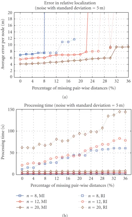
The majorization algorithm was performed using both the MDSInit and RandInit approaches. After obtaining the relative coordinates, the inter-node distances were calculated and compared to the inter-node distances from the actual coordinates. The elapsed processing time was also logged. This was then repeated with an increasing percentage of missing pairwise distances. The distances were removed in the order of their magnitude, such that the largest distances are first removed, until the required level is reached. The number of random multiple restart allowed for RandInit is limited to 50, from which the solution with the lowest stress function value was selected. The results are shown in Figures3–6. It is worth noting that the scale on theY-axis of the figures have been adjusted in order to give a better visual comparison. Any off-the-chart points, with values beyond the maximum on theY-axis, are considered to be the point at which the corresponding percentages of missing distances become large enough to contribute to significant performance degradation.
Each data-point of the simulation results is obtained by averaging over 10 random geometrical configurations. This relatively small number of random trials contributed to the non-smoothness in the data, but this sufficiently illustrates the trend of relationship between the parameters. Figure 3 shows the result under ideal measurement conditions, while
Figure 4shows the result where the distances are corrupted
with Gaussian noise of zero mean and 5 m standard deviation. Both the MDSInit and RandInit approaches are shown to have comparable minimization performance in terms of error from the actual distances, while the MDSInit approach has a lower tolerance to incomplete pairwise distances. Where the distances are corrupted by Gaussian noise (Figure 4(a)), the error performance is dominated by the noise, demonstrating that the error performance is very similar in both approaches. The spikes in the error charts are due to a node’s coordinate being resolved inaccurately, hence biasing the average error. As the missing pairwise measurements are those with the furthest distances, this occurred in the random arrangements where a single node was located much further away than the rest of the nodes, hence sharing most of the missing distances. This is verified by the results in Figure 5 obtained using ideal distance measurements, but with distances set to missing in a random manner as opposed to the largest distances. When missing distances are set as missing in a random manner, there is a smaller probability that any one node would suffer a much higher loss of measurements, hence the higher missing pairwise tolerances in both the approaches.
0 4 8 12 16 20 24 28 32 36 Percentage of missing pair-wise distances (%) 0
0.5 1 1.5 2 2.5 3 3.5 4 4.5 5 ×10⁻³
Av
er
ag
e
er
ro
r
p
er
n
o
d
e
(m
)
Error in relative localization (ideal measurement)
(a)
0 4 8 12 16 20 24 28 32 36
Percentage of missing pair-wise distances (%) 0
20 40 60 80 100 120 140
P
roc
essing
time
(s)
Processing time (ideal measurement)
n=8, MI
n=12, MI
n=20, MI
n=8, RI
n=12, RI
n=20, RI (b)
Figure 3: (a) Error performance; (b) processing time versus percentage of missing pairwise distances (where the larger distances are made missing) using ideally measured distances.
of multiple restarts was reduced to 15, the empirical level at which both the error performance and missing pairwise tolerance is comparable, the processing times were reduced to a level of up to 3 times longer.
5. Acoustic Field Trial
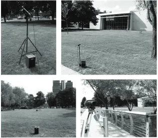
A practical demonstration of the localisation capabilities of a partially interconnected set of sensors was conducted during June 2009. A blustery, humid day was deliberately chosen to provide anisotropic propagation velocity conditions. The sensors were located on an undulating site to provide a 3D topography. This site was chosen to be adjacent to a road and under an airport flight path in order to provide intermittent noise conditions. Finally, high buildings surrounded two sides of the site in order to provide extreme multipath propagation conditions. Photographs of the site and equipment setup are shown inFigure 7.
Twelve microphones were located at positions previously determined using a survey-grade, carrier-phase-tracking
0 4 8 12 16 20 24 28 32 36
Percentage of missing pair-wise distances (%) 0
2 4 6 8 10 12 14 16 18 20
Av
er
ag
e
er
ro
r
p
er
n
o
d
e
(m
)
Error in relative localization (noise with standard deviation=5 m)
(a)
0 4 8 12 16 20 24 28 32 36
Percentage of missing pair-wise distances (%) 0
50 100 150
P
roc
essing
time
(s)
Processing time (noise with standard deviation=5 m)
n=8, MI
n=12, MI
n=20, MI
n=8, RI
n=12, RI
n=20, RI (b)
Figure 4: (a) Error performance; (b) processing time versus percentage of missing pairwise distances using distances with added 0 mean and 5 m standard deviation Gaussian noise.
global positioning satellites (GPS) receiver, as shown in Figure 8. Five of these microphones were colocated with a projector, whilst a roving projector was manually moved to the remaining seven microphone positions. Each projector was sequentially excited by a Hann weighted, linear fre-quency modulated sinusoid sweeping the band from 0 Hz to 16 kHz in 5.26 seconds. The receiver consisted of a bilaterally weighted matched filter providing a processing gain of some 46 dB against white noise. However, the coloured traffi c-noise environment and blustery conditions typically resulted in a processing gain varying from 20 to 35 dB.
A constant probability of false alarm (CFAR) detector
[45, 46] was used to automatically detect the occurrence
0 4 8 12 16 20 24 28 32 36 Percentage of missing pair-wise distances (%) 0
0.5 1 1.5 2 2.5 3 3.5 4 4.5 5 ×10⁻³
Av
er
ag
e
er
ro
r
p
er
n
o
d
e
(m
)
Error performance (random missing distances)
(a)
0 4 8 12 16 20 24 28 32 36
Percentage of missing pair-wise distances (%) 0
20 40 60 80 100 120
P
roc
essing
time
(s)
Processing time (random missing distances)
n=8, MI
n=12, MI
n=20, MI
n=8, RI
n=12, RI
n=20, RI (b)
Figure 5: (a) Error performance; (b) processing time versus percentage of missing pairwise distances using ideal distances, where the missing distances are randomly selected.
reverberation from the adjacent buildings and that the reverberation decays as an inverse square law. This is often associated with the adverse propagation conditions in the vicinity of the air-ground interface resulting from wind-shear and thermal profiles and unpredictable phase-changes [47]. A dynamic range of received signal strength in excess of 60 dB was encountered during the experiment.
Both the microphones and projectors have dimensions that are large in terms of wavelengths at the higher operating frequencies and thus become directional. The identification of the direct blast becomes virtually impossible under noise-and reverberation-limited conditions, resulting in a rnoise-andom selection of a multipath, as shown inFigure 10.
Under such circumstances, the approach adopted was to determine the cumulative distribution function and to place more confidence in results with tightly clustered distribu-tions. The zero-mean range estimate ensemble average of the cumulative distribution functions from fifty six available sensor pairs is illustrated inFigure 11. The limit of the shaded area equates to one standard deviation from the mean. It will
0 4 8 12 16 20 24 28 32 36
Percentage of missing pair-wise distances (%) 0
0.5 1 1.5 2 2.5 3 3.5 4 4.5 5 ×10⁻³
Av
er
ag
e
er
ro
r
p
er
n
o
d
e
(m
)
Error performance (less random restarts)
(a)
0 4 8 12 16 20 24 28 32 36
Percentage of missing pair-wise distances (%) 0
5 10 15 20 25 30 35 40 45 50 55
P
roc
essing
time
(s)
Processing time (less random restarts)
n=8, MI
n=12, MI
n=20, MI
n=8, RI
n=12, RI
n=20, RI (b)
Figure 6: (a) Error performance; (b) processing time with the number of multiple restart is constrained to 15, an empirical level at which both the error and missing distance tolerance performances are comparable for both approaches.
be noted that the standard deviation of the majority of range estimates is less than 1 m. With a temperature of 22◦C, the wind-free sound velocity is estimated as 345 ms−1.
The standard deviation of the range estimates may be used to compute a scoring matrix for use within the MDS algorithm, as shown inFigure 12. The value of the scoring matrix is calculated from 1−σr/σr, whereσrandσrrepresent
the standard deviation of a sensor pair range estimate and the peak standard deviation of all the sensor pair range estimates, respectively. Values of unity are associated with sensor-pairs with a low standard deviation. Where a higher value of standard deviation is encountered, or associated with the random selection of a multipath, a low score is returned and this measurement has less impact on the position estimation algorithm.
Figure7: The experimental site and the equipment setup on the site.
10 20 30 40 50 60
North (m) Building wall 45
40 35 30 25 20 15 10 5
East
(m)
Actual node positions as surveyed by carrier-phase tracking GPS
−60 −40 −20 0 20 40 60 80 100 120 140
(cm)
7 6
12 4
5 2
11 1
3 8
Trees 10
9
Figure 8: The actual positions of the nodes as surveyed by the carrier-phase tracking. GPS with regard to a local reference point. The contours depict the varying height of the site.
vectors derived from sensor pair measurements is shown in Figure 13. The centre of each cluster of vectors corresponds to the microphone position. The average length of the vectors varies significantly across the site because some microphones were nestling in hollows and were well shielded from the wind, whilst others were mounted on stands of typical height 1 m and placed in positions exposed to prevailing wind conditions.
The averaged wind speed across the sensor field was estimated as 1.94 m/s (7 km/hr) and a heading of 160 degrees. This compares with the meteorological wind speed measured
0 0.05 0.1 0.15 0.2 0.25 Time (s)
−140 −130 −120 −110 −100 −90 −80 −70 −60
M
ag
nitude
(dB
re
1
V
)
Detection
Cross correlation function output
Figure9: Typical matched filter output.
on the day of 19 km/hr from the North East direction, obtained from the nearest weather station at an airport about 12 km away. Therefore, the wind speed on the experimental site varied due to local conditions such as the presence of urban landscapes. The wind speed estimate was obtained from the difference between the time-delay measurements in opposite directions, a method applicable only when using time-of-arrival measurements.
The estimated ranges formed a 12×12 distance matrix,
0 0.05 0.1 0.15 0.2 0.25 Time (s)
−140 −130 −120 −110 −100 −90 −80 −70 −60
M
ag
nitude
(dB
re
1
V
)
Detection Cross correlation function output
Figure10: Extreme noise- and reverberation limited conditions.
−5 −4 −3 −2 −1 0 1 2 3 4 5 Range (m)
0 0.2 0.4 0.6 0.8 1
CDF deviation across1 standard
shaded region Cumulative distribution function of range estimates
Figure 11: Cumulative distribution functions of all zero-mean range estimates.
1 2 3 4 5 6 7 8 9 10 11 12
Senso
r numbe
r
1 2 3 4 5 6
7 8
9 1011 12
Senso r numbe
r
0 0.5 1
A
p
plied
sc
o
re
Scoring matrix for sensor pairs
Figure12: Scoring matrix derived from standard deviation of range estimates.
−10 0 10 20 30 40 50 60 70 East (m)
−10 0 10 20 30 40 50 60 70
No
rt
h
(m
)
Estimated wind speed vectors
Figure13: Estimate of wind speed vectors.
the final results from the algorithms. The error-per-node was calculated by taking the average of the absolute difference between Dactual andDmaj. Both the RandInit and MDSInit algorithms as detailed in Sections3.3and3.4, respectively, were applied on the estimated ranges. The estimated ranges were first processed with a unity weighting matrix such that
wi j equals to 1 for available distance entries or 0 otherwise,
over an increasing percentage of missing pairwise distances, chosen from the larger distances. This was then repeated with randomly chosen missing pairwise distances. The results are shown in Figures14and15, respectively.
It can be observed that the results are comparable with the prediction from the simulation study. The error performance is dominated by external factors such as varying wind conditions and the presence of bursty noise associated with the traffic. Therefore, the error performances of both the RandInit and MDSInit approaches are almost identical. Where the missing distances are set with largest distances, the tolerance to the level of missing distances is significantly lower as the error from the furthest node increases the average error.
The data were then processed by using a nonuniform weighting matrix that was scored in an inversely proportional manner to the standard deviation of the measured data. The results are shown in Figures16and17.
0 10 20 30 Percentage of missing pair-wise distances (%) 0
1 2 3 4 5 6
Er
ro
r
p
er
node
(m)
Error performance
(uniform weihgting/largest distances missing)
(a)
0 10 20 30
Percentage of missing pair-wise distances (%) 0
20 40 60 80 100 120
P
roc
essing
time
(s)
Processing time
(uniform weighting/largest distances missing)
MDSInit RandInit
(b)
Figure 14: (a) Error performance; (b) processing time versus percentage of missing pairwise distances with uniform weighting and largest distances missing.
that the adjusted-weighting yields estimates that better fit the measured distances.Figure 19shows the individual errors of the pairwise distances with respect to the actual distances, highlighting the fact that the average error per node can be biased due to the failure to resolve the relative location of a small number of nodes in the cluster.
The average wind speed estimate, as shown inFigure 13, can be used to build a compensation matrix for the resolved distances. By using the matrix dot product, the variation in sound velocity experienced by the path between any pair of nodes can be calculated. Figure 20 shows that the error from the actual distances is reduced when the velocity compensation matrix is applied based upon the average value of 1.94 m/s with a 160 degree heading. Both were processed with the MDSInit approach using adjusted weighting. Where all distance measurements are available, the average error per node from actual, GPS-surveyed, distances is 0.2 m. It is worth noting that the GPS survey
0 10 20 30
Percentage of missing pair-wise distances (%) 0.2
0.3 0.4 0.5 0.6 0.7 0.8 0.9 1 1.1 1.2
Er
ro
r
p
er
node
(m)
Error performance
(uniform weighting/random missing distances)
(a)
0 10 20 30
Percentage of missing pair-wise distances (%) 0
20 40 60 80 100 120
P
roc
essing
time
(s)
Processing time
(uniform weighting/random missing distances)
MDSInit RandInit
(b)
Figure 15: (a) Error performance; (b) processing time versus percentage of missing pairwise distances with uniform weighting and random missing distances.
data has a standard deviation of about 0.05 m, while the co-location of the projector and microphone has an ambiguity of approximately 0.03 m.
For completeness, the relative coordinates are mapped onto the reference coordinate shown in Figure 8. Three anchor points are chosen arbitrarily (nodes 1, 2, and 3) and the coordinate transformation matrix involving a 3-axes translation and a 3-axes rotation is derived using
Nelder-Mead minimization [48]. Figure 21 shows the mapped
coordinates of the nodes for different percentages of missing largest distances.
6. Scope of Study
0 10 20 30 Percentage of missing pair-wise distances (%) 0
1 2 3 4 5 6 7 8
Er
ro
r
p
er
node
(m)
Error performance (weighted/largest distances missing)
(a)
0 10 20 30
Percentage of missing pair-wise distances (%) 0
20 40 60 80 100 120
P
roc
essing
time
(s)
Processing time (weighted/largest distances missing)
MDSInit RandInit
(b)
Figure 16: (a) Error performance; (b) processing time versus percentage of missing pairwise distances with standard-deviation adjusted weighting and largest distances missing.
in sound velocity using the estimated wind vector reduces the error between the estimated distances and the actual distances. Similarly, in underwater applications where the sound velocity profile is available, the refraction path can be estimated to produce an adjustment matrix for the estimated distances. Also, the actual distances between available anchor nodes can be used to evaluate the reliability of the measured distances. More involved research related to the area of optimising the fit between the estimated and actual distances using information from anchor points can be found in [49,50].
The relative-localization problem considered in this arti-cle is for a cluster of node, but the solution is not necessarily restricted to a single-hop cluster. In a distributed, multi-hop arrangement of underwater nodes, relative-localization is usually reduced to the local positioning of a cluster of nodes with local anchor points, before iteratively optimizing the relative positions between the clusters. Therefore, the incomplete pairwise distance matrix can be considered as an
0 10 20 30
Percentage of missing pair-wise distances (%) 0.2
0.3 0.4 0.5 0.6 0.7 0.8 0.9 1 1.1 1.2
Er
ro
r
p
er
node
(m)
Error performance (weighted/random missing distances)
(a)
0 10 20 30
Percentage of missing pair-wise distances (%) 0
20 40 60 80 100 120
P
roc
essing
time
(s)
Processing time
(weighted/random missing distances)
MDSInit RandInit
(b)
Figure 17: (a) Error performance; (b) processing time versus percentage of missing pairwise distances with standard-deviation adjusted weighting and random missing distances.
0 10 20 30
Percentage of missing pair-wise distances (%) 20
40 60 80 100 120 140 160 180
St
re
ss
val
u
e
Stress values
Uniform weighting Adjusted weighting
1 2 3 4 5 6 7 8 9 10 11 12
No de
12 34
56 7 89 10
1112
Node
0 2 4 6 8 10 12
Individual errors (no distances missing)
(a)
1 2 3 4 5 6 7 8 9 10 11 12
No de
12 34
56 78
910 1112
Node
0 2 4 6 8 10 12
Individual errors (20% largest distances missing)
(b)
1 2 3 4 5 6 7 8 9 10 11 12
No de
1 2 3 4 5 6 7
8 9 10 11 12
Node
0 2 4 6 8 10 12
Individual errors (20% random missing distances)
(c)
Figure19: Individual error performances obtained with the MDSInit approach with adjusted weightings for (a) no missing distances, (b) 20% largest distances missing, and (c) 20% random missing distances.
irreducible matrix from a larger, global distance matrix for a distributed network of nodes.
A theoretical analysis on the performance constraints of relative location estimation as a function of the number of links to an anchor node and the total number of unanchored nodes is documented in [51].
Although the acoustic environment in which the exper-imental trial was conducted was also affected by ambient noise, multipath signal arrivals, and wind distortions, there are, nevertheless, notable differences from the underwater environment. The spectral characteristics of the ambient noise differ between the air-acoustic and the underwater environment. In the experiment, the main sources of ambi-ent noise were from the nearby traffic. In the underwater environment, the performance-limiting ambient noise may originate from various sources local shipping in coastal
waters, organisms such as snapping shrimps in tropical waters, and breaking waves. In both cases, the ambient noise would be expected to have non-stationary statistical characteristics. In terms of multipaths, reflections came from the buildings as well as the ground in the experimental environment, whilst in the underwater environment there are sea surface and sea bed reflections as well as multipaths from refractive spreading. The experimental environment is relatively homogeneous, and therefore gave rise to negligible refraction. The same is only valid in a very shallow water environment.
7. Conclusions
0 10 20 30 Percentage of missing pair-wise distances (%) 0
0.5 1 1.5 2 2.5 3 3.5 4 4.5
Av
er
ag
e
er
ro
r
p
er
n
o
d
e
(m
)
Error reduction from velocity compensation
With velocity compensation Without
Figure20: Reduction of error per node by velocity compensation using the average wind vector estimate.
10 20 30 40 50 60
North (m) 40
35 30 25 20 15 10 5
East
(m)
Mapped node positions
−60 −40 −20 0 20 40 60 80 100 120 140
(cm)
7 6
12 4
5 2
11 1
3 8
10 9
Figure21: Mapped node positions with respect to actual surveyed positions using anchor nodes 1, 2, and 3. Circles are actual surveyed positions, crosses are positions resolved with complete set of pair-wise distance, triangle are resolved with 10% largest distance miss-ing, while asterisks are resolved with 20% largest distance missing.
iterative majorization, which allows the estimation of relative coordinates using an incomplete pairwise distance matrix. An optimized initialization approach is proposed which demonstrated comparable minimization performance while requiring approximately 20 times less computing cycles.
It is shown that for underwater applications, sound refraction can contribute to the error between the measured and actual distances. However, in relatively shallow waters where the sound velocity gradient is benign and for ranges under 4000 m, the difference is likely to be small, but should be taken into account if the sound velocity profile is known.
Simulation study on the proposed approach demon-strated that the tolerance to missing pairwise distance is in the region of 8% to 30% depending on the number of nodes in the cluster and the pattern of missing distances. In cases where the missing pairwise distances are the largest distances, the tolerance is lower compared to randomly missing pairwise distances. This is because the higher loss of pairwise distances at the furthest nodes leads to failure to resolve their positions.
An acoustic field trial was carried out to evaluate the proposed algorithm. The results demonstrated that the application of a weighting function adjusted by the standard deviation of the observed data optimizes the fit between the estimated and measured distances, while the improvement in fit between the estimated and actual distances is much smaller. The estimated distances are then corrected using an estimate of the wind vector to calculate the variation from wind-free sound velocity during the trial. This leads to an observed reduction in the error of the estimated distances. The error performance and tolerance to missing pairwise distances of both approaches, as well as the significant reduction in processing time of the proposed approach are similarly demonstrated with the field trial measurements. Finally, the relative coordinates of the nodes are also mapped onto the reference coordinate of the site, showing good agreement with the actual nodes’ positions as surveyed by a carrier-phase-tracking GPS. Although both the simulation and experimental field trial results provided an indication to the practicality and robustness of the proposed algorithm in the context of optimising the process of relative positioning using incomplete distance measurements, it is worth noting that a direct extrapolation to predict its performance in an underwater environment is still constrained by variables that are not herein considered due the fundamental difference between the air-acoustic and the underwater environment.
Acknowledgments
The authors thank Mr. Zhaoyang You and Dr. Tim Collins for their contribution and assistance in the carrying out of the field trials.
References
[1] L. Freitag, M. Grund, S. Singh, and M. Johnson, “Acoustic communication in very shallow water: results from the 1999 AUV fest,” inProceedings of the IEEE Oceans Conference and Exhibition (OCEANS ’00), vol. 3, pp. 2155–2160, 2000. [2] D. B. Kilfoyle and A. B. Baggeroer, “The state of the art
in underwater acoustic telemetry,”IEEE Journal of Oceanic Engineering, vol. 25, no. 1, pp. 4–27, 2000.
[3] J. Heidemann, W. Ye, J. Wills, A. Syed, and L. Yuan, “Research challenges and applications for underwater sensor network-ing,” inProceedings of the IEEE Wireless Communications and Networking Conference (WCNC ’06), vol. 1, pp. 228–235, 2006. [4] G. Johnston, “Long term underwater positioning technologies for the offshore oil and gas industry,” inProceedings of IEEE Oceans Europe (OCEANS ’07), pp. 1–4, June 2007.
[5] E. M. Sozer, M. Stojanovic, and J. G. Proakis, “Underwater acoustic networks,”IEEE Journal of Oceanic Engineering, vol. 25, no. 1, pp. 72–83, 2000.
[6] J. Rice and D. Green, “Underwater acoustic communications and networks for the us navy’s seaweb program,” in Proceed-ings of the 2nd International Conference on Sensor Technologies and Applications, pp. 715–722, August 2008.
[8] J. Partan, J. Kurose, and B. N. Levine, “A survey of practical issues in underwater networks,”Mobile Computing and Com-munications Review, vol. 11, no. 4, pp. 23–33, 2007.
[9] M. Chitre, S. Shahabudeen, and M. Stojanovic, “Underwater acoustic communications and networking: recent advances and future challenges,”Marine Technology Society Journal, vol. 42, no. 1, pp. 103–116, 2008.
[10] J. de Leeuw and W. J. Heiser, “Convergence of correction matrix algorithms for multidimensional scaling,” in Data, Expert, Knowledge and Decisions, W. Gaul and M. Schader, Eds., pp. 329–340, Springer, Berlin, Germany, 1977.
[11] W. J. Heiser, “Convergent computation by iterative majoriza-tion: theory and applications in multidimensional data anal-ysis,” inRecent Advances in Descriptive Multivariate Analysis, W. J. Krzanowski, Ed., pp. 157–189, Oxford University Press, Oxford, UK, 1995.
[12] V. Chandrasekhar, W. K. G. Seah, Y. S. Choo, and H. V. Ee, “Localization in underwater sensor networks—survey and challenges,” inProceedings of the 1st ACM International Workshop on Underwater Networks (WUWNet ’06), vol. 2006, pp. 33–40, 2006.
[13] M. Chitre, J. Potter, and S. H. Ong, “Underwater acoustic channel characterisation for medium-range shallow water communications,” in Proceedings of the IEEE/MTS Oceans Conference, vol. 1, pp. 40–45, November 2004.
[14] D. E. Weston, A. A. Horrigan, S. J. L. Thomas, and J. Revie, “Studies of sound transmission fluctuations in shallow coastal water,” Philosophical Transactions for the Royal Society of London. Series A, vol. 265, no. 1169, pp. 567–606, 1969. [15] C. Eckart and G. Young, “The approximation of one matrix by
another of lower rank,”Psychometrika, vol. 1, no. 3, pp. 211– 218, 1936.
[16] W. S. Torgerson, “Multidimensional scaling: theory and method,”Psychometrika, vol. 17, pp. 401–419, 1952.
[17] Y. Shang, W. Ruml, Y. Zhang, and M. P. J. Fromherz, “Localization from mere connectivity,” inProceedings of the 4th International Symposium on Mobile Ad Hoc Networking and Computing (MobiHoc ’03), pp. 201–212, June 2003. [18] J. De Leeuw, “Convergence of the majorization method for
multidimensional scaling,”Journal of Classification, vol. 5, no. 2, pp. 163–180, 1988.
[19] P. J. F. Groenen,The Majorization Approach to Multidimen-sional Scaling: Some Problems and Extensions, DSWO Press, Leiden, The Netherlands, 1993.
[20] N. Bulusu, J. Heidemann, and D. Estrin, “GPS-less low-cost outdoor localization for very small devices,” IEEE Personal Communications Magazine, vol. 7, no. 5, pp. 28–34, 2000. [21] C. Savarese, J. Rabaey, and J. Beutel, “Locationing in
dis-tributed ad-hoc wireless sensor networks,” inProceedings of the IEEE International Conference on Acoustics, Speech and Signal Processing (ICASSP ’01), vol. 4, pp. 2037–2040, Salt Lake City, Utah, USA, 2001.
[22] R. L. Moses, D. Krishnamurthy, and R. M. Patterson, “A self-localization method for wireless sensor networks,”EURASIP Journal on Applied Signal Processing, vol. 2003, no. 4, pp. 348– 358, 2003.
[23] N. Patwari, A. O. Hero III, M. Perkins, N. Correal, and R. J. O’Dea, “Relative location estimation in wireless sensor networks,”IEEE Transactions on Signal Processing, vol. 51, no. 8, pp. 2137–2148, 2003.
[24] K. W. Cheung and H. C. So, “A multidimensional scaling framework for mobile location using time-of-arrival measure-ments,”IEEE Transactions on Signal Processing, vol. 53, no. 2, pp. 460–470, 2005.
[25] J. E. Garcia, “Ad hoc positioning for sensors in underwater acoustic networks,” inProceedings of the MTS/IEEE Oceans Conference (OCEANS ’04), vol. 4, pp. 2338–2340, November 2004.
[26] Z. Zhou, J.-H. Cui, and S. Zhou, “Localization for large-scale underwater sensor networks,” Tech. Rep. UbiNet-TR06-04, University of Connecticut, Computer Science and Engineer-ing, Storrs, Conn, USA, 2006.
[27] V. Chandrasekhar and W. Seah, “An area localization scheme for underwater sensor networks,” in Proceedings of the MTS/IEEE Oceans Conference (OCEANS ’06), pp. 1–8, May 2007.
[28] W. Cheng, A. Y. Teymorian, M. Liran, X. Cheng, X. Lu, and Z. Lu, “Underwater localization in sparse 3D acoustic sensor networks,” inProceedings of the 27th Conference on Computer Communications (INFOCOM ’08), pp. 236–240, April 2008. [29] M. Erol, L. Vieira, A. Caruso, F. Paparella, M. Gerla, and
S. Oktug, “Multi stage underwater sensor localization using mobile beacons,” in Proceedings of the 2nd International Conference on Sensor Technologies and Applications, (SENSOR-COMM ’08), pp. 710–714, August 2008.
[30] C. Wang and L. Xiao, “Sensor localization under limited measurement capabilities,”IEEE Network, vol. 21, no. 3, pp. 16–23, 2007.
[31] C. Knapp and G. C. Carter, “The generalized correlation method for estimation of time delay,”IEEE Transactions on Acoustics, Speech, and Signal Processing, vol. 24, no. 4, pp. 320– 327, 1976.
[32] X. Ji and H. Zha, “Sensor positioning in wireless ad-hoc sensor networks using multidimensional scaling,” inProceedings of the 23rd Annual Joint Conference of the IEEE Computer and Communications Societies (INFOCOM ’04), vol. 4, pp. 2652– 2661, 2004.
[33] J. A. Costa, N. Patwari, and A. O. Hero III, “Distributed weighted-multidimensional scaling for node localization in sensor networks,”ACM Transactions on Sensor Networks, vol. 2, no. 1, pp. 39–64, 2006.
[34] Y. M. Kwon, K. Mechitov, S. Sundresh, W. Kim, and G. Agha, “Resilient localization for sensor networks in outdoor envi-ronments,” inProceedings of the 25th International Conference on Distributed Computing Systems (ICSCS ’05), pp. 643–652, June 2005.
[35] S. T. Birchfield, “Geometric microphone array calibration by multidimensional scaling,” inProceedings of the IEEE Inter-national Conference on Acoustics, Speech and Signal Processing (ICASSP ’03), vol. 5, pp. 157–160, April 2003.
[36] I. Borg and P. J. F. Groenen,Modern Multidimensional Scaling: Theory and Applications, Springer Series in Statistics, Springer, London, UK, 2005.
[37] R. Fletcher, Practical Methods of Optimization, Wiley-Interscience, New York, NY, USA, 1987.
[38] K. Y. Foo, P. R. Atkins, S. A. Pointer, and C. P. Tiltman, “Robust time-division channel access approach for an ad hoc underwater network,” inProceedings of the 155th Meeting of the Acoustical Society of America, vol. 4, July 2008.
[39] A. K. Othman, “GPS-less localization protocol for underwater acoustic networks,” in Proceedings of the 5th International Conference on Wireless and Optical Communications Networks (WOCN ’08), pp. 1–6, May 2008.
[41] J. Shlens, “A tutorial on principal component analysis,” Tutorial, Center for Neural Science, New York University, New York, NY, USA, 2009, http://www.snl.salk.edu/∼shlens/pca .pdf.
[42] M. Schroeder,Springer Handbook of Acoustics, T. D. Rossing, Ed., Springer, London, UK, 2007.
[43] R. J. Urick, Principles of Underwater Sound for Engineers, McGraw-Hill, New York, NY, USA, 1975.
[44] C. R. Berger, S. Zhou, P. Willett, and L. Liu, “Stratification effect compensation for improved underwater acoustic rang-ing,”IEEE Transactions on Signal Processing, vol. 56, no. 8, pp. 3779–3783, 2008.
[45] V. G. Hansen and H. R. Ward, “Detection performance of the cell averaging LOG/CFAR receiver,”IEEE Transactions on Aerospace and Electronic Systems, vol. 8, no. 5, pp. 648–652, 1972.
[46] R. Nitzberg, “Analysis of the arithmetic mean CFAR normal-izer for fluctuating targets,” IEEE Transactions on Aerospace and Electronic Systems, vol. 14, no. 1, pp. 44–47, 1978. [47] U. J. Kurze and L. L. Beranek, “Sound propagation outdoors,”
inNoise and Vibration Control, L. L. Beranek, Ed., chapter 7, Institute of Noise Control Engineering, Washington, DC, USA, 1988.
[48] J. A. Nelder and R. Mead, “A simplex method for function minimization,”Computer Journal, vol. 7, pp. 308–313, 1965. [49] Y. T. Chan and K. C. Ho, “A simple and efficient estimator for
hyperbolic location,”IEEE Transactions on Signal Processing, vol. 42, no. 8, pp. 1905–1915, 1994.
[50] P.-C. Chen, “A non line-of-sight error mitigation algorithm in location estimation,” in Proceedings of the IEEE Wireless Communications and Networking Conference, vol. 1, pp. 316– 320, September 1999.