Learning Latent Tree Graphical Models

Learning Latent Tree Graphical Models

Myung Jin Choi [email protected]

Stochastic Systems Group

Laboratory for Information and Decision Systems Massachusetts Institute of Technology

Cambridge, MA 02139

Vincent Y. F. Tan [email protected]

Department of Electrical and Computer Engineering University of Wisconsin-Madison

Madison, WI 53706

Animashree Anandkumar [email protected]

Center for Pervasive Communications and Computing Electrical Engineering and Computer Science University of California, Irvine

Irvine, CA 92697

Alan S. Willsky [email protected]

Stochastic Systems Group

Laboratory for Information and Decision Systems Massachusetts Institute of Technology

Cambridge, MA 02139

Editor: Marina Meil˘a

Abstract

We study the problem of learning a latent tree graphical model where samples are available only from a subset of variables. We propose two consistent and computationally efficient algorithms for learning minimal latent trees, that is, trees without any redundant hidden nodes. Unlike many existing methods, the observed nodes (or variables) are not constrained to be leaf nodes. Our al-gorithms can be applied to both discrete and Gaussian random variables and our learned models are such that all the observed and latent variables have the same domain (state space). Our first algorithm, recursive grouping, builds the latent tree recursively by identifying sibling groups using so-called information distances. One of the main contributions of this work is our second algo-rithm, which we refer to as CLGrouping. CLGrouping starts with a pre-processing procedure in which a tree over the observed variables is constructed. This global step groups the observed nodes that are likely to be close to each other in the true latent tree, thereby guiding subsequent recursive grouping (or equivalent procedures such as neighbor-joining) on much smaller subsets of variables. This results in more accurate and efficient learning of latent trees. We also present regularized ver-sions of our algorithms that learn latent tree approximations of arbitrary distributions. We compare the proposed algorithms to other methods by performing extensive numerical experiments on var-ious latent tree graphical models such as hidden Markov models and star graphs. In addition, we demonstrate the applicability of our methods on real-world data sets by modeling the dependency structure of monthly stock returns in the S&P index and of the words in the 20 newsgroups data set.

1. Introduction

The inclusion of latent variables in modeling complex phenomena and data is a well-recognized and a valuable construct in a variety of applications, including bio-informatics and computer vision, and the investigation of machine-learning methods for models with latent variables is a substantial and continuing direction of research.

There are three challenging problems in learning a model with latent variables: learning the number of latent variables; inferring the structure of how these latent variables relate to each other and to the observed variables; and estimating the parameters characterizing those relationships. Is-sues that one must consider in developing a new learning algorithm include developing tractable methods; incorporating the tradeoff between the fidelity to the given data and generalizability; de-riving theoretical results on the performance of such algorithms; and studying applications that provide clear motivation and contexts for the models so learned.

One class of models that has received considerable attention in the literature is the class of latent

tree models, that is, graphical models Markov on trees, in which variables at some nodes represent

the original (observed) variables of interest while others represent the latent variables. The appeal of such models for computational tractability is clear: with a tree-structured model describing the statistical relationships, inference—processing noisy observations of some or all of the original variables to compute the estimates of all variables—is straightforward and scalable. Although the class of tree-structured models, with or without latent variables, is a constrained one, there are interesting applications that provide strong motivation for the work presented here. In particular, a very active avenue of research in computer vision is the use of context—for example, the nature of a scene to aid the reliable recognition of objects (and at the same time to allow the recognition of particular objects to assist in recognizing the scene). For example, if one knows that an image is that of an office, then one might expect to find a desk, a monitor on that desk, and perhaps a computer mouse. Hence if one builds a model with a latent variable representing that context (“office”) and uses simple, noisy detectors for different object types, one would expect that the detection of a desk would support the likelihood that one is looking at an office and through that enhance the reliability of detecting smaller objects (monitors, keyboards, mice, etc.). Work along these lines, including by some of the authors of this paper (Parikh and Chen, 2007; Choi et al., 2010), show the promise of using tree-based models of context.

This paper considers the problem of learning tree-structured latent models. If all variables are observed in the tree under consideration, then the well-known algorithm of Chow and Liu (1968) provides a tractable algorithm for performing maximum likelihood (ML) estimation of the tree structure. However, if not all variables are observed, that is, for latent tree models, then ML esti-mation is NP-hard (Roch, 2006). This has motivated a number of investigations of other tractable methods for learning such trees as well as theoretical guarantees on performance. Our work repre-sents a contribution to this area of investigation.

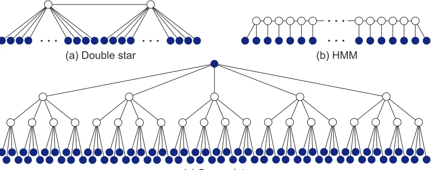
approach for a wide variety of models ranging from ones with very large tree diameters (e.g., hidden

Markov models (HMMs)) to star models and complete trees.1

Our first algorithm, which we refer to as recursive grouping, constructs a latent tree in a bottom-up fashion, grobottom-uping nodes into sibling grobottom-ups that share the same parent node, recursively at each level of the resulting hierarchy (and allowing for some of the observed variables to play roles at arbitrary levels in the resulting hierarchy). Our second algorithm, CLGrouping first implements a global construction step, namely producing the Chow-Liu tree for the observed variables without any hidden nodes. This global step then provides guidance for groups of observed nodes that are likely to be topologically close to each other in the latent tree, thereby guiding subsequent recursive grouping or neighbor-joining (Saitou and Nei, 1987) computations. Each of these algorithms is

consistent and has excellent sample and computational complexity.2

As Pearl (1988) points out, the identification of latent tree models has some built-in ambigu-ity, as there is an entire equivalence class of models in the sense that when all latent variables are marginalized out, each model in this class yields the same joint distribution over the observed vari-ables. For example, we can take any such latent model and add another hidden variable as a leaf node connected to only one other (hidden or observed) node. Hence, much as one finds in fields such as state space dynamic systems (e.g., Luenberger, 1979, Section 8), there is a notion of minimality that is required here, and our results are stated in terms of consistent learning of such minimal latent models.

1.1 Related Work

The relevant literature on learning latent models is vast and in this section, we summarize the main lines of research in this area.

The classical latent cluster models (LCM) consider multivariate distributions in which there exists only one latent variable and each state of that variable corresponds to a cluster in the data (Lazarsfeld and Henry, 1968). Hierarchical latent class (HLC) models (Zhang and Koˇcka, 2004; Zhang, 2004; Chen et al., 2008) generalize these models by allowing multiple latent variables. HLC allows latent variables to have different number of states, but assume that all observed nodes are at the leaves of the tree. Their learning algorithm is based on a greedy approach of making one local move at a time (e.g., introducing one hidden node, or replacing an edge), which is computationally expensive and does not have consistency guarantees. A greedy learning algorithm for HLC called BIN is proposed in Harmeling and Williams (2010), which is computationally more efficient. In addition, Silva et al. (2006) considered the learning of directed latent models using so-called tetrad constraints, and there have also been attempts to tailor the learning of latent tree models in order to perform approximate inference accurately and efficiently downstream (Wang et al., 2008). In all these works, the latent variables can have different state spaces, but the observed nodes are required to be leaves of the tree. In contrast, we fix the state space of each hidden node, but allow the possibility that some observed nodes are internal nodes (non-leaves). This assumption leads to an identifiable model, and we provide algorithms with consistency guarantees which can recover the correct structure under mild conditions. In contrast, the works in Zhang and Koˇcka (2004);

1. A tree is called a complete k-ary tree (or k-complete tree), if all its internal nodes have degree k and there exists one node (commonly referred as the root node) that has the exactly same distance to all leaf nodes.

Zhang (2004); Chen et al. (2008); Harmeling and Williams (2010) do not provide such consistency guarantees.

Many authors also propose reconstructing latent trees using the expectation maximization (EM) algorithm (Elidan and Friedman, 2005; Kemp and Tenenbaum, 2008). However, as with all other EM-based methods, these approaches depend on the initialization and suffer from the possibility of being trapped in local optima and thus no consistency guarantees can be provided. At each iteration, a large number of candidate structures need to be evaluated, so these methods assume that all observed nodes are the leaves of the tree to reduce the number of candidate structures. Algorithms have been proposed (Hsu et al., 2009) with sample complexity guarantees for learning HMMs under the condition that the joint distribution of the observed variables generated by distinct hidden states are distinct.

Another related line of research is that of (hierarchical) clustering. See Jain et al. (1999), Bal-can and Gupta (2010) and the references therein for extensive discussions. The primary objective of hierarchical clustering is to build a tree consisting of nested partitions of the observed data, where the leaves (typically) consist of single data points while the internal nodes represent coarser parti-tions. The difference from our work is that hierarchical clustering does not assume a probabilistic graphical model (Markov random field) on the data, but imposes constraints on the data points via a similarity matrix. We are interested in learning tree-structured graphical models with hidden variables.

The reconstruction of latent trees has been studied extensively by the phylogenetic community where sequences of extant species are available and the unknown phylogenetic tree is to be inferred from these sequences. See Durbin et al. (1999) for a thorough overview. Efficient algorithms with provable performance guarantees are available (Erd˝os et al., 1999; Daskalakis et al., 2006). However, the works in this area mostly assume that only the leaves are observed and each internal node (which is hidden) has the same degree except for the root. The most popular algorithm for constructing phylogenetic trees is the neighbor-joining (NJ) method by Saitou and Nei (1987). Like our recursive grouping algorithm, the input to the algorithm is a set of statistical distances between observed variables. The algorithm proceeds by recursively pairing two nodes that are the closest neighbors in the true latent tree and introducing a hidden node as the parent of the two nodes. For more details on NJ, the reader is referred to Durbin et al. (1999, Section 7.3).

Another popular class of reconstruction methods used in the phylogenetic community is the family of quartet-based distance methods (Bandelth and Dress, 1986; Erd˝os et al., 1999; Jiang

et al., 2001).3Quartet-based methods first construct a set of quartets for all subsets of four observed

nodes. Subsequently, these quartets are then combined to form a latent tree. However, when we only have access to the samples at the observed nodes, then it is not straightforward to construct a

latent tree from a set of quartets since the quartets may be not be consistent.4 In fact, it is known

that the problem of determining a latent tree that agrees with the maximum number of quartets is NP-hard (Steel, 1992), but many heuristics have been proposed (Farris, 1972; Sattath and Tversky, 1977). Also, in practice, quartet-based methods are usually much less accurate than NJ (St. John et al., 2003), and hence, we only compare our proposed algorithms to NJ in our experiments. For further comparisons (the sample complexity and other aspects of) between the quartet methods and NJ, the reader is referred to Cs˝ur¨os (2000) and St. John et al. (2003).

3. A quartet is simply an unrooted binary tree on a set of four observed nodes.

Another distance-based algorithm was proposed in Pearl (1988, Section 8.3.3). This algorithm is very similar in spirit to quartet-based methods but instead of finding quartets for all subsets of four observed nodes, it finds just enough quartets to determine the location of each observed node in the tree. Although the algorithm is consistent, it performs poorly when only the samples of observed nodes are available (Pearl, 1988, Section 8.3.5).

The learning of phylogenetic trees is related to the emerging field of network tomography (Cas-tro et al., 2004) in which one seeks to learn characteristics (such as structure) from data which are only available at the end points (e.g., sources and sinks) of the network. However, again observations are only available at the leaf nodes and usually the objective is to estimate the delay distributions corresponding to nodes linked by an edge (Tsang et al., 2003; Bhamidi et al., 2009). The modeling of the delay distributions is different from the learning of latent tree graphical models discussed in this paper.

1.2 Paper Organization

The rest of the paper is organized as follows. In Section 2, we introduce the notations and termi-nologies used in the paper. In Section 3, we introduce the notion of information distances which are used to reconstruct tree models. In the subsequent two sections, we make two assumptions: Firstly, the true distribution is a latent tree and secondly, perfect knowledge of information distance of observed variables is available. We introduce recursive grouping in Section 4. This is followed by our second algorithm CLGrouping in Section 5. In Section 6, we relax the assumption that the information distances are known and develop sample based algorithms and at the same time provide sample complexity guarantees for recursive grouping and CLGrouping. We also discuss extensions of our algorithms for the case when the underlying model is not a tree and our goal is to learn an approximation to it using a latent tree model. We demonstrate the empirical performance of our algorithms in Section 7 and conclude the paper in Section 8. The appendix includes proofs for the theorems presented in the paper.

2. Latent Tree Graphical Models

In this section, we provide some background and introduce the notion of minimal-tree extensions and consistency.

2.1 Undirected Graphs

Let G= (W,E) be an undirected graph with vertex (or node) set W =_{1, . . . ,M_} and edge set

E_⊂ W₂. Let nbd(i; G)and nbd[i; G]be the set of neighbors of node i and the closed neighborhood

of i respectively, that is, nbd[i; G]:=nbd(i; G)_{∪ {}i_}. If an undirected graph does not include any

loops, it is called a tree. A collection of disconnected trees is called a forest.5For a tree T= (W,E),

the set of leaf nodes (nodes with degree 1), the maximum degree, and the diameter are denoted by

Leaf(T),∆(T), and diam(T)respectively. The path between two nodes i and j in a tree T= (W,E),

which is unique, is the set of edges connecting i and j and is denoted as Path((i,j); E). The distance

between any two nodes i and j is the number of edges in Path((i,j); E). In an undirected tree, we

can choose a root node arbitrarily, and define the parent-child relationships with respect to the root:

for a pair neighboring nodes i and j, if i is closer to the root than j is, then i is called the parent of

j, and j is called the child of i. Note that the root node does not have any parent, and for all other

nodes in the tree, there exists exactly one parent. We use

C

of nodes that share the same parent is called a sibling group. A family is the union of the siblings and the associated parent.

A latent tree is a tree with node set W :=V_∪H, the union of a set of observed nodes V (with

m=_|V_|), and a set of latent (or hidden) nodes H. The effective depthδ(T ;V)(with respect to V ) is

the maximum distance of a hidden node to its closest observed node, that is, δ(T ;V):=max

i∈H minj∈V |Path((i,j); T)|. (1)

2.2 Graphical Models

An undirected graphical model (Lauritzen, 1996) is a family of multivariate probability distributions

that factorize according to a graph G= (W,E). More precisely, let X= (X1, . . . ,XM)be a random

vector, where each random variable Xi, which takes on values in an alphabet

X

vari-able at node i_∈V . The set of edges E encodes the set of conditional independencies in the model.

The random vector X is said to be Markov on G if for every i, the random variable Xiis conditionally

independent of all other variables given its neighbors, that is, if p is the joint distribution6of X, then

p(xi|xnbd(i;G)) =p(xi|x_\i), (2)

where x_\idenotes the set of all variables7excluding xi. Equation (2) is known as the local Markov

property.

In this paper, we consider both discrete and Gaussian graphical models. For discrete models,

the alphabet

X

X

without loss of generality, we assume that the mean is known to be the zero vector and hence, the joint distribution

p(x) = 1

det(2πΣ)1/2exp

−1

2x

T_Σ−1_x

depends only on the covariance matrixΣ.

An important and tractable class of graphical models is the set of tree-structured graphical

mod-els, that is, multivariate probability distributions that are Markov on an undirected tree T = (W,E).

It is known from junction tree theory (Cowell et al., 1999) that the joint distribution p for such a model factorizes as

p(x1, . . . ,xM) =

∏

p(xi)

∏

(i,j)∈E

p(xi,xj)

p(xi)p(xj)

. (3)

That is, the sets of marginal_{p(xi): i∈W}and pairwise joints on the edges{p(xi,xj):(i,j)∈E}

fully characterize the joint distribution of a tree-structured graphical model.

A special class of a discrete tree-structured graphical models is the set of symmetric discrete

distributions. This class of models is characterized by the fact that the pairs of variables(Xi,Xj)on

6. We abuse the term distribution to mean a probability mass function in the discrete case (density with respect to the counting measure) and a probability density function (density with respect to the Lebesgue measure) in the continuous case.

all the edges(i,j)_∈E follow the conditional probability law:

p(xi|xj) =

1₋(K₋1)θi j, if xi=xj,

θi j, otherwise, (4)

and the marginal distribution of every variable in the tree is uniform, that is, p(xi) =1/K for all

xi ∈

X

state values xi,xj∈

X

probability.

Let xn_:={x(1)_{, . . . ,x}(n)_{}be a set of n i.i.d. samples drawn from a graphical model (distribution)}

p, Markov on a latent tree Tp= (W,Ep), where W =V∪H. Each sample x(l)∈

X

vector. In our setup, the learner only has access to samples drawn from the observed node set V , and

we denote this set of sub-vectors containing only the elements in V , as x_Vn :=_{x_V(1), . . . ,x_V(n)_}, where

each observed sample x_V(l)_∈

X

using the information distances (defined in Section 3) between pairs of observed variables, which can be estimated from samples.

We now comment on the above model assumptions. Note that we assume that the the hidden variables have the same domain as the observed ones (all of which also have a common domain). We do not view this as a serious modeling restriction since we develop efficient algorithms with strong theoretical guarantees, and these algorithms have very good performance on real-world data (see Section 7). Nonetheless, it may be possible to develop a unified framework to incorporate variables with different state spaces (i.e., both continuous and discrete) under a reproducing kernel Hilbert space (RKHS) framework along the lines of Song et al. (2010). We defer this to future work.

2.3 Minimal Tree Extensions

Our ultimate goal is to recover the graphical model p, that is, the latent tree structure and its

param-eters, given n i.i.d. samples of the observed variables xn_V. However, in general, there can be multiple

latent tree models which result in the same observed statistics, that is, the same joint distribution pV

of the observed variables. We consider the class of tree models where it is possible to recover the latent tree model uniquely and provide necessary conditions for structure identifiability, that is, the identifiability of the edge set E.

Firstly, we limit ourselves to the scenario where all the random variables (both observed and

latent) take values on a common alphabet

X

variable is a univariate Gaussian. In the discrete case, each variable takes on values in the same

finite alphabet

X

allowed to have arbitrary alphabets. As an example, consider a discrete latent tree model with binary

observed variables (K=2). A latent tree with the simplest structure (fewest number of nodes) is a

tree in which all m observed binary variables are connected to one hidden variable. If we allow the

hidden variable to take on 2mstates, then the tree can describe all possible statistics among the m

observed variables, that is, the joint distribution pV can be arbitrary.8

A probability distribution pV(xV)is said to be tree-decomposable if it is the marginal (of

vari-ables in V ) of a tree-structured graphical model p(xV,xH). In this case, p (over variables in W ) is

said to be a tree extension of pV (Pearl, 1988). A distribution p is said to have a redundant

hid-den node h_∈H if we can remove h and the marginal on the set of visible nodes V remains as pV.

(a)

h1

1

2 3 4 5

6

h3

h2

(b)

h1

1

2 3 4 5

6

h3

h2

h5

h4

Figure 1: Examples of minimal latent trees. Shaded nodes are observed and unshaded nodes are

hidden. (a) An identifiable tree. (b) A non-identifiable tree because h4 and h5 have

degrees less than 3.

The following conditions ensure that a latent tree does not include a redundant hidden node (Pearl, 1988):

(C1) Each hidden variable has at least three neighbors (which can be either hidden or observed). Note that this ensures that all leaf nodes are observed (although not all observed nodes need to be leaves).

(C2) Any two variables connected by an edge in the tree model are neither perfectly dependent nor independent.

Figure 1(a) shows an example of a tree satisfying (C1). If (C2), which is a condition on param-eters, is also satisfied, then the tree in Figure 1(a) is identifiable. The tree shown in Figure 1(b) does

not satisfy (C1) because h4and h5have degrees less than 3. In fact, if we marginalize out the hidden

variables h4and h5, then the resulting model has the same tree structure as in Figure 1(a).

We assume throughout the paper that (C2) is satisfied for all probability distributions. Let

T

be the set of (latent) trees satisfying (C1). We refer to

T

latent trees. Minimal latent trees do not contain redundant hidden nodes. The distribution p (over W and Markov on some tree in

T

Figure 1, using marginalization operations, any non-minimal latent tree distribution can be reduced to a minimal latent tree model.

Proposition 1 (Minimal Tree Extensions) (Pearl, 1988, Section 8.3)

(i) For every tree-decomposable distribution pV, there exists a minimal tree extension p Markov

on a tree T_∈

T

p can be recovered.

2.4 Consistency

We now define the notion of consistency. In Section 6, we show that our latent tree learning algo-rithms are consistent.

Definition 2 (Consistency) A latent tree reconstruction algorithm

A

A

homo-morphism9h such that

lim

n→∞Pr(h(Tb

n_)6=T

p) =0. (5)

Furthermore, we say that

A

n→∞Pr(D(p||bp

n_{)>ε) =0, (6)}

where D(p_||p_bn) is the KL-divergence (Cover and Thomas, 2006) between the true distribution p and the estimated distribution_bpn.

In the following sections, we design structurally and risk consistent algorithms for (minimal) Gaussian and symmetric discrete latent tree models, defined in (4). Our algorithms use pairwise distributions between the observed nodes. However, for general discrete models, pairwise distribu-tions between observed nodes are, in general, not sufficient to recover the parameters (Chang and Hartigan, 1991). Therefore, we only prove structural consistency, as defined in (5), for general dis-crete latent tree models. For such distributions, we consider a two-step procedure for structure and parameter estimation: Firstly, we estimate the structure of the latent tree using the algorithms sug-gested in this paper. Subsequently, we use the Expectation Maximization (EM) algorithm (Dempster et al., 1977) to infer the parameters. Note that, as mentioned previously, risk consistency will not be guaranteed in this case.

3. Information Distances

The proposed algorithms in this paper receive as inputs the set of so-called (exact or estimated)

information distances, which are functions of the pairwise distributions. These quantities are defined

in Section 3.1 for the two classes of tree-structured graphical models discussed in this paper, namely the Gaussian and discrete graphical models. We also show that the information distances have a particularly simple form for symmetric discrete distributions. In Section 3.2, we use the information distances to infer the relationships between the observed variables such as j is a child of i or i and j are siblings.

3.1 Definitions of Information Distances

We define information distances for Gaussian and discrete distributions and show that these

dis-tances are additive for tree-structured graphical models. Recall that for two random variables Xiand

Xj, the correlation coefficient is defined as

ρi j:=

Cov(Xi,Xj)

p

Var(Xi)Var(Xj)

. (7)

9. A graph homomorphism is a mapping between graphs that respects their structure. More precisely, a graph homo-morphism h from a graph G= (W,E)to a graph G′= (V′,E′), written h : G→G′is a mapping h : V→V′such that

For Gaussian graphical models, the information distance associated with the pair of variables Xiand

Xj is defined as:

di j :=−log|ρi j|. (8)

Intuitively, if the information distance di j is large, then Xi and Xj are weakly correlated and

vice-versa.

For discrete random variables, let Ji jdenote the joint probability matrix between Xiand Xj(i.e.,

J_abi j =p(xi=a,xj=b),a,b∈

X

Mi_aa=p(xi=a)). For discrete graphical models, the information distance associated with the pair

of variables Xiand Xj is defined as Lake (1994):

di j:=−log |

det Ji j_|

√

det Mi_{det M}j. (9)

Note that for binary variables, that is, K=2, the value of di jin (9) reduces to the expression in (8),

that is, the information distance is a function of the correlation coefficient, defined in (7), just as in the Gaussian case.

For symmetric discrete distributions defined in (4), the information distance defined for discrete graphical models in (9) reduces to

di j:=−(K−1)log(1−Kθi j). (10)

Note that there is one-to-one correspondence between the information distances di j and the model

parameters for Gaussian distributions (parametrized by the correlation coefficientρi j) in (8) and the

symmetric discrete distributions (parametrized by the crossover probabilityθi j) in (10). Thus, these

two distributions are completely characterized by the information distances di j. On the other hand,

this does not hold for general discrete distributions.

Moreover, if the underlying distribution is a symmetric discrete model or a Gaussian model,

the information distance di j and the mutual information I(Xi; Xj) (Cover and Thomas, 2006) are

monotonic, and we will exploit this result in Section 5. For general distributions, this is not valid. See Section 5.5 for further discussions.

Equipped with these definitions of information distances, assumption (C2) in Section 2.3 can be

rewritten as the following: There exists constants 0<l,u<∞, such that

(C2) l_≤di j≤u, ∀(i,j)∈Ep. (11)

Proposition 3 (Additivity of Information Distances) The information distances di j defined in (8),

(9), and (10) are additive tree metrics (Erd˝os et al., 1999). In other words, if the joint probability distribution p(x) is a tree-structured graphical model Markov on the tree Tp= (W,Ep), then the

information distances are additive on Tp:

dkl=

∑

(i,j)∈Path((k,l);Ep)

di j, ∀k,l∈W. (12)

The property in (12) implies that if each pair of vertices i,j_∈W is assigned the weight di j, then

Tpis a minimum spanning tree on W , denoted as MST(W ; D), where D is the information distance

(a) (b) (c) (d) (e)

i

j

e1 _e 2 e3

e4 e5 e6 e7

e8

j

e1 _e 2 e3

e4 e5 e6 e7

e8

i j

e1 _e 2 e3

e4 e5 e6 e7

e8

i k

k `

j

e1 _e 2 e3

e4 e5 e6 e7

e8

i

k k `

j

e1 _e 2 e3

e4 e5 e6 e7

e8

i

k k `

Figure 2: Examples for each case in TestNodeRelationships. For each edge, ei represents the

information distance associated with the edge. (a) Case 1: Φi jk =−e8=−di j for all

k_∈V_{\ {}i,j_}. (b) Case 2:Φi jk=e6−e7=6 di j=e6+e7for all k∈V\ {i,j}(c) Case 3a:

Φi jk=e4+e2+e3−e76=Φi jk′=e4−e2−e3−e7. (d) Case 3b:Φi jk=e4+e56=Φi jk′=

e4−e5. (e) Case 3c:Φi jk=e56=Φi jk′=−e₅.

It is straightforward to show that the information distances are additive for the Gaussian and symmetric discrete cases using the local Markov property of graphical models. For general discrete distributions with information distance as in (9), see Lake (1994) for the proof. In the rest of the paper, we map the parameters of Gaussian and discrete distributions to an information distance

matrix D= [di j]to unify the analyses for both cases.

3.2 Testing Inter-Node Relationships

In this section, we use Proposition 3 to ascertain child-parent and sibling (cf., Section 2.1) relation-ships between the variables in a latent tree-structured graphical model. To do so, for any three

vari-ables i,j,k_∈V , we defineΦi jk:=dik−djk to be the difference between the information distances

dik and djk. The following lemma suggests a simple procedure to identify the set of relationships

between the nodes.

Lemma 4 (Sibling Grouping) For distances di j for all i,j∈V on a tree T ∈

T

(i) Φi jk=di jfor all k∈V\ {i,j}if and only if i is a leaf node and j is its parent.

(i) Φi jk=−di j for all k∈V\ {i,j}if and only if j is a leaf node and i is its parent.

(ii) ₋di j<Φi jk=Φi jk′<di jfor all k,k′∈V\ {i,j}if and only if both i and j are leaf nodes and

they have the same parent, that is, they belong to the same sibling group.

The proof of the lemma uses Proposition 3 and is provided in Appendix A.1. Given Lemma 4,

we can first determine all the values of Φi jk for triples i,j,k∈V . Now we can determine the

relationship between nodes i and j as follows: Fix the pair of nodes i,j_∈V and consider all the

other nodes k_∈V_{\ {}i,j_}. Then, there are three cases for the set_{Φi jk: k∈V\ {i,j}}:

1. Φi jk =di j for all k∈V\ {i,j}. Then, i is a leaf node and j is a parent of i. Similarly, if

Φi jk=−di j for all k∈V\ {i,j}, j is a leaf node and i is a parent of j.

2. Φi jk is constant for all k∈V\ {i,j}but not equal to either di j or−di j. Then i and j are leaf

3. Φi jkis not equal for all k∈V\ {i,j}. Then, there are three cases: Either

(a) Nodes i and j are not siblings nor have a parent-child relationship or, (b) Nodes i and j are siblings but at least one of them is not a leaf or, (c) Nodes i and j have a parent-child relationship but the child is not a leaf.

Thus, we have a simple test to determine the relationship between i and j and to ascertain whether i

and j are leaf nodes. We call the above testTestNodeRelationships. See Figure 2 for examples. By

running this test for all i and j, we can determine all the relationships among all pairs of observed variables.

In the following section, we describe a recursive algorithm that is based on the above TestNodeRelationshipsprocedure to reconstruct the entire latent tree model assuming that the true

model is a latent tree and that the true distance matrix D= [di j]are known. In Section 5, we provide

improved algorithms for the learning of latent trees again assuming that D is known. Subsequently, in Section 6, we develop algorithms for the consistent reconstruction of latent trees when

infor-mation distances are unknown and we have to estimate them from the samples xn_V. In addition,

in Section 6.6 we discuss how to extend these algorithms for the case when pV is not necessarily

tree-decomposable, that is, the original graphical model is not assumed to be a latent tree.

4. Recursive Grouping Algorithm Given Information Distances

This section is devoted to the development of the first algorithm for reconstructing latent tree mod-els, recursive grouping (RG). At a high level, RG is a recursive procedure in which at each step, TestNodeRelationshipsis used to identify nodes that belong to the same family. Subsequently, RG introduces a parent node if a family of nodes (i.e., a sibling group) does not contain an observed parent. This newly introduced parent node corresponds to a hidden node in the original unknown latent tree. Once such a parent (i.e., hidden) node h is introduced, the information distances from h to all other observed nodes can be computed.

The inputs to RG are the vertex set V and the matrix of information distances D corresponding to a latent tree. The algorithm proceeds by recursively grouping nodes and adding hidden variables. In each iteration, the algorithm acts on a so-called active set of nodes Y , and in the process constructs

a new active set Ynewfor the next iteration.10 The steps are as follows:

1. Initialize by setting Y :=V to be the set of observed variables.

2. ComputeΦi jk=dik−djkfor all i,j,k∈Y .

3. Using theTestNodeRelationshipsprocedure, define_{Πl}Ll=1to be the coarsest partition11of

Y such that for every subsetΠl(with|Πl| ≥2), any two nodes inΠl are either siblings which

10. Note that the current active set is also used (in Step 6) after the new active set has been defined. For clarity, we also introduce the quantity Yoldin Steps 5 and 6.

11. Recall that a partition P of a set Y is a collection of nonempty subsets{Πl⊂Y}L

l=1 such that∪

L

l=1Πl=Y and

are leaf nodes or they have a parent-child relationship12in which the child is a leaf.13 Note

that for some l, Πl may consist of a single node. Begin to construct the new active set by

adding nodes in these single-node partitions: Ynew←Sl:|Πl|=1Πl.

4. For each l=1, . . . ,L with_|Πl| ≥2, ifΠlcontains a parent node u, update Ynew←Ynew∪ {u}.

Otherwise, introduce a new hidden node h, connect h (as a parent) to every node inΠl, and

set Ynew←Ynew∪ {h}.

5. Update the active set: Yold←Y and Y ←Ynew.

6. For each new hidden node h_∈Y , compute the information distances dhlfor all l∈Y using (13)

and (14) described below.

7. If_|Y_{| ≥}3, return to step 2. Otherwise, if_|Y_|=2, connect the two remaining nodes in Y with

an edge then stop. If instead_|Y_|=1, do nothing and stop.

We now describe how to compute the information distances in Step 6 for each new hidden node

h_∈Y and all other active nodes l_∈Y . Let i,j_∈

C

be any other node in the previous active set. From Lemma 4 and Proposition 3, we have that

dih−djh=dik−djk=Φi jkand dih+djh=di j, from which we can recover the information distances

between a previously active node i_∈Yoldand its new hidden parent h∈Y as follows:

dih=

1

2 di j+Φi jk

. (13)

For any other active node l_∈Y , we can compute dhl using a child node i∈

C

dhl=

dil−dih, if l∈Yold,

dik−dih−dlk, otherwise, where k∈

C

(14)

Using Equations (13) and (14), we can infer all the information distances dhl between a newly

introduced hidden node h to all other active nodes l_∈Y . Consequently, we have all the distances

di j between all pairs of nodes in the active set Y . It can be shown that this algorithm recovers all

minimal latent trees. The proof of the following theorem is provided in Appendix A.2.

Theorem 5 (Correctness and Computational Complexity of RG) If Tp∈

T

correctly in time O(diam(Tp)m3).

We now use a concrete example to illustrate the steps involved in RG. In Figure 3(a), the original

unknown latent tree is shown. In this tree, nodes 1, . . . ,6 are the observed nodes and h1,h2,h3are the

hidden nodes. We start by considering the set of observed nodes as active nodes Y :=V=_{1, . . . ,6_}.

OnceΦi jkare computed from the given distances di j,TestNodeRelationshipsis used to determine

that Y is partitioned into four subsets:Π1={1},Π2={2,4},Π3={5,6},Π4={3}. The subsetsΠ1

12. In an undirected tree, the parent-child relationships can be defined with respect to a root node. In this case, the node in the final active set in Step 7 before the algorithm terminates (or one of the two final nodes if|Y|=2) is selected as the root node.

hh2 h3

1 2

4

3

5 6

h1

(a)

1 2

4

3

5 6

h1

(b) (c)

hh2 h3

1 2 h1 3

4 5 6

(d)

1 2 h1 3

4 5 6

h2 h3

Figure 3: An illustrative example of RG. Solid nodes indicate the active set Y for each iteration. (a) Original latent tree. (b) Output after the first iteration of RG. Red dotted lines indicate

the subsetsΠlin the partition of Y . (c) Output after the second iteration of RG. Note that

h3, which was introduced in the first iteration, is an active node for the second iteration.

Nodes 4,5, and 6 do not belong to the current active set and are represented in grey. (d) Output after the third iteration of RG, which is same as the original latent tree.

andΠ4contain only one node. The subsetΠ3contains two siblings that are leaf nodes. The subset

Π2contains a parent node 2 and a child node 4, which is a leaf node. SinceΠ3does not contain a

parent, we introduce a new hidden node h1and connect h1to 5 and 6 as shown in Figure 3(b). The

information distances d5h1 and d6h1can be computed using (13), for example, d5h1 =

1

2(d56+Φ561).

The new active set is the union of all nodes in the single-node subsets, a parent node, and a new

hidden node Ynew ={1,2,3,h1}. Distances among the pairs of nodes in Ynew can be computed

using (14) (e.g., d1h1 =d15−d5h1). In the second iteration, we again useTestNodeRelationships

to ascertain that Y can be partitioned intoΠ1={1,2}andΠ2={h1,3}. These two subsets do not

have parents so h2and h3are added toΠ1andΠ2respectively. Parent nodes h2and h3are connected

to their children inΠ1 andΠ2 as shown in Figure 3(c). Finally, we are left with the active set as

Y =_{h2,h3_}and the algorithm terminates after h2and h3 are connected by an edge. The hitherto

unknown latent tree is fully reconstructed as shown in Figure 3(d).

A potential drawback of RG is that it involves multiple local operations, which may result in

a high computational complexity. Indeed, from Theorem 5, the worst-case complexity is O(m4)

which occurs when Tp, the true latent tree, is a hidden Markov model (HMM). This may be

com-putationally prohibitive if m is large. In Section 5 we design an algorithm which uses a global pre-processing step to reduce the overall complexity substantially, especially for trees with large diameters (of which HMMs are extreme examples).

5. CLGrouping Algorithm Given Information Distances

obtain the latent tree in Section 5.3 and propose CLGrouping in Section 5.4. For simplicity, we focus on the Gaussian distributions and the symmetric discrete distributions first, and discuss the extension to general discrete models in Section 5.5.

5.1 A Review of the Chow-Liu Algorithm

In this section, we review the Chow-Liu tree reconstruction procedure. To do so, define

T

be the set of trees with vertex set V and

P

T

whose graph has vertex set V , that is, every q_∈

P

T

Given an arbitrary multivariate distribution pV(xV), Chow and Liu (1968) considered the

fol-lowing KL-divergence minimization problem:

pCL:= argmin

q_∈P(T(V))

D(pV||q). (15)

That is, among all the tree-structured graphical models with vertex set V , the distribution pCL is

the closest one to pV in terms of the KL-divergence. By using the factorization property in (3), we

can easily verify that pCL is Markov on the Chow-Liu tree TCL = (V,ECL)which is given by the

optimization problem:14

TCL=argmax

T_∈T(V) (i,

∑

I(Xi; Xj). (16)

In (16), I(Xi; Xj) =D(p(xi,xj)||p(xi)p(xj))is the mutual information (Cover and Thomas, 2006)

between random variables Xi and Xj. The optimization in (16) is a max-weight spanning tree

prob-lem (Cormen et al., 2003) which can be solved efficiently in time O(m2log m)using either Kruskal’s

algorithm (Kruskal, 1956) or Prim’s algorithm (Prim, 1957). The edge weights for the max-weight spanning tree are precisely the mutual information quantities between random variables. Note that

once the optimal tree TCLis formed, the parameters of pCLin (15) are found by setting the pairwise

distributions pCL(xi,xj)on the edges to pV(xi,xj), that is, pCL(xi,xj) =pV(xi,xj)for all(i,j)∈ECL.

We now relate the Chow-Liu tree on the observed nodes and the information distance matrix D.

Lemma 6 (Correspondence between TCLand MST) If pV is a Gaussian distribution or a

sym-metric discrete distribution, then the Chow-Liu tree in (16) reduces to the minimum spanning tree (MST) where the edge weights are the information distances di j, that is,

TCL=MST(V ; D):=argmin

T∈T(V) _(i,

∑

di j. (17)

Lemma 6, whose proof is omitted, follows because for Gaussian and symmetric discrete

mod-els, the mutual information15 I(Xi; Xj) is a monotonically decreasing function of the information

distance di j.16 For other graphical models (e.g., non-symmetric discrete distributions), this

relation-ship is not necessarily true. See Section 5.5 for a discussion. Note that when all nodes are observed

(i.e., W =V ), Lemma 6 reduces to Proposition 3.

14. In (16) and the rest of the paper, we adopt the following simplifying notation; If T= (V,E)and if(i,j)∈E, we will also say that(i,j)∈T .

15. Note that, unlike information distances di j, the mutual information quantities I(Xi; Xj)do not form an additive metric

on Tp.

5.2 Relationship between the Latent Tree and the Chow-Liu Tree (MST)

In this section, we relate MST(V ; D)in (17) to the original latent tree Tp. To relate the two trees,

MST(V ; D)and Tp, we first introduce the notion of a surrogate node.

Definition 7 (Surrogate Node) Given the latent tree Tp= (W,Ep)and any node i∈W , the

surro-gate node of i with respect to V is defined as

Sg(i; Tp,V):=argmin

j_∈V

di j.

Intuitively, the surrogate node of a hidden node h∈H is an observed node j∈V that is most

strongly correlated to h. In other words, the information distance between h and j is the smallest.

Note that if i_∈V , then Sg(i; Tp,V) =i since dii=0. The map Sg(i; Tp,V)is a many-to-one function,

that is, several nodes may have the same surrogate node, and its inverse is the inverse surrogate set

of i denoted as

Sg−1(i; Tp,V):={h∈W : Sg(h; Tp,V) =i}.

When the tree Tp and the observed vertex set V are understood from context, the surrogate node

of h and the inverse surrogate set of i are abbreviated as Sg(h)and Sg−1(i)respectively. We now

relate the original latent tree Tp= (W,Ep)to the Chow-Liu tree (also termed the MST) MST(V ; D)

formed using the distance matrix D.

Lemma 8 (Properties of the MST) The MST in (17) and surrogate nodes satisfy the following

properties:

(i) The surrogate nodes of any two neighboring nodes in Ep are neighbors in the MST, that is,

for all i,j_∈W with Sg(i)₆=Sg(j),

(i,j)_∈Ep⇒(Sg(i),Sg(j))∈MST(V ; D). (18)

(ii) If j_∈V and h_∈Sg−1(j), then every node along the path connecting j and h belongs to the inverse surrogate set Sg−1(j).

(iii) The maximum degree of the MST satisfies

∆(MST(V ; D))_≤∆(Tp)1+ u

lδ(Tp;V)_{, (19)}

whereδ(Tp;V)is the effective depth defined in (1) and l,u are the bounds on the information

distances on edges in Tpdefined in (11).

The proof of this result can be found in Appendix A.3. As a result of Lemma 8, the properties

of MST(V ; D)can be expressed in terms of the original latent tree Tp. For example, in Figure 5(a),

a latent tree is shown with its corresponding surrogacy relationships, and Figure 5(b) shows the corresponding MST over the observed nodes.

The properties in Lemma 8(i-ii) can also be regarded as edge-contraction operations (Robinson and Foulds, 1981) in the original latent tree to obtain the MST. More precisely, an edge-contraction

operation on an edge(j,h)_∈V_×H in the latent tree Tp is defined as the “shrinking” of(j,h)to

4 5 4 5

(a)

1

2 3

(b) (c) (d) (e) (f)

h1 h2

1 2 3 4 5

h2

1 2

3 4 5

2 3

1

h2

1 2

3 4 5

h1 h2

1 2 3 4 5

Figure 4: An illustration of CLBlind. The shaded nodes are the observed nodes and the rest are hidden nodes. The dotted lines denote surrogate mappings for the hidden nodes. (a) Original latent tree, which belongs to the class of blind latent graphical models, (b) Chow-Liu tree over the observed nodes, (c) Node 3 is the input to the blind transformation, (d) Output after the blind transformation, (e) Node 2 is the input to the blind transformation, (f) Output after the blind transformation, which is same as the original latent tree.

node j. By using Lemma 8(i-ii), we observe that the Chow-Liu tree MST(V ; D) is formed by

applying edge-contraction operations to each(j,h)pair for all h_∈Sg−1(j)_∩H sequentially until

all pairs have been contracted to a single node j. For example, the MST in Figure 5(b) is obtained

by contracting edges(3,h3),(5,h2), and then(5,h1)in the latent tree in Figure 5(a).

The properties in Lemma 8 can be used to design efficient algorithms based on transforming

the MST to obtain the latent tree Tp. Note that the maximum degree of the MST,∆(MST(V ; D)), is

bounded by the maximum degree in the original latent tree. The quantity∆(MST(V ; D))determines

the computational complexity of one of our proposed algorithms (CLGrouping) and it is small if the

depth of the latent treeδ(Tp;V)is small (e.g., HMMs) and the information distances di j satisfy tight

bounds (i.e., u/l is close to unity). The latter condition holds for (almost) homogeneous models in

which all the information distances di j on the edges are almost equal.

5.3 Chow-Liu Blind Algorithm for a Subclass of Latent Trees

In this section, we present a simple and intuitive transformation of the Chow-Liu tree that produces the original latent tree. However, this algorithm, called Chow-Liu Blind (or CLBlind), is

applica-ble only to a subset of latent trees called blind latent tree-structured graphical models

P

T

Equipped with the intuition from CLBlind, we generalize it in Section 5.4 to design the CLGroup-ing algorithm that produces the correct latent tree structure from the MST for all minimal latent tree models.

If p_∈

P

T

properties:

(i) The true latent tree Tp∈

T

(ii) The surrogate node of (i.e., the observed node with the strongest correlation with) each hidden

node is one of its children, that is, Sg(h)_∈

C

We now describe the CLBlind algorithm, which involves two main steps. Firstly, MST(V ; D)

is constructed using the distance matrix D. Secondly, we apply the blind transformation of the

Chow-Liu treeBlindTransform(MST(V ; D)), which proceeds as follows:

1. Identify the set of internal nodes in MST(V ; D). We perform an operation for each internal node as follows:

2. For internal node i, add a hidden node h to the tree.

3. Connect an edge between h and i (which now becomes a leaf node) and also connect edges between h and the neighbors of i in the current tree model.

4. Repeat steps 2 and 3 until all internal nodes have been operated on.

See Figure 4 for an illustration of CLBlind. We use the adjective blind to describe the transformation BlindTransform(MST(V ; D))since it does not depend on the distance matrix D but uses only the structure of the MST. The following theorem whose proof can be found in Appendix A.4 states the correctness result for CLBlind.

Theorem 9 (Correctness and Computational Complexity of CLBlind) If the distribution p_∈

P

T

D is known, then CLBlind outputs the true latent tree Tpcorrectly in time O(m2log m).

The first condition on

P

T

applica-tions. For example, in phylogenetics, (DNA or amino acid) sequences of extant species at the leaves are observed, while the sequences of the extinct species are hidden (corresponding to the internal nodes), and the evolutionary (phylogenetic) tree is to be reconstructed. However, the second

condi-tion is more restrictive18since it implies that each hidden node is directly connected to at least one

observed node and that it is closer (i.e., more correlated) to one of its observed children compared to any other observed node. If the first constraint is satisfied but not the second, then the blind

transformationBlindTransform(MST(V ; D))does not overestimate the number of hidden variables

in the latent tree (the proof follows from Lemma 8 and is omitted).

Since the computational complexity of constructing the MST is O(m2log m)where m=_|V_|, and

the blind transformation is at most linear in m, the overall computational complexity is O(m2_{log m).}

Thus, CLBlind is a computationally efficient procedure compared to RG, described in Section 4.

5.4 Chow-Liu Grouping Algorithm

Even though CLBlind is computationally efficient, it only succeeds in recovering latent trees for a restricted subclass of minimal latent trees. In this section, we propose an efficient algorithm, called CLGrouping that reconstructs all minimal latent trees. We also illustrate CLGrouping using an example. CLGrouping uses the properties of the MST as described in Lemma 8.

At a high-level, CLGrouping involves two distinct steps: Firstly, we construct the Chow-Liu

tree MST(V ; D)over the set of observed nodes V . Secondly, we apply RG or NJ to reconstruct a

latent subtree over the closed neighborhoods of every internal node in MST(V ; D). If RG

(respec-tively NJ) is used, we term the algorithm CLRG (respec(respec-tively CLNJ). In the rest of the section, we only describe CLRG for concreteness since CLNJ proceeds along similar lines. Formally, CLRG proceeds as follows:

1. Construct the Chow-Liu tree MST(V ; D)as in (17). Set T =MST(V ; D).

(a)

h1

1

2 3 4 5

6

h2

h3 2 1

3

4 5

6 2

1 3

4 5 6

h1

h2

2 1

3

4 6

5

3

h1

2 1

4 5 6

h2

h1

h3 h2

2 1

3 4 5

6

(b) (c) (d) (e) (f)

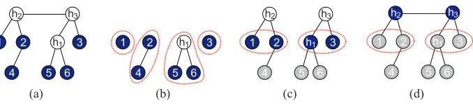
Figure 5: Illustration of CLRG. The shaded nodes are the observed nodes and the rest are hidden nodes. The dotted lines denote surrogate mappings for the hidden nodes so for example,

node 3 is the surrogate of h3. (a) The original latent tree, (b) The Chow-Liu tree (MST)

over the observed nodes V , (c) The closed neighborhood of node 5 is the input to RG, (d) Output after the first RG procedure, (e) The closed neighborhood of node 3 is the input to the second iteration of RG, (f) Output after the second RG procedure, which is same as the original latent tree.

2. Identify the set of internal nodes in MST(V ; D).

3. For each internal node i, let nbd[i; T] be its closed neighborhood in T and let S =

RG(nbd[i; T],D)be the output of RG with nbd[i; T]as the set of input nodes.

4. Replace the subtree over node set nbd[i; T]in T with S. Denote the new tree as T .

5. Repeat steps 3 and 4 until all internal nodes have been operated on.

Note that the only difference between the algorithm we just described and CLNJ is Step 3 in which the subroutine NJ replaces RG. Also, observe in Step 3 that RG is only applied to a small subset of nodes which have been identified in Step 1 as possible neighbors in the true latent tree. This reduces the computational complexity of CLRG compared to RG, as seen in the following theorem whose

proof is provided in Appendix A.5. Let_|J_|:=_|V_\Leaf(MST(V ; D))_|<m be the number of internal

nodes in the MST.

Theorem 10 (Correctness and Computational Complexity of CLRG) If the distribution Tp∈

T

Thus, the computational complexity of CLRG is low when the latent tree Tphas a small

maxi-mum degree and a small effective depth (such as the HMM) because (19) implies that∆(MST(V ; D))

is also small. Indeed, we demonstrate in Section 7 that there is a significant speedup compared to applying RG over the entire observed node set V .

We now illustrate CLRG using the example shown in Figure 5. The original minimal latent tree

Tp= (W,E)is shown in Figure 5(a) with W={1,2, . . . ,6,h1,h2,h3}. The set of observed nodes is

V=_{1, . . . ,6_}and the set of hidden nodes is H=_{h1,h2,h3}. The Chow-Liu tree TCL=MST(V ; D)

formed using the information distance matrix D is shown in Figure 5(b). Since nodes 3 and 5 are the

only internal nodes in MST(V ; D), two RG operations will be executed on the closed neighborhoods

Latent variables Distribution MST(V ; D) =TCL? Structure Parameter

Non-latent Gaussian X X X

Non-latent Symmetric Discrete X X X

Non-latent General Discrete _× X _×

Latent Gaussian X X X

Latent Symmetric Discrete X X X

Latent General Discrete _× X _×

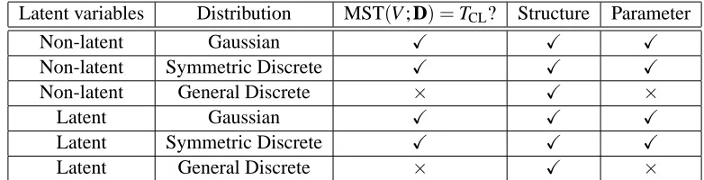
Table 1: Comparison between various classes of distributions. In the last two columns, we state whether CLGrouping is consistent for learning either the structure or parameters of the model, namely whether CLGrouping is structurally consistent or risk consistent respec-tively (cf., Definition 2). Note that the first two cases reduce exactly to the algorithm proposed by Chow and Liu (1968) in which the edge weights are the mutual information quantities.

RG. This is shown in Figure 5(c) where nbd[5; MST(V ; D)] =_{1,3,4,5_}, which is then replaced by

the output of RG to obtain the tree shown in Figure 5(d). In the next iteration, RG is applied to the

closed neighborhood of node 3 in the current tree nbd[3; T] =_{2,3,6,h1_}as shown in Figure 5(e).

Note that nbd[3; T]includes h1∈H, which was introduced by RG in the previous iteration. The

distance from h1 to other nodes in nbd[3; T]can be computed using the distance between h1 and

its surrogate node 5, which is part of the output of RG, for example, d2h1 =d25−d5h1. The closed

neighborhood nbd[3; T]is then replaced by the output of the second RG operation and the original

latent tree Tpis obtained as shown in Figure 5(f).

Observe that the trees obtained at each iteration of CLRG can be related to the original latent tree in terms of edge-contraction operations (Robinson and Foulds, 1981), which were defined in

Section 5.2. For example, the Chow-Liu tree in Figure 5(b) is obtained from the latent tree Tp

in Figure 5(a) by sequentially contracting all edges connecting an observed node to its inverse surrogate set (cf., Lemma 8(ii)). Upon performing an iteration of RG, these contraction operations are inverted and new hidden nodes are introduced. For example, in Figure 5(d), the hidden nodes

h1,h2 are introduced after performing RG on the closed neighborhood of node 5 on MST(V ; D).

These newly introduced hidden nodes in fact, turn out to be the inverse surrogate set of node 5, that

is, Sg−1(5) =_{5,h1,h2}. This is not merely a coincidence and we formally prove in Appendix A.5

that at each iteration, the set of hidden nodes introduced corresponds exactly to the inverse surrogate set of the internal node.

We conclude this section by emphasizing that CLGrouping (i.e., CLRG or CLNJ) has two primary advantages. Firstly, as demonstrated in Theorem 10, the structure of all minimal tree-structured graphical models can be recovered by CLGrouping in contrast to CLBlind. Secondly, it typically has much lower computational complexity compared to RG.

5.5 Extension to General Discrete Models

For general (i.e., not symmetric) discrete models, the mutual information I(Xi; Xj)is in general not

monotonic in the information distance di j, defined in (9).19 As a result, Lemma 6 does not hold,

that is, the Chow-Liu tree TCLis not necessarily the same as MST(V ; D). However, Lemma 8 does

hold for all minimal latent tree models. Therefore, for general (non-symmetric) discrete models, we

compute MST(V ; D)(instead of the Chow-Liu tree TCLwith edge weights I(Xi; Xj)), and apply RG

or NJ to each internal node and its neighbors. This algorithm guarantees that the structure learned

using CLGrouping is the same as Tp if the distance matrix D is available. These observations are

summarized clearly in Table 1. Note that in all cases, the latent structure is recovered consistently.

6. Sample-Based Algorithms for Learning Latent Tree Structures

In Sections 4 and 5, we designed algorithms for the exact reconstruction of latent trees assuming

that pV is a tree-decomposable distribution and the matrix of information distances D is available.

In most (if not all) machine learning problems, the pairwise distributions p(xi,xj) are unavailable.

Consequently, D is also unavailable so RG, NJ and CLGrouping as stated in Sections 4 and 5 are not directly applicable. In this section, we consider extending RG, NJ and CLGrouping to the case

when only samples x_Vn are available. We show how to modify the previously proposed algorithms

to accommodate ML estimated distances and we also provide sample complexity results for relaxed versions of RG and CLGrouping.

6.1 ML Estimation of Information Distances

The canonical method for deterministic parameter estimation is via maximum-likelihood (ML) (Ser-fling, 1980). We focus on Gaussian and symmetric discrete distributions in this section. The gener-alization to general discrete models is straightforward. For Gaussians graphical models, we use ML

to estimate the entries of the covariance matrix,20that is,

b

Σi j=

1

n

n

∑

k=1

x(_ik)x(_jk), _∀i,j∈V. (20)

The ML estimate of the correlation coefficient is defined asbρi j :=Σbi j/(bΣiiΣbj j)1/2. The estimated

information distance is then given by the analog of (8), that is, dbi j =−log|bρi j|. For symmetric

discrete distributions, we estimate the crossover probabilityθi j via ML as21

b

θi j=

1

n

n

∑

k=1

I_x(k)

i 6=x

(k)

j , ∀i,j∈V.

The estimated information distance is given by the analogue of (10), that is,dbi j=−(K−1)log(1−

Kbθi j). For both classes of models, it can easily be verified from the Central Limit Theorem and

continuity arguments (Serfling, 1980) thatdbi j−di j=Op(n−1/2), where n is the number of samples.

This means that the estimates of the information distances are consistent with rate of convergence

being n−1/2_{. The m×m matrix of estimated information distances is denoted asD}b_{= [d}b

i j].

6.2 Post-processing Using Edge Contractions

For all sample-based algorithms discussed in this section, we apply a common post-processing step using edge-contraction operations. Recall from (11) that l is the minimum bound on the information

20. Recall that we assume that the mean of the true random vector X is known and equals to the zero vector so we do not need to subtract the empirical mean in (20).