Semi-supervised learning and relevance search on networked data

(1)

c

(2)

SEMI-SUPERVISED LEARNING AND RELEVANCE SEARCH ON NETWORKED DATA

BY MING JI

DISSERTATION

Submitted in partial fulfillment of the requirements for the degree of Doctor of Philosophy in Computer Science

in the Graduate College of the

University of Illinois at Urbana-Champaign, 2013

Urbana, Illinois

Doctoral Committee:

Professor Jiawei Han, Chair & Director of Research Professor Dan Roth

Professor Thomas Huang

Associate Professor Yuguo Chen

(3)

Abstract

Real-world data entities are often connected by meaningful relationships, forming large-scale net-works. With the rapid growth of social networks and online relational data, it is widely recognized that networked data are playing increasingly important roles in people’s daily life. Based on whether the nodes and edges have different semantic meanings or not, networks can be roughly categorized into heterogeneous and homogeneous networks. Although homogeneous networks have been studied for decades, some problems still remain unsolved. Heterogeneous networks are much more complicated than homogeneous networks, and have not been explored until recently. There-fore, effective and principled algorithms for mining both homogeneous and heterogeneous networks are in great demand.

In this thesis, two important and closely related problems, semi-supervised learning and rele-vance search, are studied on both homogeneous and heterogeneous networks. Different from many existing models, algorithms developed in this thesis are theoretically reasonable, widely applicable with minimum constraints, and provide more informative mining results. First, a label selection criterion is proposed to improve the effectiveness of existing semi-supervised learning models on networks. Second, ranking and semi-supervised learning are integrated together to improve the in-formativeness of the results. Third, a relevance search algorithm that fully considers the geometric structure of the homogeneous networked data is designed. Finally, the relevance search problem between different types of nodes on heterogeneous networks is studied, and the proposed solution is applied on a network constructed from unstructured text data. Research results introduced in this thesis provide advanced principles and the first few steps towards a complete and systematic solution of mining networked data.

(4)

(5)

Acknowledgments

I would like to thank all the people and agencies who give me tremendous support and help during my PhD study in the past few years.

First and foremost, I would like to express my deepest gratitude and respect to my advisor, Prof. Jiawei Han, for his generous help, support and guidance throughout my PhD study. During my research, Prof. Han always provides insightful and visionary discussions, and encourages me to move forward. When I encounter difficulties in my life, he gives me wise suggestions and fully understands my situation. For me, Prof. Han is my advisor in both research and life. Without his support and understanding, I could not have overcome the most painful year in my life, nor would this thesis have been possible.

Moreover, I would like to thank other doctorate committee members, Prof. Dan Roth, Prof. Thomas Huang, Prof. Yuguo Chen and Prof. Jieping Ye, for their invaluable help during my research and constructive suggestions on this thesis.

I sincerely thank Prof. Xiaofei He and Prof. Deng Cai from Zhejiang University, Dr. Qi He from IBM Almaden Research Center, Prof. Rong Jin from Michigan State University, Dr. Jun Yan from Microsoft Research Asia, Marina Danilevsky, Yizhou Sun, Siyu Gu from Beijing Institute of Technology, Binbin Lin from Arizona State University and Tianbao Yang from GE Global Research for their constructive discussions and great support to my research. The outcome of the collaborations has made the very important pieces of this thesis.

I also owe sincere gratitude to my other collaborators including Bolin Ding, Jing Gao, Zhenhui Li, Cindy Xide Lin, Jialu Liu, Lu Su, Lu-An Tang, Chi Wang, Hongning Wang, Yintao Yu, W. Scott Spangler from IBM Almaden Research Center and Chiyuan Zhang from Massachusetts Institute of Technology. Thanks to all the professors and students in the Database and Information System (DAIS) group for their friendly support and stimulating discussions.

(6)

Finally and above all, I am indebted to my parents, Xinli Ding and Wei Ji, and my husband Nan Hua. Thank you for being together with me all the time and through all the difficulties. I love you.

(7)

List of Tables

3.1 Classification accuracy (%) by using 20 and 50 labels on the Isolet data set. . . 22

3.2 Classification accuracy (%) by using 20 and 50 labels on the MNIST data set. . . 23

3.3 Classification accuracy (%) by using 20 and 50 labels on the co-author graph. . . 24

4.1 Conferences from two research areas . . . 27

4.2 Top-5 ranked conferences in different settings . . . 27

4.3 Comparison of classification accuracy on authors (%) . . . 38

4.4 Comparison of classification accuracy on papers (%) . . . 38

4.5 Comparison of classification accuracy on conferences (%). . . 38

4.6 Top-5 conferences related to each research area generated by different algorithms . . 42

4.7 Top-5 terms related to each research area generated by different algorithms . . . 42

5.1 Performance evaluated by different metrics on the COREL data set. . . 61

5.2 Performance evaluated by different metrics on the CMU PIE data set . . . 61

5.3 Performance evaluated by different metrics on the Yale-B data set . . . 61

5.4 Performance evaluated by different metrics on the 20 Newsgroups data set . . . 65

5.5 Performance evaluated by different metrics on the TDT2 data set . . . 65

5.6 Performance evaluated by different metrics on the Reuters data set . . . 65

6.1 Compare different meta paths and their combination. . . 85

(10)

List of Figures

3.1 Classification accuracy vs. the number of labels used on the Isolet data set . . . 22

3.2 Classification accuracy vs. the number of labels used on the MNIST data set . . . . 23

3.3 Classification accuracy vs. the number of labels used on the co-author graph. . . 24

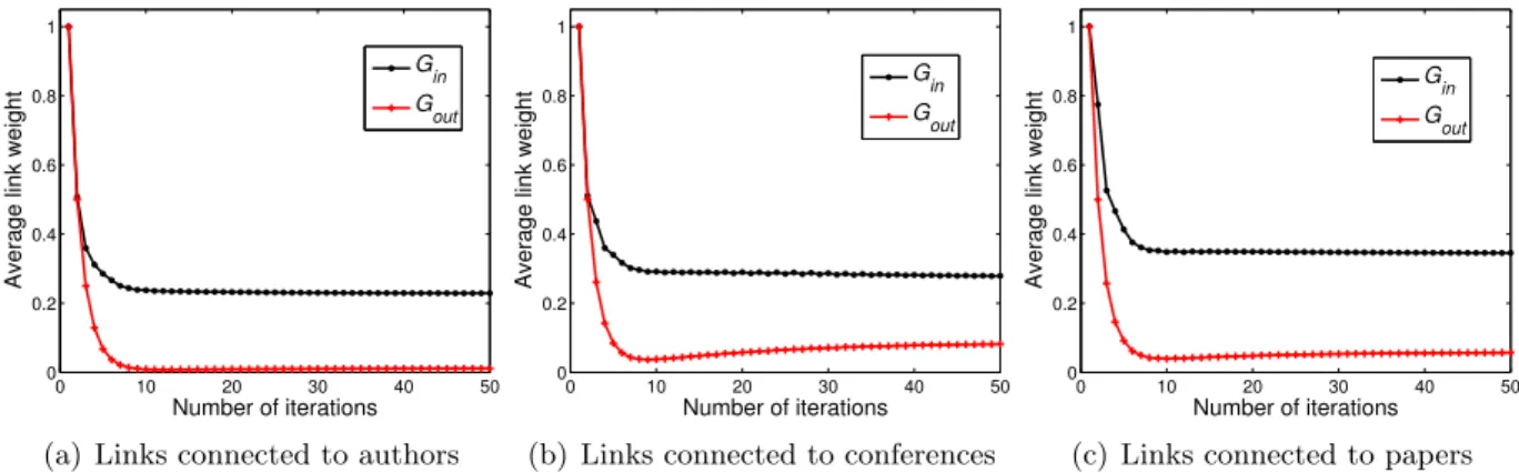
4.1 Link weight change in 50 iterations . . . 40

4.2 Model Selection when (0.5%, 0.5%) of authors and papers are labeled . . . 43

4.3 Running time w.r.t. database size. . . 43

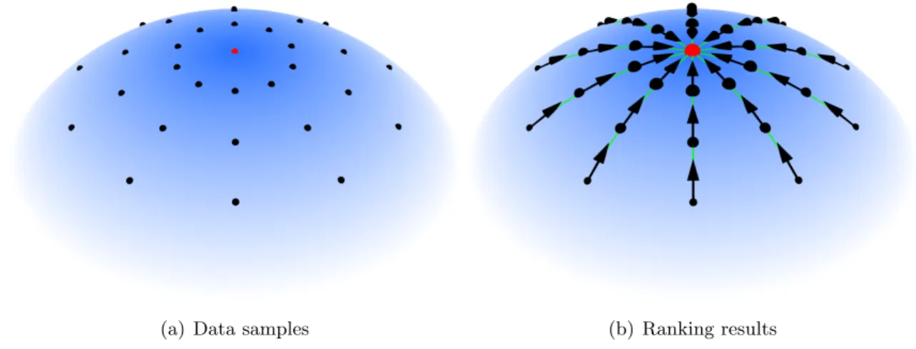
5.1 We aim to design a relevance function that has the highest value at the query point marked by red, and then decreases linearly along the geodesics of the manifold, which is equivalent to its gradient field being parallel along the geodesics. The arrows above denote the gradient field of the relevance function, and the green lines denote the geodesics of the data manifold. . . 45

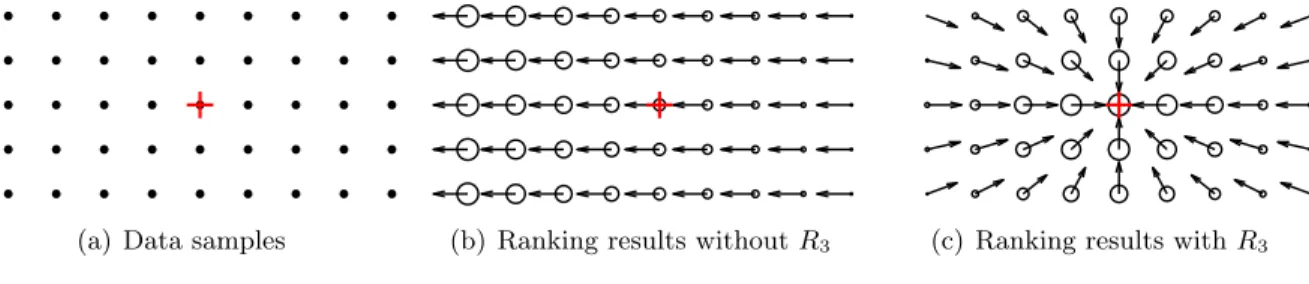
5.2 A toy example explaining the reason of addingR3. . . 50

5.3 Performance comparison of various relevance search algorithms on a toy data set. (a) shows the data set sampled from a Swiss roll with a hole, where the query is denote by ‘+’. (b) shows the ranking order generated by PFRank. We can see that PFRank successfully preserves the ranking order of the data points along the geodesics of the manifold. For example, the geodesic distance between the query and the point marked by ‘N’ is smaller than that between the query and the point marked by ‘’. So ‘N’ is ranked higher than ‘’. (c) shows the ranking order generated by MR. We can see that ‘N’ is ranked lower than ‘’, which is counterintuitive. (d) shows the ranking order generated by SVM, which does not take the manifold structure into consideration. (e) and (f) show the vector field and the gradient field of the relevance function learned by PFRank, respectively, which are quite parallel and point to the query. (g) and (h) show the gradient fields of the relevance functions learned by MR and SVM, respectively, which do not vary smoothly along the manifold. . . 57

5.4 The average precision-scope curves of different algorithms on three image data sets.. 61

5.5 Model selection on the COREL data set.. . . 62

5.6 Model selection on the CMU PIE data set. . . 62

5.7 Model selection on the Yale-B data set. . . 62

5.8 The average precision-scope curves of different algorithms on three document corpora. 64 5.9 Model selection on the 20 Newsgroups data set. . . 66

5.10 Model selection on the TDT2 data set. . . 66

5.11 Model selection on the Reuters data set. . . 66

(11)

6.2 System framework of EntityRel.. . . 71

6.3 Entity Correlation Graph G. One edge = 1,000 links in data. The size of circle is proportional to # of entities. . . 75

6.4 Degree distribution of the nodes in G. . . 76

6.5 Histogram of # of times that the ground truth drug-disease pairs co-occur in text corpusD. . . 82

6.6 Comparecorrelation toco-occurrence. . . 83

6.7 Compare different meta paths and their combination in Precision/Recall based on EntityRel. . . 85

(12)

Chapter 1

Introduction

Nowadays, data represented in the form of graphs and networks are playing increasingly important roles in real life. Examples include friendship networks in Facebook1, co-author networks extracted from bibliographic data, webpages interconnected by hyperlinks on the Web, etc. In these scenarios, data instances are connected by edges representing meaningful relationships. I use graphs and networks interchangeably to represent the same concept in this thesis. Networks and feature vectors are two alternatives to represent the data, and the former is often more natural than the latter in many important applications [24]. Even if the data is traditionally represented in a feature space, it is usually helpful to transform the data into a network, or graph structure (for example, by constructing a nearest neighbor graph) to better exploit the intrinsic characteristics of the data. Therefore, mining networked data is of a great interest to both industry companies and academia. Most of the existing studies about networks mainly work with homogeneous networks, i.e., net-works composed of a single type of nodes, as mentioned above. However, heterogeneous netnet-works composed of multiple types of nodes are more general and prevalent in many real world applica-tions. For example, beyond co-author networks, bibliographic data actually forms a heterogeneous network consisting of multi-typed nodes, such as papers, authors, venues and terms. Other exam-ples include biomedical networks among drugs, diseases, targets and MeSH terms, and E-commerce networks composed of sellers, customers, items and tags.

My past and current research focuses on mining both homogeneous and heterogeneous networks, with a main concentration on semi-supervised learning and relevance search of the nodes. Semi-supervised learning is a classical topic aiming at inferring the labels on all the data given some label information on part of the data, while both labeled and unlabeled data are utilized throughout the learning process. When applied to the graph data, it has wide applications including research

1

(13)

community discovery, fraud detection, product recommendation, etc. Semi-supervised learning often performs better than unsupervised learning by employing the valuable human labels, and often needs much fewer labels than supervised learning, therefore attracting substantial attention in the past few years. Although semi-supervised learning has been extensively studied in literature, how to further improve the performance of an existing semi-supervised learning algorithm on networked data is still underexplored. During my PhD study, I have developed a variety of techniques to tackle this problem, generating robust and meaningful prediction results on networks with a very small portion of labeled data. Given an existing semi-supervised learning framework on networked data, there are generally two directions to further improve its performance: (1) minimize its expected error by providing it with the best data configuration, such as an informative subset of data to label, which falls into the topic of active learning [36][31], or a good feature representation of the data, which can be cast as a feature selection problem [32]; and (2) make the results more informative by providing a good summary and understanding of the results [37]. I will discuss my progress in both directions in this thesis.

Relevance search is another important function on networked data. Given a query node in a network, we aim to learn a real-valued relevance function f such that for any two nodes vi and

vj, f(vi) > f(vj) if vi is more relevant to the query than vj, and vice-versa. Note that the final

goal of relevance search is to rank all the nodes according to their relevance to the query node, where the top ranked nodes are closely relevant to the query and therefore are presented to the user. Therefore, relevance search is one kind of ranking problem. In this thesis, we use “relevance search” and “ranking” to denote two different problems, where the former one computes arelevance

score for each node with regarding to the query node, and the latter one computes aranking score for each node without specifying the query node. Relevance search and semi-supervised learning are actually closely related in literature if we use “relevant” as the meaning of the labels. For example, semi-supervised learning frameworks have been adapted to solve the relevance search problem [90] by treating the query node as the only labeled node. In this thesis, I will introduce a novel relevance search framework on homogeneous networked data, which follows the idea of a recently proposed semi-supervised learning model [47] and fully considers the special requirement of the relevance search problem. A more challenging problem is how to perform relevance search

(14)

over heterogeneous networks. This is also addressed in this thesis over a heterogeneous network constructed in the biomedical domain.

The points below highlight the contributions of this thesis:

• I study how to selectively choose nodes to label such that the expected error of a state-of-the-art semi-supervised learning framework on homogeneous networked data can be minimized [36]. A novel variance minimization criterion is proposed to solve this problem. Compared to existing label selection criterion, our algorithm has the advantage of selecting nodes to label in a batch offline mode with solid theoretical support. By employing our proposed approach, the quality of the labels, as well as the performance of the semi-supervised learner on homogeneous networks, is theoretically improved.

• I explore the problem of integrating ranking and semi-supervised classification to improve the semi-supervised classification performance in heterogeneous networks [37]. By letting ranking and semi-supervised classification iteratively enhance each other, the classification results of the nodes are not only more accurate, but are also more informative since the ranking of nodes within each class provide a good understanding and summary of each class.

• I try to propose a better relevance search algorithm on homogeneous networked data under the assumption that each node in the network has a high-dimensional feature representation, and the nodes are sampled from a submanifold embedded in the ambient Euclidean space [38]. Ideally, beyond smoothness, a desirable relevance function should vary monotonically along the geodesics of the manifold. Therefore, the order of the nodes along the geodesics of the manifold could be well preserved. Moreover, according to the nature of the relevance search problem, no sample in the data set should be more relevant to the query than the query itself. So the relevance function should have the highest value at the query node, and then decrease to other nodes nearby. Our proposed algorithm effectively learns a relevance function that has the highest value at the query node, and varies linearly and therefore monotonically along the geodesics of the data manifold. • I study the problem of discovering strong relevance between heterogeneous typed biomedical

entities using a network-based model. Considering the fact that we do not have a heteroge-neous network among biomedical entities available for study, we first construct a heterogeheteroge-neous

(15)

biomedical network from massive biomedical text data. Following the meta path philosophy [74], we select the top-k meta paths that are the most useful for our relevance search task. Equipped with meta path constrained relationship contexts, we design a model to compute the strong relevance between two heterogeneous entities, named EntityRel. Our intuition is, two entities of heterogeneous types are strongly relevant if they are connected by many paths with high weight following the selected meta paths.

The rest of this thesis is organized as follows. Chapter 2 provides an overview of the related work. Chapter 3 ∼ 6 present my work in semi-supervised learning and relevance search over networked data. Finally, I conclude this thesis in Chapter 7.

(16)

Chapter 2

Related Work

As my thesis focuses on improving semi-supervised learning and relevance search on networked data, it is related to the study ofactive learning,semi-supervised classification,ranking, Laplacian-based relevance search on homogeneous data, andrelevance search on heterogeneous data. A brief overview of these related methods is discussed in this chapter.

2.1 Active Learning

Most of the existing active learners work with data represented by feature vectors [68]. A seminal paper [31] proposes the first manifold-based active learning algorithm, i.e., GRED, which takes into account both the discriminant and geometrical structure in the data. A nearest neighbor graph is constructed to model the intrinsic manifold structure and incorporated into a least squares loss function as a regularizer. The most informative data points are selected by minimizing the size of the parameter covariance matrix. This principle has been successfully applied to image retrieval [30], video indexing [86], and feature selection [32]. Please see [8] for another active learning approach that exploits the features together with the graph structure. However, in some cases, features of the graph nodes are not always available. Some other methods try to select data based on the graph structure and some labeled nodes. Existing approaches have considered selecting the data that the current classifier is the most uncertain [52], the data with maximum expected information gain [88] or maximum expected entropy reduction [50]. Based on the Gaussian random field model [92], an empirical risk minimization framework [93] is proposed to select examples that minimize the empirical risk estimated by the current classifier. One major limitation of these methods [93,52,33,88,50,41] is that they have to obtain the labels of the selected nodes in order to select more data, therefore are not applicable when there is no label information provided during

(17)

active learning. When labeling an instance requires time consuming and expensive experiments, these methods are much more costly than running a batch offline mode active learner once and perform labeling in parallel [24].

Recently, there are some efforts devoted to designing label selection criteria that use the graph structure only, without feature representation and label information. Intuitively, one tends to select nodes that lie in high-density (unlabeled) regions [41] or the centers of clusters [52], or have high impact (measured by the graph structure) to unlabeled data [71]. However, these intuitive selection criteria do not have theoretical support on optimizing any classifier.

It is worth mentioning that designing active learners on graphs aiming at minimizing the error of a particular classifier has received substantial interest recently [24,93]. [24] provides theoretical bounds of the prediction error which are related to label smoothness over the graph, justifying the reasonableness of clustering the nodes and then randomly choose one point from each cluster. Compared with existing methods [24,93,8,41], our proposed algorithm [36] has the advantage of directly minimizing the expected error (instead of the upper bound of the error) in a batch offline mode, through reasonably modeling the probability distribution over the graph. Therefore, we do not require the (potentially expensive) label information of the selected data and tedious retraining of the classifier repeatedly.

2.2 Semi-supervised Classification

Semi-supervised classification is an essential tool in analyzing networked data when the label infor-mation is available for some nodes [87,73]. Collective classification [51,66,56] has been proposed to employ both the network structure and the feature representation of nodes in the classification task. Since local features may not be always available, Macskassy et al. [53] develop a relational neighbor classifier to classify network-only data by iteratively assigning a node to the majority class of its neighbors. This idea is similar to the label propagation scheme in graph-based classification [89], where each point iteratively spreads its label information to neighbors so as to ensure both local and global consistency. Based on the same label smoothness assumption, Zhu et al. [92] for-mulate the problem using a Gaussian random field model defined with respect to the graph. And the framework of manifold regularization [6] is proposed for data-dependent regularization that

(18)

exploits the geometry of the probability distribution on the labeled and unlabeled data. However, existing algorithms mainly work on homogeneous networks and graphs, and therefore cannot easily distinguish between the type differences among nodes in a heterogeneous network. Recently, the graph-based classification framework has been extended to work on heterogeneous networked data [39]. In this thesis, we enhance the label propagation framework by providing within-class rank-ing for nodes in the network, which can improve classification results by providrank-ing an informative summary of each class [37].

To enhance the quality of classification, boosting, bagging and ensemble methods have been explored in various studies [28]. In particular, boosting methods such as AdaBoost [18] iteratively learn from their classification mistakes by assigning higher weights to nodes which are misclassified in each previous round, until a stable classification state is reached. Like boosting, our proposed method [37] also adjusts the relative importance of nodes in various rounds of classification. How-ever, [37] uses within-class ranking to measure the importance of each node with regard to each class, in contrast to boosting, which estimates the global importance of each node based on classi-fication mistakes.

2.3 Ranking

As data sets with inherent network structures become increasingly prevalent, ranking networked data has received substantial interest in recent years. Two important representative algorithms are PageRank [60] and HITS [40], both of which propagate information throughout the network to compute the ranking score of each node, using different propagation methods corresponding to different ranking rules. These methods mainly work on homogeneous networks. Recently, PopRank [58] was proposed to rank the popularity of heterogeneous web objects via knowledge propagation throughout the heterogeneous network of web objects. This approach considers that different types of links in a network have different propagation factors, which are trained according to partial ranks given by experts. In contrast, we rank nodes according to their importance within each class, rather than within the global set of all the nodes, and the ranking results in turn facilitate more accurate classification.

(19)

methodology to cluster nodes in heterogeneous networks, which is closely related to my study. Although this method effectively provides a ranking within each cluster, it has some limitations: (1) it can only work on heterogeneous networks with a star schema; and (2) it requires a prior distribution specified by several labeledrepresentative nodes of each cluster, and does not work well with arbitrary labeled nodes, which may not be representative. Thus, if we do not know which nodes are representative in a data set, NetClus cannot be used. However, for heterogeneous networks with arbitrary network schema, our proposed algorithm [37] can make full use of label information available for any nodes to generate accurate classification results and informative rankings.

2.4 Laplacian-based Relevance Search

For relevance search methods under the manifold assumption, the most related work is the Laplacian-based relevance search method [90]. Here we give a brief introduction of [90].

Let M be a d-dimensional submanifold in the Euclidean space Rm. Given n data points

{x1, . . . , xn} ∈Rm on M, wherexq is the query (1≤q≤n), we aim to learn a relevance function

f :M →_R, such that ∀i, j∈ {1, . . . , n}, f(xi)> f(xj) if xi is more relevant to the queryxq than

xj, and vice-versa.

The intuition behind [90] is that if two pointsxi andxj are linked together in a graph/network,

then their relevance scoresf(xi) andf(xj) should be close as well. LetW ∈Rn×nbe a symmetric

affinity matrix of the network, and y = [y1, . . . , yn]T be an initial relevance score vector which

encodes some prior knowledge about the relevance of each data point to the query. Then [90] minimizes the following objective function:

JM R(f) = n X i,j=1 wij( f(xi) √ Dii −_pf(xj) Djj )2+µ n X i=1 (f(xi)−yi)2 (2.1)

where wij denotes the element at the i-th row and j-th column of W, µ > 0 is a regularization

parameter and D is a diagonal matrix used for normalization with Dii = Pn_j=1wij. The first

term in the above function aims to learn a relevance function that varies smoothly along the data manifold. The second term ensures the finally estimated relevance scores to be close to the initial relevance score assignment y.

(20)

Let f = [f(x1), . . . , f(xn)]T. The closed form solution of Eq. (2.1) is the following:

f∗ = (µI+L)−1y (2.2)

where I is an identity matrix of size n×n. L = I −D−1/2W D−1/2 is the normalized Graph Laplacian [14]. We can also obtain the same solution via an iterative scheme:

ft+1 = 1

µ+ 1Sf

t₊ µ

µ+ 1y (2.3)

where each data point spreads the relevance score to its neighbors iteratively.

The above relevance search framework based on Laplacian regularization has enjoyed long-lasting popularity in the community, with successful extensions in content-based image retrieval [29], relevance search on both undirected and directed graphs [1], ranking on multi-typed inter-related web objects [22], ranking tags over a tag similarity graph [48], etc. However, for the Laplacian-based relevance search framework, we do not exactly know how the relevance function varies, and whether the order of the data points is preserved along the geodesics of the data man-ifold. [91] points out some drawbacks of [90] and proposes a more robust method by using an iterated graph Laplacian. But [91] still works under the Laplacian-based relevance search frame-work, addressing the smoothness of the function. Besides, the Laplacian-based relevance search framework requires the final relevance estimation results to be close to the initial relevance score assignmenty. In the situation when there is no prior knowledge about the relevance of each data point, people usually assign yi= 1 if xi is the query andyi= 0 otherwise. This might not be very

reasonable, and the finally estimated relevance scores are likely to be biased towards the initial relevance score assignment.

2.5 Relevance Search On Heterogeneous Data

As pointed out in [69] [3], the relationships between entities are the heart of the Semantic Web. Substantial efforts are made to develop techniques for searching complex relationships between entities [3][2] [4]. The relationships are often referred to as Semantic Associations. However, those

(21)

Semantic Associations studied in Semantic Web are mainly based on the RDF model, therefore are restricted to simple, existing relationships, such as the “purchase” relationship between customers and items, the “work for” relationship between professors and universities, etc. Different from those existing work, we focus on discovering meaningful relevance relationships that do not explicitly exist in any structured data.

Another family of related work is the recommendation systems, which suggest the items that the users are likely to be interested in [67] [83] [23]. Although recommendation also discovers relevance relationships between two different types of entities (users and items), our problem is fundamentally different from the classical recommendation problem. Specifically, we aim to develop a fully automatic approach that does not use any label information, while recommendation systems usually know some users are interested in certain items.

Given a graph, many methods have been developed for estimating relevance between two nodes, with the Laplacian-based relevance search framework described above being a representative on the homogeneous graphs. For heterogeneous graphs, PathSim [74] gives an interesting meta path based similarity measure between two nodes of the same type. HeteSim [70] and Path Constrained Random Walk [46] estimate the relevance between different types of nodes following the random walk framework. However, the original HeteSim algorithm only uses the binary graph, ignoring the weight on the edges, which is shown to be critically important in our experiments. Path Constrained Random Walk favors the popular entities undesirably and ignores the differences of various contexts inherited from various meta paths. More discussion about these methods can be found in Section6.5.1

(22)

Chapter 3

Label Selection in Semi-supervised

Learning on Homogeneous Graphs: A

Variance Minimization Criterion

3.1 Overview

Substantial efforts have been devoted to the problem of semi-supervised learning on the nodes in a homogeneous graph. On the other hand, labels can be very expensive to obtain in many real-world applications. Label selection, or active learning methods [15] are then proposed to determine which data examples should be labeled such that the learner could achieve higher prediction accuracy over the unlabeled data as compared to random label selection. Here we use label selection and active learning to denote the same problem. The goal of active learning is to maximize the learner’s ability given a fixed budget of labeling effort. While many effective active learners have been developed in literature [68], active learning that takes direct advantage of the graph structure in the data has not been explored until recently [24,8,93]. As large-scale data sets with inherent graph structures become increasingly prevalent, reasonable and natural active learning criteria on graphs are in great demand.

In this work, we propose a novel variance minimization perspective to active learning purely on the graph structure, without feature representation and label information. Our study is based on the common assumption that the labels vary smoothly with respect to the graph, which is widely used in the graph-based semi-supervised learning literature [13,9,26,61,7]. Following one of the most popular graph-based learning frameworks [92], we formulate the smoothness assumption by a Gaussian random field over the graph nodes. Theoretical analysis indicates that the Gaussian field over the unlabeled vertices, conditioned on the labeled data, is a multivariate normal whose mean is the prediction of the harmonic Gaussian field classifier [92]. It is interesting to note that the covariance matrix of the Gaussian field over the unlabeled data is not dependent on the class labels, but only on the graph structure. In this way, we propose to select the data points to label

(23)

such that the total variance of the Gaussian field over unlabeled examples, as well as the expected prediction error of the harmonic Gaussian field classifier, is minimized. Efficient computation scheme is then proposed to solve the corresponding optimization problem without introducing any additional parameter.

3.2 Minimizing the Expected Error of Semi-supervised Learning

on Graphs

3.2.1 The Problem

We define the active learning problem on graphs as follows. Given a graph G =hV,Ei associated with a weight matrixW, whereV ={v1, . . . , vn}is the set of data points (without feature

represen-tation) with true labels y= (y1, . . . , yn)T, E is the set of edges between any two data points in V,

and W = (wij)∈Rn×n where wij denotes the weight on the edge between two data pointsvi and

vj. Our goal is to find a subset of pointsL={vp1, . . . , vpl} ⊂ V where{pi}

l

i=1⊂ {1, . . . , n}are the

indices of the points that we should label, such that the classifier learned from the labels onLcould achieve the smallest expected prediction error on the unlabeled data, measured byP

vi∈U(yi−y ∗ i)2,

whereU =V \ L andy_i∗ is the predicted label forvi.

Without loss of generality, here we assume thatGis undirected and connected. We allow contin-uous labels here, and the labels are assumed to vary smoothly over the graph, i.e.,P

i,jwij(yi−yj)2

is small, which is similar to [24].

3.2.2 The Objective Function

Following [92, 93], the label smoothness assumption could be formulated by a Gaussian random field over the graph:

P(y) = 1

Zβ

exp(−βE(y)) (3.1)

where E(y) = 1₂P

i,jwij(yi−yj)2 is the energy function measuring the smoothness of a label

assignment y= (y1, . . . , yn)T over the graph, β is an “inverse temperature” parameter, andZβ is

a partition function for the normalization purpose.

(24)

l instances, i.e., L = {v1, . . . , vl}, and the rest u(= n−l) examples U = {vl+1, . . . , vl+u} are

unlabeled. Based on the Gaussian random field model, and the constraint that the predictions on the labeled set are consistent with ground truth, i.e., y∗_L=yL= (y1, . . . , yl)T, a standard method

is to predict the labels with the highest probability (or equivalently, minimum energy) [92,93]. Let

L=D−W be the graph Laplacian [14], where D is a diagonal matrix andDii=P_jwij. L can

be split into 4 blocks according to thel-th row and column:

L=    Lll Llu Lul Luu    (3.2)

Then the prediction on the unlabeled nodes given by the harmonic Gaussian field classifier is [92]:

y∗_U =−L−_uu1LulyL (3.3)

wherey_U∗ = (y_l+1∗ , . . . , y∗_l+u)T.

It can be proven that the Gaussian field, conditioned on the labeled data, is a multivariate normal: yU ∼ N(y∗U, L−uu1) [93], where yU = (yl+1, . . . , yl+u)T. Then we compute the expected

prediction error on the unlabeled nodes as follows:

E   X vi∈U (yi−y∗i)2   = E (yU −y∗U)T(yU −y∗U) = E Tr (yU −y∗U)(yU −yU∗)T = Tr E (yU −y∗U)(yU −yU∗)T = Tr (var(yU)) = Tr(L−uu1) (3.4)

In order to minimize the expected error of the prediction results, we should minimize the variance of the statistical learning model [15]. Therefore, we propose to select the nodes to label by solving the following optimization problem:

arg min

L⊂V

(25)

It is easy to verify that Eq. (3.5) is independent of the order of the examples, but only dependent on the choice of the set of the nodes that we choosenot to label. Therefore, our objective function is well defined.

3.3 Efficient Optimization

Let{q1, . . . , qu}be the indices of the nodes that we choosenot to label. Following the above

discus-sion, our objective is to select au×usubmatrixLuuofLon the intersections of the{q1, . . . , qu}-th

rows and columns, such that the trace of L−_uu1 is minimized. This optimization problem in Eq. (3.5) is challenging since the number of candidate sets for L is exponential in the total number of examples n. Moreover, since the number of unlabeled examples is usually huge,Luu will likely

be a large matrix and directly optimizing Eq. (3.5) based on the set of unlabeled data is very computationally expensive. In this section, we first transform the objective function so that it can be represented by the instances that we choose to label, and then propose an efficient sequential optimization scheme.

3.3.1 Formulations

We first construct a selection matrixS ∈_Ru×n _{to help selecting} _L

uu from Las follows: Sij =      1 ifj=qi 0 otherwise. Then we have: Luu=SLST (3.6)

Since Lis symmetric, it has the eigendecomposition result as follows:

(26)

such thatXis an orthonormal matrix, and Σ = diag{λ1, . . . , λn}, where{λi}ni=1are the eigenvalues

of L, and λ1 ≥. . .≥λn= 0. Then

Luu=SLST =SXΣXTST (3.8)

Suppose X = (x1, . . . ,xn)T, where xT_i is the i-th row of X. Let Q = SX, then Luu = QΣQT.

SinceS is the selection matrix, then Q= (q₁, . . . ,q_u)T ∈_Ru×n_{consists of the}_{_q

1, . . . , qu}-th rows

ofX. We further define two sets of vectorsX ={x1, . . . ,xn},Q={q1, . . . ,qu}, then our objective

function in Eq. (3.5) is equivalent to the following:

arg min

Q⊂X

Tr (QΣQT)−1

(3.9)

LetIn denote the identity matrix of size n×n. By using the Woodbury formula [21], we have the

following: (QΣQT)−1 = Q(Σ +In)QT −QQT −1 = Q(Σ +In)QT −Iu −1 = (−Iu)−1−Q (Σ +In)−1+QT(−Iu)−1Q −1 QT = −Iu−Q M−1−QTQ −1 QT

(27)

whereM = Σ +In= diag{λ1+ 1, . . . , λn+ 1}. According to the matrix determinant lemma [27], we have: det M−1−QTQ = (−1)ndet −M−1+QTQ = (−1)ndet −M−1 detIu+Q −M−1 −1 QT = (−1)2ndet M−1det Iu−QM QT = det Iu−QΣQT −QInQT n Y i=1 1 λi+ 1 = det (Iu−Luu−Iu) n Y i=1 1 λi+ 1 = det(−Luu) n Y i=1 1 λi+ 1 (3.10)

As long as 0 < u < n and the graph is connected, it can be easily proven that Luu is invertible,

and so isM−1−QTQ. Recall that Tr(AB) = Tr(BA), we further have:

Tr (QΣQT)−1 = −u−Tr Q M−1−QTQ−1QT = −u−Tr M−1−QTQ−1QTQ = −u+ Tr M−1−QTQ−1 (−QTQ+M−1−M−1) = −u+ Tr In− M−1−QTQ −1 M−1 = n−u−Tr M−1−QTQ−1 M−1 = l−Tr   M −1₋ u X i=1 q_iqT_i !−1 M−1  

(28)

Let P = {p₁, . . . ,p_l} = X \ Q be the {p1, . . . , pl}-th row vectors of X that correspond to the

examples that we choose tolabel, then we have:

Tr (QΣQT)−1 = l−Tr   M −1₋ u X i=1 q_iqT_i !−1 M−1   = l−Tr   M −1₋ n X i=1 xixTi + l X i=1 p_ipT_i !−1 M−1   = l−Tr   M −1₋_XT_X₊ l X i=1 p_ipT_i !−1 M−1   = l−Tr   M −1₋_I n+ l X i=1 p_ipT_i !−1 M−1  

Let A0 = M−1 −In. Since the number of data points to be labeled, l, is fixed, our objective

function in Eq. (3.9) reduces to the following:

arg max P⊂X Tr   A₀+ l X i=1 p_ipT_i !−1 M−1   (3.11)

In the following, we describe an efficient sequential optimization scheme to select which nodes we should label in a graph.

3.3.2 Selecting the First Point

Setting l = 1 in Eq. (3.11), we obtain the objective function of selecting one (or the first) data point to label: arg max p∈X Tr A0+ppT −1 M−1 (3.12)

(29)

Usually, matrix inversion formulae in the form of A0+ppT

−1

can be simplified using the Sherman-Morrison formula [21]:

(A+uvT)−1=A−1−A

−1_uvT_A−1

1 +vT_A−1_u (3.13)

However, note that

A0 = M−1−In = diag 1 λ1+ 1 −1, . . . , 1 λn+ 1 −1 = diag −λ1 λ1+ 1 , . . . , −λn λn+ 1 (3.14)

is singular since the smallest eigenvalue ofL(denoted asλn) is equal to 0. Therefore, the

Sherman-Morrison formula (3.13) cannot be applied here. In this subsection, we derive how to select the first point to label by performing some modification of Eq. (3.12).

For a connected graph, it is known that all the eigenvalues of L, except λn, are larger than 0.

The eigenvector corresponding toλn is an×1 constant vector which can be denoted as (c, . . . , c)T.

So anyp∈ X can be represented asp= (vT, c)T wherevis a (n−1)×1 vector after removing the last element of p. LetB = diagn−λ1

λ1+1, . . . ,

−λn−1

λn−1+1

o

∈R(n−1)×(n−1) be the matrix after removing

the last row and column ofA0, which is invertible. Hence:

A0+ppT =    B cv cvT c2   +    v 0    vT 0 = Bˆ+ ˆvvˆT where ˆB =    B cv cvT c2   and ˆv= ( v

T _{0 )}T_{. By doing blockwise matrix inversion, we have:}

ˆ B−1 =    B−1 0 0 0   + 1 c2₍₁₋_vT_B−1_v₎    c2B−1vvTB−1 −cB−1v −cvT_B−1 ₁   

(30)

whereB−1 _{= diag}n₋λ1+1

λ1 , . . . ,−

λn−1+1

λn−1

o

. Now we can employ Eq. (3.13) and have:

A0+ppT −1 = Bˆ+ ˆvvˆT−1 = Bˆ−1−Bˆ −1_v_ˆ_v_ˆT_B_ˆ−1 1 + ˆvTBˆ−1_v_ˆ (3.15)

Recall that M−1 _{= diag}n 1 λ1+1, . . . , 1 λn+1 o . Therefore, A0+ppT −1 M−1 _{can be computed}

efficiently without matrix inversion for any given p. We select the first data point to label that corresponds to p∈ X such that Eq. (3.12) is maximized.

3.3.3 Selecting More Points

We define: Al=A0+ l X i=1 p_ipT_i (3.16)

Supposel(≥1) data points have been selected, which correspond to the rows ofX: {p₁, . . . ,p_l}= P_l ⊂ X, then the (l+ 1)-th instance can be selected by solving the following:

p_l+1= arg max

p∈X \Pl

Tr Al+ppT

−1

M−1 (3.17)

By using the Sherman-Morrison formula (3.13), we have:

Al+ppT −1 =A−_l 1−A −1 l ppTA −1 l 1 +pT_A−1 l p (3.18)

And A−₁1 can be computed using Eq. (3.15). Therefore:

Tr Al+ppT −1 M−1 = Tr(A−_l 1M−1)−Tr A −1 l ppTA −1 l M −1 1 +pT_A−1 l p = Tr(A−_l 1M−1)−Tr p T_A−1 l M −1_A−1 l p 1 +pT_A−1 l p = Tr(A−_l 1M−1)−p T_A−1 l M −1_A−1 l p 1 +pT_A−1 l p (3.19)

(31)

Since Tr(A−_l 1M−1) is a constant when selecting the (l+ 1)-th data point, we choose the (l+ 1)-th point to label that corresponds to the following p_l+1:

p_l+1= arg min p∈X \Pl pTA−_l1M−1A−_l 1p 1 +pT_A−1 l p (3.20)

Once p_l+1 is obtained,Al+1 can be updated according to Eq. (3.18).

3.4 Experimental Results

In this section, we apply our proposed active learning method based on Variance Minimization (denoted asVM) in the Gaussian random field to several real-world data sets to test its effective-ness. We use the labels of vertices chosen by different active learning criteria to train a harmonic Gaussian field classifier [92] to predict the labels of the rest of the nodes in the graph. The following five label selection methods are compared:

• Our proposed VM algorithm (VM). • Empirical Risk Minimization (ERM) [10]. • Random selection (Random).

• Label Selection based on Clustering (LSC) [24]. • Uncertainty sampling (Uncertainty).

When our budget is to selectlinstances to label, theLSCmethod clusters the data into lclusters and then randomly select one example from each cluster. This method minimizes the prediction error bound related to label smoothness, and empirically performs the best in [24]. We use Spectral Clustering [57] to cluster the graph nodes. The results of Random and LSC are both averaged over 10 random trials. ERMand Uncertaintyare two methods that iteratively query more data to label according to the classifier trained by the previously labeled data. ERM selects examples that minimize the empirical risk estimated by the current classifier. The Uncertainty criterion selects the instances whose labels the current classifier is the most uncertain. Recall that the harmonic Gaussian field classifier adopts the one-against-all scheme in multi-class classification.

(32)

Suppose we have k classes and u unlabeled data points, then the classifier outputs a u×k score matrix, where each row is for an unlabeled point, and each column for a class. The class with the largest value in thei-th row is the predicted class of thei-th unlabeled point. Letf1(vi) denote the

largest score of nodevi related to a certain classk1, andf2(vi) denote the second largest score ofvi

related to a different classk2. The smallerf1(vi)−f2(vi), the more uncertain the classifier is about

the label prediction ofvi. Therefore, we select new instances {vi}to label with the smallest values

off1(vi)−f2(vi). This strategy is also compared in [52]. Notice thatERMand Uncertaintyuse

the label information of the previously selected data, while other active learning methods do not. In order to test them in our scenario that very little (if not none) label information is available during active learning, forERMandUncertainty, we randomly choose an initial set of labels for each of them, rank the other nodes according to the score of their label selection criterion (empirical risk forERM,f1(vi)−f2(vi) forUncertainty), and select the top ranked nodes. The performance of ERM and Uncertaintyare also averaged over 10 random selections of the initial set of labels.

In the following, we begin with a description of the data preparation.

3.4.1 Data Preparation

Three real-world data sets are used in our experiments. The first one is the Isolet spoken letter database 1. It contains 150 subjects who spoke the name of each letter of the alphabet twice. Hence, we have 52 examples from each speaker. The speakers are grouped into sets of 30 speakers each, and are referred to as Isolet1, Isolet2, Isolet3, Isolet4, and Isolet5. Here we use Isolet1 which contains 1560 data instances of 26 classes (spoken letters). Each class has 60 examples, and each example is represented by a 617-dimensional vector recording the spectral coefficients, contour features, sonorant features, pre-sonorant features and post-sonorant features.

The second one is the MNIST handwritten digit database2. This database has a training set of 60,000 images (denoted as set 1), and a testing set of 10,000 images (denoted as set 2). We take the first 1000 images from set 1 and the first 1000 images from set 2 as our experimental data. Each class (digit) contains around 200 images, each of which is of size 28×28 and therefore represented by a 784-dimensional vector.

1_{http://archive.ics.uci.edu/ml/datasets/ISOLET} 2

(33)

0 20 40 60 80 100 0.3 0.4 0.5 0.6 0.7 0.8 0.9 Number of labels Accuracy VM_ERM Random LSC Uncertainty (a) 10 Classes 0 20 40 60 80 100 0.2 0.3 0.4 0.5 0.6 0.7 0.8 Number of labels Accuracy VM_ERM Random LSC Uncertainty (b) 15 Classes 0 20 40 60 80 100 0.1 0.2 0.3 0.4 0.5 0.6 0.7 0.8 Number of labels Accuracy VM ERM Random LSC Uncertainty (c) 20 Classes 0 20 40 60 80 100 0.1 0.2 0.3 0.4 0.5 0.6 0.7 0.8 Number of labels Accuracy VM ERM Random LSC Uncertainty (d) 25 Classes 0 20 40 60 80 100 0.1 0.2 0.3 0.4 0.5 0.6 0.7 0.8 Number of labels Accuracy VM_ERM Random LSC Uncertainty (e) 26 Classes

Figure 3.1: Classification accuracy vs. the number of labels used on the Isolet data set

Table 3.1: Classification accuracy (%) by using 20 and 50 labels on the Isolet data set.

10 classes 15 classes 20 classes 25 classes 26 classes average # of labels 20 50 20 50 20 50 20 50 20 50 20 50 VM 79.2 84.7 66.0 72.7 67.0 72.8 61.8 67.9 60.8 66.3 67.0 72.9 ERM 61.4 82.1 48.0 72.2 42.0 68.3 37.1 63.0 38.2 62.8 45.3 69.7 Random 66.6 79.7 53.4 71.2 44.2 61.0 36.8 55.5 37.0 55.8 47.6 64.6 LSC 71.7 82.8 61.7 74.2 51.7 65.3 46.0 59.7 42.9 57.9 54.8 68.0 Uncertainty 53.2 68.3 40.6 58.1 35.2 53.1 30.8 47.1 31.4 47.1 38.2 54.7

The third data set is a connected co-author graph extracted from the DBLP database 3 on four areas: machine learning, data mining, information retrieval and database, which naturally form four classes. The co-author graph contains a total of 1711 vertices, each of which represents an author. The edge between each pair of authors is weighted by the number of papers they co-authored. Each class (research area) contains around 400 authors.

For each of the first two data sets, Isolet and MNIST, following [24], we build a 4-nearest neighbor graph among the data points, and run the active learning algorithms on graphs as well

3

(34)

0 20 40 60 80 100 0.3 0.4 0.5 0.6 0.7 0.8 0.9 1 Number of labels Accuracy VM ERM Random LSC Uncertainty (a) 5 Classes 0 20 40 60 80 100 0.4 0.5 0.6 0.7 0.8 0.9 1 Number of labels Accuracy VM ERM Random LSC Uncertainty (b) 6 Classes 0 20 40 60 80 100 0.2 0.3 0.4 0.5 0.6 0.7 0.8 0.9 1 Number of labels Accuracy VM ERM Random LSC Uncertainty (c) 7 Classes 0 20 40 60 80 100 0.2 0.3 0.4 0.5 0.6 0.7 0.8 0.9 1 Number of labels Accuracy VMERM Random LSC Uncertainty (d) 8 Classes 0 20 40 60 80 100 0.2 0.3 0.4 0.5 0.6 0.7 0.8 Number of labels Accuracy VM_ERM Random LSC Uncertainty (e) 9 Classes 0 20 40 60 80 100 0.1 0.2 0.3 0.4 0.5 0.6 0.7 0.8 0.9 Number of labels Accuracy VM ERM Random LSC Uncertainty (f) 10 Classes

Figure 3.2: Classification accuracy vs. the number of labels used on the MNIST data set

Table 3.2: Classification accuracy (%) by using 20 and 50 labels on the MNIST data set.

5 classes 6 classes 7 classes 8 classes 9 classes 10 classes average # of labels 20 50 20 50 20 50 20 50 20 50 20 50 20 50 VM 90.6 93.3 86.6 90.4 78.8 88.2 76.2 87.2 71.4 85.6 66.8 82.8 78.4 87.9 ERM 79.0 93.5 73.6 90.8 61.6 88.0 54.0 85.6 48.9 83.7 41.7 80.8 59.8 87.1 Random 76.8 90.2 69.8 86.4 62.8 81.3 57.4 78.5 54.5 75.8 52.8 77.0 62.4 81.5 LSC 83.5 91.2 76.7 87.7 70.0 84.0 65.9 81.4 60.8 78.9 59.0 75.8 69.3 83.2 Uncertainty 72.5 92.6 64.8 89.4 57.9 83.5 51.6 82.4 46.8 78.6 49.1 75.6 57.1 83.7

as the harmonic Gaussian field classifier. The third data set contains an inherent graph structure. Note that each data instance (author) in the co-author graph does not have a natural feature representation, therefore existing feature-based active learning methods cannot be directly applied to it.

3.4.2 Classification Results

For the Isolet and MNIST data sets, the experiments are conducted by choosing different numbers of classes (denoted ask) from the original data set. For Isolet,k= 10,15,20,25,26. For each given

(35)

0 20 40 60 80 100 0.2 0.3 0.4 0.5 0.6 0.7 Number of labels Accuracy VM ERM Random LSC Uncertainty

Figure 3.3: Classification accuracy vs. the number of labels used on the co-author graph.

Table 3.3: Classification accuracy (%) by using 20 and 50 labels on the co-author graph.

# of labels 20 50 VM 50.4 62.2 ERM 47.0 54.7 Random 41.7 50.7 LSC 30.0 54.3 Uncertainty 39.4 54.1

class number k(= 10,15,20,25), the performance scores are computed by averaging the scores of 10 repeats of different randomly chosen classes. When k = 26, which is the total number of classes in Isolet, we report the performance scores of using the whole data set. For each test, we employ different active learning methods to select l examples to label and train a harmonic Gaussian classifier to predict the labels of the rest of the data. Fig. 3.1 shows the plots of classification accuracy versus the number of labels used (l). For MNIST, the number of classes is chosen to be k = 5,6,7,8,9,10, and we also average the classification accuracy over 10 different random selections of classes except fork= 10, which corresponds to using the whole data set. The classification accuracy versus the number of labels used is plotted in Fig. 3.2. For the co-author graph, since the original data set only contains four classes, we directly run experiments on the whole data set. We show the performance comparison in Fig. 3.3.

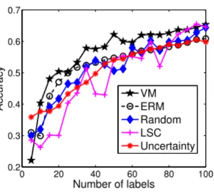
As can be observed from Fig. 3.1 to Fig. 3.3, our proposed VM algorithm significantly outperforms other active learning criteria on all the three data sets, especially when the number of labels is very small. LSC performs the second best on the Isolet and MNIST data sets when the number of labels is relatively small. It is interesting to note that on the MNIST data set, ERM

and Uncertainty perform not very well when the number of labels is small, and perform much better when more labels are selected, indicating that they rely heavily on the label information of

(36)

the selected data.

We further provide the detailed classification accuracy by using 20 and 50 labels in Table

3.1∼3.3. The last two columns of Table3.1and Table3.2record the average classification accuracy over different numbers of classes. We can see that overall, VM performs significantly better than all the other methods, including ERM and Uncertainty that use label information. Comparing with the algorithm that performs the second best in each case,VMachieves 27.0% (10.6%), 29.6% (6.2%), 6.4% (16.6%) relative error reduction in the average classification accuracy using 20 (50) labels on Isolet, MNIST and the co-author graph, respectively. We have also performed the two-tailed t-tests at 95% significance level over the experimental results in Table 3.1∼3.3. In all the cases thatVMperforms the best, thep-values between the results ofVMand other algorithms are less than 0.05. Therefore, the improvements of our proposed algorithm are statistically significant.

(37)

Chapter 4

Semi-Supervised Learning on

Heterogeneous Networks: A

Ranking-Based Classification

Approach

4.1 Overview

Semi-supervised classification is a critical problem in the field of semi-supervised learning. On heterogeneous networked data,semi-supervised classification(or classification in short) andranking

are two of the most fundamental analytical techniques. When label information is available for some of the nodes,classification makes use of the labeled data as well as the network structure to predict the class membership of the unlabeled data [66, 54]. On the other hand, ranking gives a partial ordering to nodes in the network by evaluating the node/link properties using some ranking scheme, such as PageRank [60] or HITS [40]. Both classification and ranking have been widely studied and found to be applicable in a wide range of problems.

Traditionally, classification and ranking are regarded as orthogonal approaches, computed in-dependently. However, adhering to such a strict dichotomy has serious downsides. Consider, for instance, an network of bibliographic data, consisting of some combination of published papers, authors, and conferences. As a concrete example, suppose we wish to classify the conferences in Table4.1into two research areas. We wish to minimize the chance that the top conferences are mis-classified, not only to improve our classification results overall, but also because misclassifying a top conference is very likely to increase errors on many other nodes that link to that conference, and are therefore greatly influenced by its label. We would thus like to more heavily penalize classification mistakes made on highly ranked conferences, relative to a workshop of little influence. Providing a ranking of all conferences within a research area can give users a clearer understanding of that field, rather than simply grouping conferences into classes without noting their relative importance. On

(38)

Table 4.1: Conferences from two research areas

Database SIGMOD, VLDB,

ICDE, EDBT, PODS, ... Information Retrieval SIGIR, ECIR,

CIKM, WWW, WSDM, ... Table 4.2: Top-5 ranked conferences in different settings

Rank Global Ranking Within DB Within IR

1 VLDB VLDB SIGIR

2 SIGIR SIGMOD ECIR

3 SIGMOD ICDE WWW

4 ICDE PODS CIKM

5 ECIR EDBT WSDM

the other hand, the class membership of each conference is very valuable for characterizing that conference. Ranking all conferences globally without considering any class information can often lead to meaningless results and apples-to-oranges comparisons. For instance, ranking database and information retrieval conferences together may not make much sense since the top conferences in these two fields cannot be reasonably compared, as shown in the second column of Table4.2. These kinds of nonsensical ranking results are not caused by the specific ranking approach, but are rather due to the inherent incomparability between the two classes of conferences. Thus we suppose that combining classification with ranking may generate more informative results. The third and fourth columns in Table 4.2 illustrate this combined approach, showing the more meaningful conference ranking within each class.

In this study, we propose RankClass, a new framework that groups nodes into several pre-specified classes, while generating the ranking information for each type of nodes within each class simultaneously in heterogeneous networked data. More accurate classification of nodes increases the quality of the ranking within each class, since there is a higher guarantee that the ranking algorithm used will be comparing only nodes of the same class. On the other hand, better ranking scores improve the performance of the classifier, by correctly identifying which nodes are more important, and should therefore have a higher influence on the classifier’s decisions. We use the ranking distribution of nodes to characterize each class, and we treat each node’s label information as a

(39)

prior. By building a graph-based ranking model, different types of nodes are ranked simultaneously within each class. Based on these ranking results, we estimate the relative importance or visibility of different parts of the network with regard to each class. In order to generate better within-class ranking, the network structure employed by the ranking model is adjusted so that the sub-network composed of nodes ranked high in each specific class is emphasized, while the sub-network of the rest of the class is gradually weakened. Thus, as the network structure of each class becomes clearer, the ranking quality improves. Finally, the posterior probability of each node belonging to each class is estimated to determine each node’s optimal class membership. Instead of performing ranking after classification, as facet ranking does [17,85], RankClass essentially integrates ranking and classification, allowing both approaches to mutually enhance each other. RankClass iterates over this process until converging to a stable state. Experimental results show that RankClass both boosts the overall classification accuracy and constructs within-class rankings, which may be interpreted as meaningful summaries of each class.

4.2 Problem Formalization

In this section, we introduce several related concepts and notations, and then formally define the problem.

Definition 1. Heterogeneous network. Given mtypes of nodes, denoted by X1 ={x11, . . . ,

x1n1}, . . . ,Xm = {xm1, . . . , xmnm}, a graph G = hV,E,Wi is called a heterogeneous network if

V =Sm

i=1Xi and m ≥ 2. E is the set of links between any two nodes of V, and W is the set of

weight values on the links. Whenm= 1, G reduces to a homogeneous network.

In the following sections, for convenience, we use X_i to denote both the set of nodes belonging to the i-th type and the type name. We letW_x_ip_x_jq denote the weight of the link between any two nodesxip and xjq, which is represented byhxip, xjqi.

In a heterogeneous network, each type of link relationship between two types of nodes Xi and

Xj can be represented by a relation graph Gij,i, j ∈ {1, . . . , m}. Note that it is possible fori=j.

LetRij be anni×nj relation matrix corresponding to graphGij. The element at thep-th row and

q-th column of Rij is denoted asRij,pq, representing the weight on link hxip, xjqi. There are many

(40)

definition is as follows: Rij,pq =     

1 if nodesxip and xjq are linked together

0 otherwise.

Here we consider undirected relation graphs such thatRij =RTji. In this way, each heterogeneous

networkG can be mathematically represented by a set of relation matrices G={Rij}mi,j=1.

To naturally generalize classification in homogeneous network data, we define a class in a het-erogeneous network to be a group of multi-typed nodes sharing a common topic. For instance, a research community in a bibliographic network contains not only authors, but also papers, venues and terms belonging to the same research area. Other examples include movie networks in which movies, directors, actors and keywords are tagged with the same genre, and E-commerce net-works where sellers, customers, items and tags belong to the same shopping category. The formal definition of aclass is given below:

Definition 2. Class. Given a heterogeneous network G = hV,E,Wi, V = Sm

i=1Xi, a class is

defined as G0 = hV0,E0,W0i, where V0 ⊆ V, E0 ⊆ E. ∀e = hxip, xjqi ∈ E0, where xip ∈ V0 and

xjq ∈ V0, we haveWx0ipxjq =Wxipxjq. Note here, V

0 _{also consists of multiple types of nodes from}

X₁ toX_m.

Definition 2 follows [75] and [39]. Notice that a class in a heterogeneous network is actually a sub-network containing multi-typed nodes that are closely related to each other. In addition to grouping multi-typed nodes into the pre-specified K classes, we also aim to generate the ranking distribution of nodes within each class k, which can be denoted as P(x|T(x), k), k = 1, . . . , K.

T(x) denotes the type of node x. Note that different types of nodes cannot be compared in a ranking. For example, it is not meaningful to create a ranking of conferences and authors together in a bibliographic network. Therefore, each ranking distribution is restricted to a single node type, i.e., Pni

p=1P(xip|Xi, k) = 1.

Now our problem can be formalized as follows: given a heterogeneous network G =hV,E,Wi, a subset of nodes V0 _{⊆ V} ₌ Sm

i=1Xi, which are labeled with values Y denoting which of the K

pre-specified classes each node belongs to, predict the class labels for all the unlabeled nodesV − V0 as well as the ranking distribution of nodes within each class, P(x|T(x), k),x∈ V,k= 1, . . . , K.

(41)

4.3 The RankClass Algorithm

In this section we introduce our ranking-based iterative classification method, RankClass. There are two major challenges when working with heterogeneous networks: (1) how to exploit the links representing the dependency relationships between nodes; and (2) how to model the type differences among nodes and links. The intuition behind RankClass is to build a graph-based ranking model that ranks multi-typed nodes simultaneously, according to the relative importance of nodes within each class. The initial ranking distribution of each class is determined by the labeled data. During each iteration, the ranking results are used to modify the network structure to allow the ranking model to generate higher quality within-class ranking.

4.3.1 The Framework of RankClass

We first introduce the general framework of RankClass. We will explain each part of the algorithm in detail in the following subsections.

• Step 0: Initialize the ranking distribution within each class according to the labeled data, i.e., {P(x|T(x), k)0}K

k=1. Initialize the set of network structures employed in the ranking model,

{G0

k}Kk=1, asGk0=G,k= 1, . . . , K. Initializet= 1.

• Step 1: Using the graph-based ranking model and the current set of network structures{G_kt−1}K k=1,

update the ranking distribution within each classk, i.e., {P(x|T(x), k)t}K k=1.

• Step 2: Based on{P(x|T(x), k)t}K

k=1, adjust the network structure to favor within-class ranking,

i.e., {Gt k}Kk=1.

• Step 3: Repeat steps 1 and 2, settingt=t+ 1 until convergence, i.e., until{P(x|T(x), k)∗}K k=1=

{P(x|T(x), k)t}K

k=1 do not change much for allx∈ V.

• Step 4: Based on {P(x|T(x), k)∗}K

k=1, calculate the posterior probability for each node, i.e.,

{P(k|x, T(x))}K

k=1. Assign the class label to node x as:

C(x) = arg max

1≤k≤K

(42)

4.3.2 Graph-based Ranking

Ranking is often used to evaluate the relative importance of nodes in a collection. In this work, we propose to rank nodes within their own type and within a specific class. The higher a node x

is ranked within class k, the more important x is for class k, and the more likely it is that x will be visited in class k. Clearly, within-class ranking is quite different from global ranking, and will vary throughout different classes.

The intuitive idea of our ranking scheme is authority propagation throughout the network. Taking the bibliographic network as an example, in a specific research area, it is natural to observe the following ranking rules [75]:

1. Highly ranked conferences publish many high quality papers. 2. High quality papers are often written by highly ranked authors.

3. High quality papers often contain keywords that are highly representative of the papers’ areas. The above authority ranking rules can be summarized as follows: nodes which are linked to-gether in a network are more likely to share similar ranking scores. Therefore, the ranking of each node can be iteratively updated by looking at the rankings of its neighbors. The initial rank-ing distribution within a class k can be specified by the user. When nodes are labeled without ranking information in a general classification scenario, we can initialize the ranking as a uniform distribution over only the labeled nodes:

P(xip|Xi, k)0 =      1/lik ifxip is labeled to class k 0 otherwise.

wherelik denotes the total number of nodes of typeXi labeled to classk.

Suppose the current network structure used to estimate the ranking within class k is mathe-matically represented by the set of relation matrices: G_kt−1 ={Rij}mi,j=1. For each relation matrix Rij, we define a diagonal matrixDij of sizeni×ni. The (p, p)-th element ofDij is the sum of the

(43)

construct the normalized form of the relation matrices as follows: Sij =D( −1/2) ij RijD (−1/2) ji , i, j∈ {1, . . . , m} (4.1)

This normalization technique is adopted in traditional graph-based learning [89] in order to reduce the impact of node popularity. In other words, we can suppress popular nodes to some extent, to keep them from completely dominating the authority propagation. Notice that the normalization is applied separately to each relation matrix corresponding to each type of link, rather than the whole network. In this way, the type differences between nodes and links are well-preserved [39]. At the t-th iteration, the ranking distribution of nodexip with regard to classk is

updated as follows: P(xip|Xi, k)t∝ Pm j=1λijSij,pqP(xjq|Xj, k)t−1+αiP(xip|Xi, k)0 Pm j=1λij +αi (4.2)

The first term of Equation (4.2) updates the ranking score of nodexip by the summation of the

ranking scores of its neighborsxjq, weighted by the link strengthSij,pq. The relative importance of

neighbors of different types is controlled byλij ∈[0,1]. The larger the value ofλij, the more value is

placed on the relationship between node typesXi andXj. For example, in a bibliographic network,

if a user believes that the links between authors and papers are more trustworthy and influential than the links between conferences and papers, then the λij corresponding to the author-paper

relationship should be set larger than that ofconference-paper. As a result, the rank of a paper will rely more on the ranks of its authors than the rank of its publication venue. The parameters λij

can also be thought of as performing feature selection in the heterogeneous network, i.e., selecting which types of links are important in the ranking process.

The second term learns from the initial ranking distribution encoded in the labels, whose contribution is weighted by αi ∈[0,1]. A similar strategy has been adopted in [49,39] to control

the weights between different types of relations and nodes. After each iteration, P(xip|Xi, k)t

is normalized such that Pni

p=1P(xip|Xi, k)t = 1, ∀i = 1, . . . , m, k = 1, . . . , K, in order to stay

consistent with the mathematical definition of a ranking distribution.