Contents lists available atScienceDirect
Computational Statistics and Data Analysis
journal homepage:www.elsevier.com/locate/csdaImproving cross-validated bandwidth selection using
subsampling-extrapolation techniques
Qing Wang
a,∗, Bruce G. Lindsay
baDepartment of Mathematics and Statistics, Williams College, Williamstown, MA, USA bDepartment of Statistics, Pennsylvania State University, University Park, PA, USA
h i g h l i g h t s
• A two-stage subsampling-extrapolation bandwidth selection procedure is proposed. • An automatic nested cross-validation method is developed to select the subsample size. • The extrapolated bandwidth selectors achieve a smaller mean square error.
• The second-order extrapolated bandwidth selector has a relative convergence rate n−1/4.
a r t i c l e i n f o
Article history:
Received 16 July 2013
Received in revised form 19 February 2015 Accepted 3 March 2015
Available online 16 March 2015
Keywords:
Bandwidth selection Cross-validation Extrapolation
L2distance
Nonparametric kernel density estimator Subsampling
a b s t r a c t
Cross-validation methodologies have been widely used as a means of selecting tuning parameters in nonparametric statistical problems. In this paper we focus on a new method for improving the reliability of cross-validation. We implement this method in the context of the kernel density estimator, where one needs to select the bandwidth parameter so as to minimizeL2risk. This method is a two-stage subsampling-extrapolation bandwidth
selection procedure, which is realized by first evaluating the risk at a fictional sample size
m(m≤sample sizen)and then extrapolating the optimal bandwidth frommton. This two-stage method can dramatically reduce the variability of the conventional unbiased cross-validation bandwidth selector. This simple first-order extrapolation estimator is equivalent to the rescaled ‘‘bagging-CV’’ bandwidth selector in Hall and Robinson (2009) if one sets the bootstrap size equal to the fictional sample size. However, our simplified expression for the risk estimator enables us to compute the aggregated risk without any bootstrapping. Furthermore, we developed a second-order extrapolation technique as an extension designed to improve the approximation of the true optimal bandwidth. To select the optimal choice of the fictional sizemgiven a sample of sizen, we propose a nested cross-validation methodology. Based on simulation study, the proposed new methods show promising performance across a wide selection of distributions. In addition, we also investigated the asymptotic properties of the proposed bandwidth selectors.
©2015 The Authors. Published by Elsevier B.V. This is an open access article under the CC BY-NC-ND license (http://creativecommons.org/licenses/by-nc-nd/4.0/).
1. Introduction
Cross-validation methodology has long been a popular method for selecting tuning parameters in non and semiparamet-ric models. However, it has also been criticized for its high variability and its corresponding tendency to overfit the data.
∗Correspondence to: 18 Hoxsey Street, Williamstown, MA 01267, USA. Tel.: +1 413 597 4960.
E-mail address:[email protected](Q. Wang). http://dx.doi.org/10.1016/j.csda.2015.03.005
0167-9473/©2015 The Authors. Published by Elsevier B.V. This is an open access article under the CC BY-NC-ND license (http://creativecommons.org/ licenses/by-nc-nd/4.0/).
This paper develops new methods for the improvement of the conventional cross-validation procedures. It is based on a blending ofU-statistic estimation and asymptotic theory. These new methods are realized by estimating the cross-validation risk with small training sets, then extrapolating the results to the desired sample size. The extrapolation step requires some asymptotic theory, but only the rate of convergence, not any unknown constants. We will show that such a two-stage procedure can dramatically reduce the high variability and overfitting that is the major liability of the conventional unbiased cross-validation.
We view our results as part of the following paradigm: when one is estimating nonparametrically a statistical property of samples of target sizem, such as the risk inherent in using a particular model, then one can do a much more accurate estimation when the targetmis much smaller than the actual sample sizen. The intuition is that there are many, many more subsamples of sizen
/
2, say, than there are subsamples of sizenorn−
1.To motivate our extrapolation methodology, we will here show how it works when used in risk estimation in the context of nonparametric kernel density estimation. In the process we will also show that for this problem the risk function for arbitrarymis surprisingly simple. In particular, cross-validation estimation at an arbitrary training sample size ofmdoes not require repeated subsampling at sizem, thereby greatly speeding up and improving accuracy of the methods we propose. We believe this to be a major new insight in the kernel density estimation literature.
To simplify notation, consider a univariate random variableX
∈
R. In statistical practice, we often know little about the underlying distribution ofXwhich is crucial in exploratory or inferential analysis (Silverman, 1986). So, our main task is to estimate the unknown density functionf(
x)
based on a set of observations. In this paper, we focus on the nonparametric kernel density estimator (Fix and Hodges, 1951). Given an i.i.d. sample of sizen,Xn=
(
X1, . . . ,
Xn)
, the kernel densityestimator atxis defined for a kernelKas
ˆ
fh(
x|
Xn)
=
n−1 n
i=1 Kh(
Xi−
x) (
x∈
R),
(1.1)whereh
>
0 is called the bandwidth parameter. HereKh(
t)
=
h−1K(
t/
h)
and functionKis the kernel function. As the choiceofKdoes not greatly affect the density estimation (Hardle et al., 1994), throughout this paper we consider a commonly used location kernel function, the Gaussian kernel.
Kh
(
x−
x0)
=
(
h√
2
π)
−1e−(x−x0)2/(2h2)∼
N(
x0
,
h2).
(1.2)However, our proposed methodologies do not depend on the choice ofK, and the theoretical results in this paper will be stated in terms of an arbitrary symmetric kernel functionKof orderr
(
r≥
2)
. For the definition of the order of a kernel function, please seeTurlach(1993).Although one has free choice of the kernel function in a density estimator, the choice of the bandwidthhis generally viewed as much more crucial. In order to select the optimal smoothing parameterh, we need to evaluate how closelyf
ˆ
hcanapproximateffor a given data set. Most bandwidth selectors are based on first choosing a risk function that measures the error made in using a particular bandwidthh. One can then estimate the risk function for a given data set and choose the bandwidth that minimizes the empirical risk. Such bandwidth selectors are referred to as data-driven methods.
The main result of this paper is to propose a two-stage subsampling-extrapolation bandwidth selection procedure. This work is closely related to the rescaled bagging cross-validation method ofHall and Robinson(2009) and the partitioned cross-validation method ofMarron(1987). Recent work involving bagging and subsampling in problems other than kernel density estimation includesMeinshausen and Buhlmann(2010) andShah and Samworth(2012). Unlike the bandwidth selectors discussed inPark and Marron(1990) andSheather and Jones(1991), which are based on asymptotic theory, our proposed methodology is a hybrid of the cross-validation method and the asymptotic theory. As such it does not require the estimation ofR
(
f′′)
or a third-stage estimation ofR(
f′′′)
. (By convention, we denoteR(
g)
=
g2
(
x)
dxfor any givenfunctiong.) Hence, it is more straightforward to implement than plug-in estimators. Most importantly, it can be used in a wide variety of problems where plug-in methodology is not available.
We present an extensive simulation study in Section4.1 to compare the proposed methods with the conventional cross-validation estimator. It will be seen that our bandwidth selectors achieve a smaller expected integrated square error that is much closer to the theoretical optimum than the standard cross-validation. Moreover, a comparison of the proposed methods to indirect cross-validation (Savchuk et al.,2011,2010;Mammen et al.,2012) can be found in Section4.2. In addition, we compare our methods to the asymptotic selection of the subsample sizemthat was described in
Marron(1987).
2. U-statistic estimate ofL2risk
In this section, we will derive a simple U-statistic form estimator for the risk that arises fromL2 distance. It is a
new representation for the unbiased risk estimator and enables us to calculate the aggregated risk at subsamples of size
m
(
m≤
n)
much more efficiently than the repeated bootstrapping done inHall and Robinson(2009) or the partitioning method used inMarron(1987).2.1. L2distance-based assessment
Define the integrated square error (ISE) as ISE
(
h)
=
ˆ
fh(
x|
Xn)
−
f(
x)
2 dx.
(2.1)If one wants to evaluatef
ˆ
hover all possible samples of sizen, one can consider the mean integrated squared error (MISE),also known as theL2risk.
RiskL2
(
h,
n)
=
MISE(
h)
=
EXn
ˆ
fh(
x|
Xn)
−
f(
x)
2 dx
.
(2.2)By Fubini’s theorem, the risk in(2.2)can be decomposed in the following fashion: RiskL2
(
h,
n)
=
EXn
{
f2(
x)
−
2f(
x)
fˆ
h(
x)
+ ˆ
fh2(
x|
Xn)
}
dx. Furthermore, one can omit terms independent ofhand focus on the relative risk, denoted asRL2(
h,
n)
=
−2
EXn{
f
(
x)
fˆ
h(
x|
Xn)
dx} +
EXn{
ˆ
fh2
(
x|
Xn)
dx}. It can be shown by simple algebra that the first expectation in
RL2(
h,
n)
can be represented asE{
Kh(
X1−
X2)
}. Moreover, the second expectation equals
E{
(
Kh∗
Kh)(
X1−
X2)
} +
n−1E{
(
Kh∗
Kh)(
0)
−
(
Kh∗
Kh)(
X1−
X2)
}, where
∗
is the convolution operator.If we denote
Ah
(
X1,
X2)
=
(
Kh∗
Kh)(
X1−
X2)
−
2Kh(
X1−
X2),
(2.3)Bh
(
X1,
X2)
=
(
Kh∗
Kh)(
0)
−
(
Kh∗
Kh)(
X1−
X2),
(2.4)then
RL2
(
h,
n)
=
E{
Ah(
X1,
X2)
} +
n−1E{
Bh(
X1,
X2)
}
.
(2.5) Note that theonlydependence on sample sizenon the right hand side of(2.5)occurs in the multipliern−1. In the caseof Gaussian kernel,
(
Kh∗
Kh)(
X1−
X2)
=
K√2h(
X1−
X2)
and(
Kh∗
Kh)(
0)
=
1/(
2h√
π)
. One can also denote MISE(
h)
as
bias2(
fˆ
h(
t))
dt+
Var
(
fˆ
(
t))
dt. Then,E{
Bh(
X1,
X2)
} =
n
Var
(
fˆ
h(
t))
dt corresponds to the integrated variance, andE
{
Ah(
X1,
X2)
} =
bias2
(
fˆ
h(
t))
dt−
f
(
t)
2dtis the relative integrated squared bias.Following the footsteps ofRay and Lindsay(2008) andLindsay and Liu(2009), we propose to estimate the risk at sample sizesmthat may be much smaller than the actual sizen. Ourm
<
nparadigm motivates us to hypothesize that these estimators will have much lower variability. Our simulations verify this. We also know that the cross-validation criterion for bandwidth selection tends to choose the bandwidths that are too small, and so overfit the density (Loader, 1999). As we will show, the new methodology particularly avoids the overfitting problem by reducing the chances of selecting a small bandwidth. Throughout this paper, we usemto represent the subsample size, which we might also call thefictional sample size. As we will see, it is closely related to the training sample size in cross-validation.Denote the relative risk evaluated at fictional sizemas
RL2
(
h,
m)
=
E{
Ah(
X1,
X2)
} +
m−1E{
Bh(
X1,
X2)
}
.
(2.6) This formula gives an important insight into the risk estimation problem. The only place the fictional sizemappears is as a coefficient. If we take the derivative ofRL2(
h,
m)
(2.6)with respect tohand set it equal to zero, we thereby identifyhas a potential minimum to the risk for thatm. We can invert this thinking and solveR′L2
(
h,
m)
=
0 withhfixed, thereby finding themthat leads to optimization of the risk.m∗
(
h)
= −
ddhE
{
Bh(
X1,
X2)
}
d
dhE
{
Ah(
X1,
X2)
}
.
(2.7)The uniqueness of the solution shows that for eachhthere is exactly onemfor which it is potentially optimal. In particular, ifKis the Gaussian kernel andfis the standard normal, we have
m∗
(
h)
=
{
(
h2
+
1)(
h2+
2)
}
3/2−
h3(
h2+
2)
3/22
√
2h3
(
h2+
1)
3/2−
h3(
h2+
2)
3/2.
(2.8)If we desire the optimalhfor a particular fixedm0, we solve the inverse problemm0
=
m∗(
hopt)
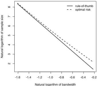
forhopt. This normal theory m∗ curve(2.8)will be examined later in light of the asymptotic theory (seeFig. 1). For now we note that in the normal examplem∗is decreasing inh. It follows that the optimal bandwidthhfor eachmis a decreasing function ofm.Remark 1. For difficult densities, the theoretical curvem∗
(
h)
is not monotonic, and so many methods based on asymptotics are likely to fail at some sample sizes. For example, if the curve has the shapev, with two regions of decrease separated by a region of increase, then for some values ofmthere will be three solutions inhtom=
m∗(
h)
. These will correspond to two local minima to the risk curve and the local maximum in-between. The central region in whichm∗(
h)
is increasing corresponds to values ofhthat are never optimal for any value ofm. For an example of this, seeFig. 6, where we show theFig. 1. Sample size against bandwidth whenfisN(0,1)on the log–log scale.
2.2. An unbiased estimate for L2risk
Because the relativeL2risk at fictional sizem,RL2
(
h,
m)
(2.6), involves the unknown density functionf, we cannot use it directly to find the optimal bandwidth. In practice, one needs to first estimate the risk based on a set of observations and then select an estimated optimal bandwidth by minimizing the estimated risk score. A straightforward (and unbiased) estimation forRL2(
h,
m)
is by constructing aU-statistic based on a kernel function of size two.Define UL2,m
=
n 2
−1
1≤i<j≤nψ
L2,h(
xi,
xj),
(2.9)where
ψ
L2,h(
x1,
x2)
=
Ah(
x1,
x2)
+
m−1Bh(
x1,
x2)
is a symmetric kernel function of size two, withAhandBhdefined earlierin(2.3) (2.4). Because a generalU-statistic is a function of the order statistics,UL2,m(2.9)therefore is the best unbiased
estimator for the relative risk in this nonparametric context (Fraser, 1954).
Note thatUL2,mis equivalent to the unbiased cross-validation formula whenm
=
n. That is, both of them are unbiased estimates for the relative MISE and are functions of the order statistics (modulo terms that do not depend onh). In addition, the un-rescaled bagging cross-validation bandwidth selector proposed byHall and Robinson(2009) is actually nothing more than the bandwidth selector based on(2.9)if one makes the bootstrap size equal tom. However, the simple expression for ourU-statistic risk estimator enables us to compute the aggregated risk much more efficiently than bootstrapping. First, we can generally compute the completeU-statistics, being of order two, much more efficiently than subsampling subsets of sizem. Secondly, the calculations can be done for allmat once, in effect.If we minimize(2.9)overhby setting the derivative inhto zero, we have
ˆ
m∗(
h)
= −
1≤i<j≤n d dhBh(
xi,
xj)
1≤i<j≤n d dhAh(
xi,
xj).
(2.10)This equation describes the dependence structure betweenmandhin minimizing the estimatedL2risk for a given sample of
sizen. In practice, one can construct aU-statistic form estimate for the risk at a fictional sample sizem. Then, by minimizing theU-statistic risk estimate one can obtain the optimal bandwidth choice for a given value ofm. We call this thesimple subsampling bandwidth selector. We note that the empirical curvem
ˆ
∗(
h)
is not necessarily strictly decreasing inh. If this happens, root selection rules must be applied.Remark 2. It is easy to plot the empirical curvem
ˆ
∗(
h)
for any particular data set. If the empirical curve is not monotonic decreasing in the region ofmvalues of interest, we would recommend against using extrapolation or plug-in methods.3. Bandwidth selection procedures
In this section we will examine several ways to usem
<
nrisk estimation to improve performance inL2risk minimization. They will proceed in order of increasing sophistication in their use of asymptotic theory.3.1. Using risk at m to select bandwidth
The simplest way to use the reduced variability of the risk estimator for smaller values ofmis to pick the bandwidthh
selected based onUL2,m
(
h)
. In addition to reducing variance inhestimation, however, one is introducing bias, and so one must consider the trade-off that occurs between bias and variance.We carried out a simulation study that indicated that asmdecreased the optimal bandwidthhmbecame larger (see
the 2012 Pennsylvania State University Ph.D. thesis of Q. Wang which is available electronically from Pennsylvania State University library). The average integrated square error decreased as one used fictional sizem
<
nuntilmreached a certain threshold, beyond which further improvement in MISE could not be achieved. For instance, in the standard normal case half-sampling withm=
n/
2 gave us the smallest simulated MISE, with an improvement of about 12% overm=
nfor samples of sizen=
100. This conclusion agrees with the result inHall and Robinson(2009).Although using a fictional sizem
<
ncan help to reduce the variability of the bandwidth selector and therefore achieve a smaller MISE, it turns out there are simple techniques to reduce this bias without increasing variance. We will show next in Section3.2how to do this.3.2. First-order extrapolation in selecting h
We now propose a two-stage, subsampling-extrapolation, approach in bandwidth selection. We will first develop a first-order extrapolated bandwidth selector. Motivated by the rule-of-thumb criterion, the two pieces we combine are the estimated optimal bandwidth atm
<
nand the rate of convergence of the estimator asn→ ∞
. Later we will offer further refinements to this method. We will then provide a simulation comparison of all methods.Recall theU-statistic form risk estimator,UL2,m(2.9), computed based on squared distance and evaluated at a fictional sample sizem. We denote the corresponding simple subsampling bandwidth selector ash
ˆ
L2,m, which minimizes theUrisk estimate at sizem. Althoughhˆ
L2,m(
m<
n)
was less variable thanhˆ
L2,n, it tended to be biased larger than the optimal bandwidth choicehoptat sample sizen. This is due to the fact thatm∗(
h)
(2.7)is decreasing inh, and we have evaluated therisk at a sizemless than the original sample sizen.
Our goal is to take advantage of the small variability of the risk estimate at fictional sizem
<
nand also try to remove the incurred bias inhˆ
L2,mby referring to the asymptotic relationship betweenmandhon the log–log scale. We can motivate our approach using the following well-known theory. If the densityf is known, the optimal bandwidth for minimizing the asymptotic MISE based on an order-2 kernel can be written ashopt
(
m)
=
m−1/5C(
f),
whereC
(
f)
is a constant depending onf. A typical rule-of-thumb bandwidth selector estimates the constantC(
f)
from the data in some way. For example, if we assume that both the true distribution and the kernel function are Gaussian, we then havehˆ
rot=
1.
06σ
ˆ
m−1/5, whereσ
ˆ
is an estimate for the population standard deviation.We have derived an explicit formula for findingm∗
(
h)
, the value ofmfor whichhis optimal. This asymptotic formula can be rearranged to say that, in the limit asmgets large, this relationship can be represented aslogm
=
C−
5 loghˆ
rot.
(3.1)HereCis a constant independent of the bandwidthh
ˆ
rot. This equation represents a straight-line relationship with slope−5
on the log–log scale. One may ask whether this simple linear relationship is a good approximation for the exact relationship between logm∗
(
h)
and loghfound in(2.7).Fig. 1displays the comparison between the rule-of-thumb criterion and the optimal risk criterion on the log–log scale when the underlying distributionfis the standard normal, and the kernel functionKis Gaussian. It can be seen that for a fixed value ofmthe rule of thumb always yields a smaller bandwidth than the one given by the exact risk curve, but their left hand asymptotes match.
Our derivation of(3.1)from the rule-of-thumb selection rule was heuristic. We therefore show more formally that this relationship is valid for any arbitrary smooth kernel functionKand density functionf. The following lemma verifies this statement. For proof, please seeAppendix.
Lemma 1. Assume K is a smooth symmetric kernel function of order r
(
r≥
2)
, and f is a probability density function that is(
2r−
1)
th order differentiable. By minimizing the L2risk, we can obtain the explicit expression of the fictional sample size m for which h would be optimal:m∗
(
h)
= −
ddhE
{
Bh(
X1,
X2)
}
d
dhE
{
Ah(
X1,
X2)
}
,
where Ah
(
x1,
x2)
and Bh(
x1,
x2)
are defined in(2.3)and(2.4). Moreover, it can be shown thatlogm∗
(
h)
+
(
2r+
1)
logh→
constant,
as h→
0.
And,
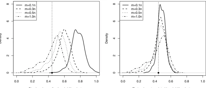
Fig. 2. Sampling distributions of simple subsampling and first-order extrapolated bandwidth selectors. The vertical dashed line marks the actual optimal bandwidth.
According toLemma 1, the optimal risk curve approaches the rule-of-thumb straight line on log–log scale as logh
→
−∞
. In particular, when one considers a Gaussian kernel, the order of the kernel functionris 2. In this case, we would havedlogm∗
(
h)/(
dlogh)
→ −5 as
h→
0. This confirms that the asymptotic slope of the optimal risk curve inFig. 1is indeed−5, the same as the slope of the rule-of-thumb straight line.
As a result, if one knows the bandwidth selected form, one simple way to remove the bias introduced by usingm
<
nis to extrapolate the bandwidth selected at sizemto the optimal value atnbased on the approximate linear relationship between logm∗and logh. We summarize the two-stage bandwidth selection procedure based on linear extrapolation as follows:
1. Subsampling stage: Construct theU-statistic estimate for the L2 risk at a fictional sizem
(
m≤
n)
and obtain thesubsampling bandwidth selector, denoted ash
ˆ
L2,m.ˆ
hL2,m
=
arg minh>0UL
2,m
(
h).
(3.2)2. Extrapolation stage: Extrapolateh
ˆ
L2,mto an approximation forhˆ
L2,nby referring to the approximate linear relationship between logm∗and loghas discussed inLemma 1. This gives the estimatorˆ
h1
=
(
m/
n)
1/5hˆ
L2,m.
(3.3)We callh
ˆ
1thefirst-order extrapolated bandwidth selector. Intuitivelyhˆ
1should have low bias whenmis close tonand when(
logh,
logm∗(
h))
relationship in minimizing theL2risk resembles a straight line. The fact thathˆ
1is a shrunken version of
ˆ
hL2,mmeans that it has less variance and so, as we shall see, the variability of the bandwidth selector is reduced significantly compared with the traditional cross-validation bandwidth selector.
For any particular densityf there will exist an optimal choice of the fictional sizemsuch that it optimizes the trade-off between bias and variance of the bandwidth selector.Fig. 2shows the density curves for the sampling distributions of the simple subsampling bandwidth selectorh
ˆ
L2,mand the first-order extrapolated bandwidth selectorhˆ
1at different fictional sample sizesm. These density curves were plotted based on drawingR=
500 samples of sizen=
100 from the standard normal distribution. This plot demonstrates graphically how the first-order extrapolation corrected for the bias incurred by usingm<
nwhile simultaneously reducing variability over standard cross-validation (m=
n). In particular, it greatly decreased the selection of values ofhthat were ‘‘too small’’, corresponding to overfitting. Later inTable 4it will be seen that the first order extrapolation improved the MISE efficiency ratio, MISEopt/
EISE(
hˆ
1)
, of the standard cross-validation from 64%to over 80%. Here EISE stands for expected integrated square error. The use of EISE rather than MISE in assessing bandwidth selectors was suggested byJones(1991). In our simulation section we will determine the optimal value ofp
=
m/
nfor a number of sampling distributions. It will be shown there that the optimal value of pvaries somewhat based on the smoothness of the density, butp=
0.
3 worked well for many. One possible strategy for the extrapolation estimator is to use a fixed value ofpregardless of the data. We will compare this strategy with a few others in the simulation section.3.3. Second-order extrapolation in selecting h
The first-order extrapolated bandwidth selector introduced in Section3.2is based on an approximate linear relationship between logm∗
(
h)
and logh. We have shown inLemma 1that the true optimal risk curve approaches the rule-of-thumb straight line ashgoes to 0. That is, the linear approximation is most accurate whenhis fairly small. Therefore, we wonder whether we could improve the approximation and seek a more accurate relationship between logm∗(
h)
and loghthat would be useful for smaller values ofn.Notice fromFig. 2that the first-order extrapolated bandwidth tends to be biased, more and more so as the range of extrapolation increases. As the optimal risk curve ofm∗
(
h)
is decreasing in h, we propose to consider a second-order correction. We start by noticing that the explicit expression form∗(
h)
can be written asm∗
(
h)
=
(
1/
2√
π)
h−2+
2hµ
2(φ)
C02+
o(
h)
4h3 C1+
6h5C2+
o(
h5)
,
whereµ
j(φ)
=
xj
φ(
x)
dxandφ
is a Gaussian kernel, andC ij=
f(i)
(
x)
f(j)(
x)
dxfori,
j∈
Zwith the assumption that
f(0)
(
x)
=
f(
x)
. In addition,C1
=
µ
4(
K)
C04/
24+
(µ
2(φ))
2C22/
8 andC2=
(
3/
96)µ
2(φ)µ
4(φ)
C24.To find the correct second order expansion, we need to take this expansion to the next term. We use the approximation log
(
1+
x)
≈
xforxclose to 0, and writelog
−
d dhE(
Bh(
X1,
X2))(
2h 2√
π)
=
log{1+
2h3µ
2(φ)
C02(
2√
π)
+
o(
1)
}
≈
2h3µ
2(φ)
C02(
2√
π)
log
d dhE(
Ah(
X1,
X2))(
4h 3 C1)
−1
=
log{
1+
(
3C2/
2C1)
h2+
o(
1)
}
≈
h2(
3C2/
2C1).
Therefore, the overall magnitude of the second-order error on the log scale ish2.
We then assume
m∗
(
h)
≈ ˜
m(
h)
=
C0h−5eah2,
(3.4)whereC0is a constant anda
∈
R. Note that the adjustment termeahgoes to 1 ash→
0 but is strictly bigger than 1 ifh>
0anda
>
0.We propose to approximate parameteraby matchingm∗
(
h)
andm˜
(
h)
at two values ofhand solving for the unknowns. Leth0andc0h0(
c0>
1)
be two chosen bandwidths. The two equationsm∗
(
h0)
=
C0h−5
0 e
ah0
m∗
(
c0h0)
=
C0(
c0h0)
−5ec0ah0then provide a way to solve for the unknown parametera. In particular,
ˆ
a=
1 h20(
c02−
1)
log
c05m ∗(
c 0h0)
m∗(
h 0)
≥
0.
Then, for any unknownh, formula(3.4)can be represented as
m∗
(
h)
=
m∗(
h0)
m∗(
h)
m∗
(
h0
)
≈
m∗(
h0) (
h/
h0)
−5eaˆ(h−h0):=
m∗∗(
h).
We propose to invert the curvem∗∗determined by the last approximation to estimate an optimal bandwidth for any particularmincludingm
=
n. We note that the inversion relationship can be expressed as an explicit correction to the log–log linear relationship.logm∗∗
(
h)
=
logm∗(
h0)
−
5(
logh−
logh0)
+ ˆ
a(
h2−
h20).
(3.5)As seen in(3.5),m∗∗is in fact just an exponential curve fitted through the two points
(
logh0,
logm∗(
h0))
and(
log(
c0h0),
logm∗
(
c0h0
))
and with slope−5.
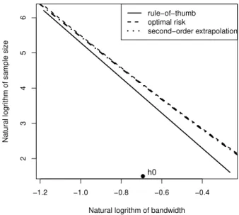
Fig. 3illustrates the theoretical curves of
(
logh,
logm(
h))
relationship whenf is the standard normal. The solid line isbased on the rule-of-thumb criterion; the dashed curve represents the exact relationship between logm∗
(
h)
and loghin minimizing theL2risk(2.8); the dotted curve displays the relationship of the second-order extrapolation based on formula(3.5), usingc0
=
2 andh0=
0.
5 as an illustration.It can be clearly seen that the second-order extrapolation curve was surprisingly close to the true optimal risk curve for the standard normal case. It should provide less bias than the first-order extrapolation, but it could add variability. In other words, we might expect the second-order extrapolation method to outperform the linear extrapolation bandwidth selector for cases where the density function is fairly smooth.
Fig. 3. Sample size against bandwidth on the log–log scale whenfis standard normal. Here,h0=0.5 as an illustration.
In our implementation of this second-order extrapolation in the simulation, we choseh0in(3.5)to be the subsampling
bandwidth selectorh
ˆ
L2,mat the fictional sizem=
pn. As a result,m∗(
h0)
≈
m. We also usedc0=
2, and estimatedm∗by using Eq.(2.10): m∗(
c0h0)
≈ ˆ
m∗(
c0hˆ
L2,m)
= −
1≤i<j≤n d dhBc0hˆL2,m(
Xi,
Xj)
1≤i<j≤n d dhAc0hˆL2,m(
Xi,
Xj)
.
Parameterawas then estimated byaˆ
= { ˆ
h2L2,m
(
c02−
1)
}
−1log{c5 0m
ˆ
∗
(
c0h
ˆ
L2,m)/
m}.
Under this scheme, given a sample of sizen, the optimal bandwidth atn, as extrapolated fromm
(
m<
n)
based on Eq.(3.5)is the root of the following score function, denoted ash
ˆ
2. We call it thesecond-order extrapolated bandwidth selector.logn
=
logm−
5
logh
−
loghˆ
L2,m
+ ˆ
a(
h2− ˆ
h2L2,m).
(3.6)Eq.(3.5)indicates thatm∗∗
(
h)
is bigger thanC0h−5, so we would expecth
ˆ
2to be smaller than the first-order extrapolationbandwidth selectorh
ˆ
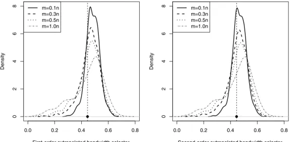
1for a given value ofm.To illustrate the advantage of the second-order extrapolation in comparison with the first-order extrapolation, we revisited the numerical study presented inFig. 2but now implemented the second-order extrapolation technique. InFig. 4
we compared the simulated density plots of the first-order and second-order bandwidth selectors when the fictional sample sizem
=
0.
1n,
0.
3n,
0.
5nor 1.
0n. It is clearly seen that for small values ofm, the improvement of the bandwidth selector based on second-order extrapolation is noticeable.3.4. Selecting the optimal fictional size: nested cross-validation
We will see in our simulation section that the optimal fictional size for both first and second-order extrapolation depends on the choice ofp
=
m/
n. In real problems one cannot determine the optimal choice of the fictional sizem=
pnthat minimizes the risk atn. As a result, when implementing the two-stage bandwidth selection procedure, one needs to either fix the choice ofmprior to bandwidth selection, or implement an automatic, data-driven method to pick the best choice ofmbased on a data set. Previous literature, such asHall and Robinson(2009),Shah and Samworth(2012), andShao(1993), suggest to usem
≤
n/
2. However, in their papers there does not exist an automatic selection method for picking the best choice ofmin the subsampling (or bagging) procedure. Here we propose a nested cross-validation methodology in selecting the optimal fictional sample sizemthat overcomes the drawback of choosing fictional sizemsubjectively. This method seems to perform consistently well across a wide selection of distributions (Section4.1). We note that this two-layer cross-validation is made computationally feasible by ourU-statistic estimation of the bandwidth selector curve.Letp
=
m/
nbe the fixed proportion of data used in the fictional sample. We consider a cross-validation strategy for selectingp. Letfˆ
p,n∗be the estimator of the density based on extrapolation (first or second-order) for a data set of sizen∗by subsampling of sizem=
pn∗. As we show below, from a sample of sizenwe can estimate theL2risk ofˆ
fp,n∗unbiasedly asFig. 4. Sampling distributions of first-order (left panel) and second-order (right panel) extrapolated bandwidth selectors whenfis Standard Normal. The vertical dashed line marks the actual optimal bandwidth.
a function ofpprovided thatn∗
<
n. We again acknowledge we will get more stable estimation whenn∗is not close ton, and so usen∗=
n/
2 in our simulation. We choose the value ofpthat minimizes the estimated risk at sizen∗. We then use this selected value ofpto create the extrapolation estimator on the full sample ofndata points.Denote the data set of sizenasXn
=
(
X1, . . . ,
Xn)
. We can take a random subsampleS of sizen∗<
n, say S=
(
X1∗, . . . ,
Xn∗/2)
withn∗=
n/
2, without replacement out ofXn. We then consider a grid ofpvalues, i.e.pj(
1≤
j≤
J)
.For each choice ofpand a subsampleS, one can realize the subsampling-extrapolation bandwidth selector by first finding the optimal bandwidth at sizepn∗and then extrapolating it frompn∗ton∗. We denote the extrapolated bandwidth at size
n∗ash
ˆ
p,S. Note thath
ˆ
p,Sis dependent on both the proportion choicepand the subsampleS.We want to consider theL2risk of using bandwidthh
ˆ
p,S at sample sizen∗as a function ofpand then determine the
optimal choice ofpat sizen∗. We denote the risk at sizen∗as
RL2
(
p,
n∗)
∝
E
ˆ
fp,n∗(
x)
2dx
−
2E
f(
x)
ˆ
fp,n∗(
x)
dx
,
(3.7) wherefˆ
p,n∗(
x)
=
n∗−1
n ∗i=1Khˆp
(
x−
Xi)
, andhˆ
pis the bandwidth extrapolated frompn∗ton∗.Since the density estimator
ˆ
fp,n∗(
x)
depends on both the random subsampleSand the choice ofp, the risk functionR(
p,
n∗)
cannot be estimated by the standardUestimator in(2.9). However, one can estimate the first expectation in(3.7)unbiasedly by
nn∗
−1
S
n∗−2
i
j(
Kˆhp∗
Khˆp)(
xi−
xj)
. The second expectation in(3.7)can be estimated unbiasedly by
n n∗
−1
S
(
n−
n∗)
−1
Xi̸∈Sˆ
fp,n∗(
Xi|
S)
,
whereSrepresents a subset of sizen∗taken out ofXn.In practice, one can repeatedly draw subsamples of sizen∗out ofX
n, denoted asS1
, . . . ,
SB. For a particular value ofp,we denote the first-order extrapolated bandwidth at sizen∗ash
ˆ
p,S1
, . . . ,
hˆ
p,SB. The estimated risk of using proportionpat sizen∗is thenˆ
RL2(
p,
n∗)
∝
1 B B
b=1
1 n∗2
i
j(
Khˆp, Sb∗
Kˆhp,Sb)(
xi−
xj)
−
2 B B
b=1
1 n−
n∗
Xi̸∈Sbˆ
fp,n∗(
Xi|
Sb)
.
(3.8)There exists a choice ofpthat minimizesR
ˆ
L2(
p,
n∗)
which is the optimal proportionpat sizen∗. We might hope that the bestpforn∗also yields satisfactory performance at sample sizen. If the optimal choice ofpdoes not largely rely on the subsample sizen∗, then it would be reasonable to identify the optimal choice ofpfornbased on a smaller sizen∗using the nested cross-validation methodology.Remark 3. Marron(1987) presents a method that is closely related to bagging cross-validation which he calls partitioned cross-validation. Marron (1987) shows that the proportion of subsample, p
=
m/
n, achieves its optimal value atTable 1
Density functions considered in the simulation study.
Distribution Probability density function Standard normal N(0,1) t(2) t(2) Mixture 1 0.5N(−1.5,1)+0.5N(1.5,1) Mixture 2 0.5N(0,1)+0.5N(0,0.1) Mixture 3 0.5N(0,1)+0.5N(0,0.01) Ten-fold mixture 0.110 i=1N(10i−5,1) Claw density 0.5N(0,1)+0.14 i=0N(i/2−1,0.01) pMarron
=
(σ /
C1)
−5/4n−3/8, where C1=
K2(
x)
dx
3/5
x4K(
x)
dx
(
f(2)(
x))
2dx
2
20
x2K(
x)
dx
11/5
(
f(2)(
x))
2dx
8/5
,
andσ
2=
8
(
f(
x))
2dx
[K∗
(
K−
L)(
x)
−
(
K−
L)(
x)
]2dx
25
K2(
x)
dx
7/5
x2K(
x)
dx
6/5
(
f(2)(
x))
2dx
3/5
.
Here, functionLis defined asL
(
x)
= −
xK′(
x)
, and∗
is the convolution operator. The constant
[
K∗
(
K−
L)(
x)
−
(
K−
L)(
x)
]
2dxin the definition of
σ
2can be obtained with the help of Corollary 6.4.1. inAldershof et al.(1995). We refer to Marron’sformula as MCV. Based on Marron’s formula,pgoes to zero asngoes to infinity. To compute the optimal partition size, one needs to estimate the integrated square derivatives of the unknown density function using two-stage estimators such as those proposed inJones and Sheather(1991). We will compare Marron’s formula with our nested cross-validation proposal through simulation studies in Section4.1.
4. Simulation studies
We have now developed four possible methods for bandwidth selection based on subsampling plus extrapolation: we have the first- and second-order extrapolations carried out at a fixed, pre-chosenp, plus the two extrapolation methods usingpchosen from a nested cross-validation. In order to investigate the performance of the proposed two-stage bandwidth selection procedures, we conducted the following simulation studies.
4.1. Comparison to unbiased cross-validation
We considerR
=
500 random samples of sizen(n=
100 or 200) drawn independently from a certain distribution. A list of the seven distributions under consideration can be found inTable 1, among which there are bimodal/multimodal, outlying, and heavy-tailed distributions. A particularly difficult density is the claw, with 5 extreme spikes, each with only 10% of the data. As we will see later inTable 4, it will create an outlier in our results. Other literature that consider the claw density and notice its unusual behavior includeMarron and Wand(1992) andLoader(1999).For each subset taken out ofXn, we consider ten possible values ofp
=
m/
n, i.e.p=
0.
1,
0.
2, . . . ,
1.
0. In selecting theoptimal choice ofp, we first compare the performance between the nested cross-validation withn∗
=
n/
2 and Marron’s formula (seeRemark 3). We compute percent of times eachpvalue is selected out of the 500 replications based on each method.Tables 2and3reveal that the selection ofpis quite noisy forn=
100, but does improve forn=
200. In making comparisons between the two methods, one should notice that Marron’s optimalpis not exactly the minimizer of Eq.(3.7)but the asymptotic minimizer of MSE
(
p)
=
E{
(
hˆ
p−
hMISE)
2}, with
hMISEbeing the minimizer of MISE. Regardless of thedifferent target functions for minimization, Marron’s formula has less variation than our nested method, and so might be expected to show somewhat better performance. We will investigate this point in our simulation section.
Next, we conduct an empirical investigation of how well one could estimate the optimalpusing a nested cross-validation withn∗
=
n/
2. The optimal proportionpopt,nthat is dependent on sample sizen, is the minimizer of Eq.(3.7)withn∗
=
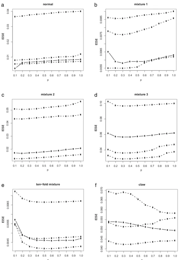
n.For several samples from each distribution, we plot the empirical expected integrated square error (EISE) curve as a function ofpbased on formula(3.8)in order to see whether we could do a good job at estimating the risk as a function ofp. InFig. 5
each of the panels displays three empirical curves (dashed curve) based on three random samples of sizen
=
100, taken from the corresponding distribution, and the theoretical true risk curve (solid curve) at sizen=
100. (The curves for t(2) distribution are omitted here, as they show similar pattern as in the normal case.) Although the empirical curves are quite variable, the shape of each curve seems to follow the truth in most of the cases except the claw density. Thus, we will use the nested cross-validation methodology in the following discussions.We then compare the performance of different bandwidth selectors in terms of the efficiency ratio, MISEopt
/
EISE(
hˆ
p)
,Table 2
Percentages of optimalpselections out ofR=500 replications.
R=500,n∗=
n/2 p=0.1 0.2 0.3 0.4 0.5 0.6 0.7 0.8 0.9 1.0
Standard normal
popt,n=0.1 Nested cross-validation (n=100)
Percent (%) 92.8 3.4 1.0 1.2 0.2 0.6 0.0 0.4 0.0 0.4
popt,n=0.1 Marron’s Formula (n=100)
Percent (%) 0.0 53.6 43.8 2.6 0.0 0.0 0.0 0.0 0.0 0.0
popt,n=0.1 Nested cross-validation (n=200)
Percent (%) 93.0 3.8 1.0 0.2 0.2 0.2 0.0 0.2 0.2 1.2
popt,n=0.1 Marron’s Formula (n=200)
Percent (%) 7.4 91.0 1.6 0.0 0.0 0.0 0.0 0.0 0.0 0.0
Mixture1
popt,n=0.3 Nested cross-validation (n=100)
Percent (%) 45.6 8.6 14.8 12.0 8.8 4.6 2.0 0.6 1.6 1.4
popt,n=0.3 Marron’s Formula (n=100)
Percent (%) 0.2 1.6 17.2 80.8 0.2 0.0 0.0 0.0 0.0 0.0
popt,n=0.3 Nested cross-validation (n=200)
Percent (%) 18.2 18.8 30.8 17.6 7.2 2.6 1.6 1.2 0.6 1.4
popt,n=0.3 Marron’s Formula (n=200)
Percent (%) 0.0 3.2 96.6 0.0 0.0 0.0 0.0 0.0 0.0 0.2
Mixture2
popt,n=0.2 Nested cross-validation (n=100)
Percent (%) 22.6 39.6 19.8 7.2 4.2 2.4 1.0 1.0 0.4 1.8
popt,n=0.2 Marron’s Formula (n=100)
Percent (%) 0.0 0.4 43.4 46.6 8.6 0.6 0.4 0.0 0.0 0.0
popt,n=0.2 Nested cross-validation (n=200)
Percent (%) 21.0 47.6 17.4 8.2 2.0 1.6 0.8 0.6 0.4 0.4
popt,n=0.2 Marron’s Formula (n=200)
Percent (%) 0.0 29.4 69.2 1.4 0.0 0.0 0.0 0.0 0.0 0.0
Table 3
Percentages of optimalpselections out ofR=500 replications.
R=500,n∗=
n/2 p=0.1 0.2 0.3 0.4 0.5 0.6 0.7 0.8 0.9 1.0
Mixture3
popt,n=0.3 Nested cross-validation (n=100)
Percent (%) 0.2 7.8 26.0 28.0 15.0 9.8 4.0 3.8 2.0 3.6
popt,n=0.3 Marron’s Formula (n=100)
Percent (%) 0.0 0.0 2.0 85.2 12.6 0.2 0.0 0.0 0.0 0.0
popt,n=0.2 Nested cross-validation (n=200)
Percent (%) 0.0 19.4 40.8 19.8 10.2 4.6 1.4 0.8 1.2 1.8
popt,n=0.2 Marron’s Formula (n=200)
Percent (%) 0.0 95.6 4.4 0.0 0.0 0.0 0.0 0.0 0.0 0.0
Claw density
popt,n=1.0 Nested cross-validation (n=100)
Percent (%) 72.2 10.6 4.2 1.8 0.8 0.4 1.0 0.4 0.8 7.8
popt,n=1.0 Marron’s Formula (n=100)
Percent (%) 0.0 0.0 0.6 3.2 11.4 32.0 36.2 10.8 5.4 0.4
popt,n=1.0 Nested cross-validation (n=200)
Percent (%) 32.6 10.0 2.8 0.2 0.0 0.2 1.4 1.6 5.0 46.2
popt,n=1.0 Marron’s Formula (n=200)
Percent (%) 0.0 0.0 1.4 14.4 55.0 24.0 5.2 0.0 0.0 0.0
Ten-fold
popt,n=0.6 Nested cross-validation (n=100)
Percent (%) 58.4 0.0 0.0 0.2 9.4 17.0 10.8 3.2 0.2 0.8
popt,n=0.6 Marron’s Formula (n=100)
Percent (%) 0.0 0.0 0.0 1.2 14.6 31.2 29.0 18.4 5.6 0.0
popt,n=0.4 Nested cross-validation (n=200)
Percent (%) 0.0 0.0 0.2 13.2 46.2 28.6 8.6 2.6 0.0 0.6
popt,n=0.4 Marron’s Formula (n=200)
a
b
c
d
e
f
Table 4
Comparison of efficiency ratio, MISEopt/EISE(hˆp), where the mixtures are in order of the cross-validation efficiency. Boldface indicates the best of the five competing methods.
n=100 CV EX1 EX2 EX1 EX2
MCV NCV Fixedp NCV Fixedp Optimalp Optimalp
Normal 63.7% 80.9% 81.5% 80.8% 84.1% 83.3% 87.4% 88.2% p=0.3 p=0.2 p=0.1 p=0.1 t(2) 69.8% 82.8% 80.5% 82.6% 81.1% 83.2% 84.5% 85.0% p=0.3 p=0.2 p=0.1 p=0.1 Mixture 2 68.5% 81.8% 79.5% 82.6% 83.5% 84.8% 84.4% 84.8% p=0.3 p=0.2 p=0.2 p=0.2 Mixture 1 78.7% 84.3% 84.8% 85.5% 80.6% 84.8% 85.5% 85.2% p=0.3 p=0.2 p=0.3 p=0.3 Mixture 3 80.1% 87.7% 87.8% 87.8% 88.2% 88.4% 87.5% 88.4% p=0.3 p=0.2 p=0.2 p=0.2 Ten-fold 94.3% 98.3% 86.9% 94.3% 94.4% 97.2% 96.3% 98.9% p=0.3 p=0.2 p=0.6 p=0.5 Claw 74.7% 72.9% 68.2% 68.5% 68.9% 68.8% 74.7% 74.7% p=0.3 p=0.2 p=1.0 p=1.0
MISE CV EX1 EX2 EX1 EX2
n=200 MCV NCV Fixedp NCV Fixedp Optimalp Optimalp
Normal 68.0% 86.6% 83.8% 83.8% 89.9% 86.1% 90.0% 90.0% p=0.3 p=0.2 p=0.1 p=0.1 t(2) 73.9% 86.2% 83.8% 86.3% 86.0% 86.7% 87.9% 88.5% p=0.3 p=0.2 p=0.1 p=0.1 Mixture 2 67.3% 86.3% 84.0% 86.1% 86.5% 87.4% 87.1% 88.5% p=0.3 p=0.2 p=0.2 p=0.1 Mixture 1 73.7% 88.6% 80.1% 93.3% 91.4% 89.1% 93.5% 89.5% p=0.3 p=0.2 p=0.4 p=0.3 Mixture 3 77.4% 87.1% 86.1% 87.1% 87.2% 87.8% 87.2% 87.8% p=0.3 p=0.2 p=0.2 p=0.2 Ten-fold 93.6% 98.8% 95.3% 95.3% 99.2% 99.5% 95.7% 99.6% p=0.3 p=0.2 p=0.4 p=0.4 Claw 82.1% 69.1% 61.7% 52.0% 48.4% 46.6% 82.1% 82.1% p=0.3 p=0.2 p=1.0 p=1.0
Wand(1992) to compute the theoretical optimal bandwidth for normal mixtures, and approximate the theoretical optimal bandwidth for t(2) by simulation. Notice that in practice without replication of size-nsamples, the optimal choice ofpat size
nis not obtainable. We first determine how the optimal choice ofpvaries over our sampling distributions. InTable 4EX1 and EX2 stand for first- and second-order extrapolations respectively. In the last two columns ofTable 4, one can see the relative efficiency ratio that can be attained when one uses the optimal value ofpfor that density. The optimalpseems to vary somewhat over the densities. One can also see that the second-order extrapolation, with optimalp, seems to do better than first-order extrapolation. After comparing the EISE over a grid of values ofp, we choose to usep
=
0.
3 for the fixed-pfirst-order extrapolation andp
=
0.
2 for the fixed-psecond-order extrapolation; these values seem to yield satisfactory results across a wide range of distributions.Then, we focus on the comparison between the four proposed bandwidth selectors, i.e. the first- and second-order extrapolated bandwidth selectors with pre-chosenpor with nested cross-validation, and the unbiased cross-validated bandwidth selector. In addition, we also include the comparison between Marron’s formula (seeRemark 3) and nested cross-validation in selecting the optimalpin the context of first-order extrapolation. BecauseMarron(1987) only focuses on the study of first-order extrapolation, the comparison between Marron’s optimalpand the nested cross-validation method is only fair for the first-order extrapolated bandwidth selectorh
ˆ
1. We use MCV to stand for Marron’s formula and NCV to standfor nested cross-validation. In formula(3.8)h
ˆ
pis set to be the first-order extrapolated bandwidth for EX1 and thesecond-order extrapolated bandwidth for EX2. The realization of the second-second-order extrapolated bandwidth selector is based on settingh0
= ˆ
hL2,mandc0=
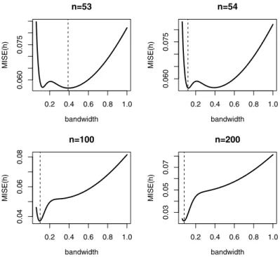
2.Our first observation fromTable 4is that the results from the claw density are distinctly different from the rest. This density is considered inLoader(1999) to demonstrate that plug-in methodologies could perform very poorly relative to conventional cross-validation.Van Es(1992) shows that the relative rate of convergence of ordinary cross-validation bandwidth selector is faster for non-smooth cases, such as in the case of claw density. It is noted inMarron and Wand
(1992) that the true MISE curve of the claw density has local minima when the sample sizen
≤
53 (seeFig. 6). That is,m∗(
h)
function has thevshape in the region ofmof interest as seen inFig. 7. It is clear from this plot why extrapolation of this curve can work so poorly at some sample sizes. Only whennincreases to above 100, does the MISE curve start to have an obviousFig. 6. The theoretical curve of MISE(h) for claw density at different sample sizesn. The dashed line in each panel marks the global minima of MISE(h).
Fig. 7. The theoretical and extrapolated curves ofm∗(
h)in the case of claw density on the log–log scale. The extrapolated point for the first-order extrapolation ish0 = 0.1 (−2.3 on log scale); the extrapolated points for the second-order extrapolation ish0 =0.1 and 0.2 (−2.3 and−1.6 on log
scale).
global minima. In this example, we have found that the efficiency ratio for the plug-in bandwidth selector ofSheather and
Jones(1991) is as small as 9.9% forn
=
100 and 6.1% forn=
200. Our extrapolation methods do perform much better thanplug-in methods in the case of claw density. Moreover, a user who follows our advice not to use extrapolation methods or plug-in whenm
ˆ
∗(
h)
is non-monotonic in the region of interest would end up using conventional cross-validation most of the time.If we ignore the claw density, we can make the following general observations: If we compare the methods that use first-order extrapolation, it is clear that for both sample sizesn
=
100 andn=
200, the fixed-pmethod yields slightly betterTable 5
Comparison to indirect cross-validation based onEˆ{ISE(hˆ)/ISE(hˆ0)}.
Standard normal
n UCV ICV EX1 EX2
fixedp=0.3 opt.p=0.1 fixedp=0.2 opt.p=0.1
100 2.4670 1.7218 1.6478 1.4171 1.7018 1.4434
n UCV ICV EX1 EX2
fixedp=0.3 opt.p=0.1 fixedp=0.2 opt.p=0.1
250 1.9159 1.4757 1.4637 1.3062 1.4186 1.3238
Bimodal normal mixture
n UCV ICV EX1 EX2
fixedp=0.3 opt.p=0.3 fixedp=0.2 opt.p=0.3
100 1.6995 1.3614 1.3667 1.3667 1.3827 1.3640
n UCV ICV EX1 EX2
fixedp=0.3 opt.p=0.3 fixedp=0.2 opt.p=0.2
250 1.5160 1.2874 1.2453 1.2453 1.2331 1.2331
results than nested cross-validation. The performance of Marron’s formula is similar to our proposed nested cross-validation in the context of first-order extrapolation at sample sizen
=
100, but MCV shows a small systematic superiority over NCV atn
=
200. However, the realization of Marron’s formula involves complex formulas as defined inRemark 3. Overall, we could obtain over 80% efficiency in all cases. The fixed-psecond-order extrapolation is almost a clear winner over the fixed-p first-order extrapolation. Moreover, the nested cross-validation using second-first-order extrapolation gives very similar performance as the fixed-psecond order extrapolation. Both seem promising bandwidth selection tools.In conclusion, we note that fixed-pfirst-order extrapolation is a computationally inexpensive way to improve upon standard cross-validation whenm∗
(
h)
is reasonably behaved. For additional refinements, one can apply the second-order extrapolation.4.2. Comparison to indirect cross-validation
Savchuk et al. (2011,2010)andMammen et al.(2012) discuss a modification of the unbiased cross-validation (UCV)
method, calledindirect cross-validation(ICV), that aims to reduce the large variability of UCV bandwidth selector with the help of a selection kernel.
Given a selection kernel of the following form
L
(
u;
α, σ )
=
(
1+
α)φ(
u)
−
α
σ
φ(
u/σ),
indirect cross-validation is to first find the UCV bandwidth selector based onL, sayh
ˆ
L, and then rescale it to a bandwidthusing Gaussian kernel
φ
. We denote the latter bandwidth selector ashˆ
φ. They argue that the conventional cross-validation works more stably with a more complicated kernel function than a second-order Gaussian kernel in bandwidth selection. The relationship betweenhˆ
Landhˆ
φis approximated based on expressions of their asymptotic optimal bandwidth, whichcan be written as
ˆ
hφ=
R(φ)µ
2 2L R(
L)µ
2 2φ
1/5ˆ
hL,
where the rescaler only depends on the selection kernel.
Following a referee’s suggestion, we will show below a numerical comparison between our proposed subsampling-extrapolation bandwidth selectors and the ICV bandwidth selector. To be comparable to the results inSavchuk et al.
(2011,2010), we consider the same simulation setting and choices of distribution functions: we considerR
=
1000independent samples of sizen(n
=
100 and 250) generated randomly from standard normal or a bimodal normal mixture 0.
5N(
−
1,
4/
9)
+
0.
5(
1,
4/
9)
. Notice that their bimodal normal mixture is essentially the same as our Mixture 1 showninTable 1. In addition, we computeE
ˆ
{
ISE(
hˆ
)/
ISE(
hˆ
0)
}
as the measure to evaluate the performance of each method. Thismeasure is used inSavchuk et al. (2011,2010)to evaluate the performance of the ICV bandwidth selector. It can be seen
inTable 5that our proposed bandwidth selectors perform comparably, or even better, than the indirect cross-validation
bandwidth selector.
Remark 4. Although indirect cross-validation bears similarity with our subsampling-extrapolation method, we use