Security proof methods for quantum key distribution protocols

(1)

Security proof methods for quantum

key distribution protocols

by

Agnes Ferenczi

A thesis

presented to the University of Waterloo in fulfillment of the

thesis requirement for the degree of Doctor of Philosophy

in Physics

Waterloo, Ontario, Canada, 2013

c

(2)

I hereby declare that I am the sole author of this thesis. This is a true copy of the thesis, including any required final revisions, as accepted by my examiners.

I understand that my thesis may be made electronically available to the public. A. Ferenczi

(3)

Abstract

In this thesis we develop practical tools for quantum key distribution (QKD) security proofs. We apply the tools to provide security proofs for several protocols, ranging from discrete variable protocols in high dimensions, protocols with realistic implementations, measurement device independent QKD and continuous-variable QKD. The security proofs are based on the Devetak-Winter security framework [31,57].

In the key rate calculation, it is often convenient to assume that the optimal attack is symmetric. Under the assumption that the parameter estimation is based on coarse-grained observations, we show that the optimal attack is symmetric, if the protocol and the postselection have sufficient symmetries. As an example we calculate the key rates of protocols using 2, d and d+ 1 mutually unbiased bases in d-dimensional Hilbert spaces.

We investigate the connection between the optimal collective eavesdropping attack and the optimal cloning attack, in which the eavesdropper employs an optimal cloner to attack the protocol. We find that, in general, it does not hold that the optimal attack is an optimal cloner. However, there are classes of protocols, for which we can identify the optimal attack by an optimal cloner. We analyze protocols with mutually unbiased bases ind dimensions, and show that for the protocols with 2 andd+ 1 mutually unbiased bases the optimal attack is an optimal cloner, but for the protocols with d mutually unbiased bases, it is not.

In optical implementations of the phase-encoded BB84 protocol, the bit information is usually encoded in the phase of two consecutive photon pulses generated in a Mach-Zehnder interferometer. In the actual experimental realization, the loss in the arms of the Mach-Zehnder interferometer is not balanced, for example because only one arm contains a lossy phase modulator. Since the imbalance changes the structure of the signals states and measurements, the BB84 security analysis no longer applies in this scenario. We provide a security proof for the unbalanced phase-encoded BB84. The loss does lower the key rate compared to a protocol without loss. However, for a realistic parameter regime, the same key rate is found by applying the original BB84 security analysis.

Recently, the security of a measurement device-independent QKD setup with BB84 signal states was proven in Refs. [61,14]. In this setup Alice and Bob send quantum states to an intermediate node, which performs the measurement, and is assumed to be controlled by Eve. We analyze the security of a measurement device-independent QKD protocol with B92 signal states, and calculate the key rates numerically for a realistic implementation. Based on our security proof we were able to prove the security of the strong reference pulse B92 protocol.

(4)

We analyze the security of continuous-variable protocols using the entropic uncertainty relations established in Ref. [11] to provide an estimate of the key rate based on the observed first and second moments. We analyze a protocol with squeezed coherent states and the 2-state protocol with two coherent states with opposite phases.

(5)

Acknowledgements

First and foremost, I want to thank my supervisor Norbert L¨utkenhaus, who gave me the opportunity to complete my Ph.D. thesis at the Institute for Quantum Computing. I especially want to thank for his support, advice and guidance that made this project possible. I am grateful for the opportunities he provided to visit international conferences and to spend a term abroad at the Max Planck Institute for the Science of Light in Erlangen. I would also like to thank the members of my advisory committee, Raymond Laflamme, Michele Mosca and David Kribs, for the thought-provoking questions during my advisory committee meetings, and to Mark Hillery for agreeing to be my external examiner.

Thanks to my colleagues in the OQCT research group for their helpful discussions and their friendship: Razieh Annabestani, Juan Miguel Arrazola, Normand Beaudry, Oleg Gittsovich, Hauke H¨aseler, Matthias Heid, Nathan Killoran, Xiongfeng Ma, Will Matthews, Sergei Mikheev, Tobias Moroder, Geir Ove Myhr, Varun Narasimhachar, Marco Piani, David Pitk¨anen, Mohsen Razavi and William Stacey.

Waterloo has become my new home, because of the many great friends who were a source of laughter, joy and support. Thanks to Varun and Razieh for sharing jokes that made me laugh so hard it hurt. Thanks to Jean-Luc, who has been a great roommate and friend. Thanks to my training partner, Florian, for the rides to triathlon and running races. Thanks to Jonathan for the scotch and beers. Thanks to Norm for the countless board game nights. Thanks to my office mates, Gina and Peter, for the interesting discussions.

Thanks to my friends at the runner’s choice marathon group, the Health and Perfor-mance group and the UW triathlon club for sharing the pain of countless training hours and for the encouragements to “never give up”.

Finally, I want to thank my family for their love, their constant encouragement and support.

(6)

List of Tables

2.1 The character table of the Dihedral Group D4 . . . 21

2.2 The character table of the Cyclic Group C4. . . 22

(12)

List of Figures

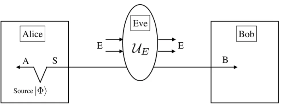
3.1 Source-replacement scheme . . . 32

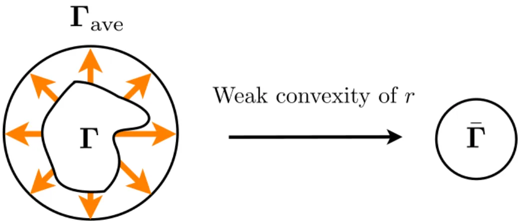
4.1 Set of symmetric attacks . . . 46

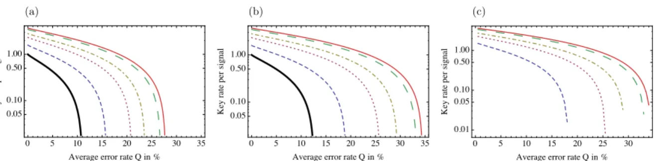
4.2 Key rates of the Pauli-MUB protocols. . . 58

4.3 Protocol with the same optimal attack as the 6-state protocol . . . 61

4.4 Protocol with the same optimal attack as the BB84 protocols. . . 62

5.1 Comparison between optimal cloner and optimal attack for the protocol with d Pauli MUBs . . . 70

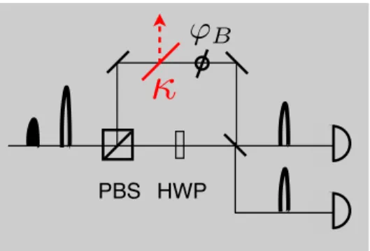
6.1 Phase-encoded BB84 setup . . . 74

6.2 Polarizing beam splitter protocol . . . 75

6.3 Lossless interferometer picture . . . 76

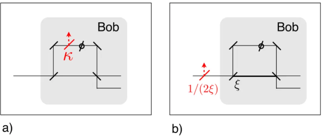
6.4 Hardware fix with additional loss . . . 77

6.5 Hardware fix with uneven beamsplitter . . . 77

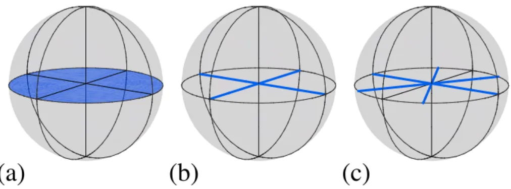
6.6 Signal states of the unbalanced phase-encoded BB84 protocol on the Bloch sphere . . . 80

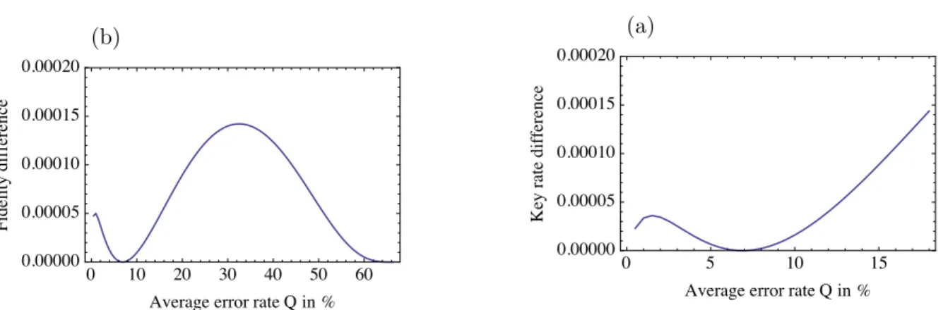
6.7 Key rates of the unbalanced phase-encoded BB84 protocol in dependence of the error rate . . . 87

6.8 Squashing map . . . 89

6.9 Key rates of the unbalanced phase-encoded BB84 protocol in dependence of the distance . . . 91

(13)

6.11 Comparison of different security proof methods . . . 93

7.1 MDI-B92 setup in the two-party source-replacement scheme. . . 98

7.2 Implementation of the optimal joint USD . . . 103

7.3 Key rate plots for MDI-B92 protocol . . . 112

7.4 Key rate plots for MDI-B92 protocol . . . 113

7.5 Probability distribution of a homodyne measurement in the node . . . 114

7.6 Setup of the strong reference pulse scheme. . . 115

7.7 Steps leading from the SRP scenario to the MDI scenario. . . 116

8.1 Key rates under beamsplitter attack on the 2-state protocol . . . 132

8.2 Comparison of the key rate based on the uncertainty principle and the Devetak-Winter formula . . . 133

(14)

Chapter 1 Introduction

The field of quantum cryptography including the subfield quantum key distribution emerged through the need to provide unconditionally secure communication protocols. The security of commonly used classical cryptography systems relies on concepts such as computational hardness of mathematical problems. Factoring a large number into the prime components is one such example, which is also the underlying security assumption of the classical cryp-tographic system RSA. With the emergence of Shor’s factoring algorithms, such classical cryptographic systems are threatened to be broken in reasonably short time. Although the practical implementation of Shor’s algorithm using a quantum computer is still in its infancy, it is necessary to start to build a defence system based on QKD before a quantum computer is ready to break existing cryptographic systems.

The goal of QKD is to enable two distant parties to generate a secret key by means of quantum mechanical principles. A secret key is a string of random bits known to both parties, but unknown to any third party. The secure key is later used to enable secure communication, message authentication or other cryptographic applications. QKD does not impose any computational limitations on an eavesdropper. If we accept quantum mechanics as a valid description of nature, then, in principle, unconditional security of the secret key can be guaranteed by QKD.

The process that generates the key, called protocol, is a predefined series of steps ex-ecuted by the two parties. In a QKD protocol, the sender, Alice, encodes random bits into nonorthogonal quantum states in her laboratory. She sends the states one by one through a quantum channel to the receiving party, Bob, who performs a measurement in his laboratory to obtain the encoded data. Finally, by means of classical communication protocols over an authenticated classical channel, Alice and Bob extract the secret key

(15)

from their data. Typically it is assumed that Alice and Bob’s laboratories are private, but the quantum channel and the classical channel are not. While the quantum states travel through the quantum channel, they are vulnerable to any interaction by a third party, the eavesdropper, Eve, whose aim is to learn about the key. Eve can also listen to all classical messages exchanged between Alice and Bob, but she can not change them.

A fundamental question is how to guarantee that in the end of the protocol the key is really safe to use in later applications. The basic intuition behind the security of a QKD protocol is based on the no cloning theorem, which states that it is not possible to make perfect copies of unknown quantum states. This theorem excludes the possibility that Eve intercepts the quantum channel, makes a perfect copy of the quantum states for herself, and forwards the original copies to Bob. Such a strategy would provide Eve with some knowledge about the encoded bit, without Alice and Bob noticing. Instead, Eve’s interaction (attack) with the signals does not go unnoticed by Alice and Bob. There is a trade-off between the amount of information that leaks to Eve and the amount of disturbance she causes to the signal states. This disturbance is observed by Alice and Bob in their data, which allows them to infer that an eavesdropper interacted with the signals. The main goal of a security proofs is to quantify the amount of information Eve obtains in the trade-off. Security proofs were given based on information-theoretic arguments by Devetak and Winter [31] or Renner, Kraus and Gisin [80, 57]. These proofs basically provide a bound on the amount of data that must be sacrificed in order to cut out Eve’s knowledge in the classical communication protocols. Furthermore, it is also necessary for Alice and Bob to make their classical data strings uniformly distributed and correct errors. The cost of this task also shortens the length of the final key.

Alice and Bob’s observations rarely identify the eavesdropping attack unambiguously. For most protocols (including the BB84 protocol) there is an entire class of eavesdropping strategies that can lead to the observed data. For each of the possible eavesdropping strategies, the Devetak-Winter security proof predicts a key rate. In order for Alice and Bob to be safe, they must protect themselves against the most powerful eavesdropping strategy. They must pick the smallest of the key rates, which is essentially the result of an optimization of the key rate over all possible attack strategies. The optimal eavesdropping strategy is therefore defined as the strategy that creates the smallest key rate among the class of strategies that fit to the observed data.

The primary goal of this thesis to advance the practical techniques used in the key rate optimization based on the Devetak-Winter security proof. In particular, we show how to exploit the underlying symmetries of a protocol in order to make the optimization problem simpler. This motivates us to provide explicit key rate calculations for a range of protocols

(16)

and scenarios: from highly theoretical protocols, such as the protocols using mutually unbiased bases in d-dimensional Hilbert spaces, to experimentally implemented protocols, such as the phase-encoded BB84 with realistic devices, to rather unusual setups, such as measurement device independent QKD with two senders and one adversary receiver.

Furthermore, we investigate the connection between the optimal eavesdropping strategy and the optimal cloning strategy. One type of eavesdropping strategy for Eve is to use an optimal quantum cloner, which makes the best possible copy of the signal states for her, while limiting the amount of disturbance in Bob’s copy to match his observations. It is known that for the BB84 and the 6-state protocol the optimal cloning strategy is the optimal eavesdropping strategy, but for other protocols this connection is not established. We investigate under what conditions and for which protocols the optimal eavesdropping strategy is identical with the optimal cloning strategy.

Finally, we explore new tools with the aim to tackle protocols, for which optimal security solutions have not been derived so far. These tools are based on measurement device-independent QKD and the entropic uncertainty relation.

This thesis is organized as follows: In Chapter2 we review the basic elements of quan-tum mechanics and representation theory that will be used later in the thesis. Chapter 3 is a summary of theoretical aspects of QKD: we describe the eavesdropping attacks in the source-replacement scheme, the Devetak-Winter key rate formalism under postselec-tion, and the key rate optimization problem. Chapters 4 to 8 contain the results of our research. In Chapter 4 we show that, under certain conditions, the optimal attack carries a certain symmetry inherent to the protocol. The symmetries are helpful for the practical calculation of the key rates. In Chapter 5 we analyze the connection between the optimal eavesdropping and the optimal cloning transformation. Chapter 6 is devoted to proving the security of the unbalanced phase-encoded BB84 protocol taking into account the lossy phase modulator. This protocol differs from the BB84 protocol, because the effect of a lossy phase modulator changes the signal and measurement structure. In Chapter 7 we provide a security proof for a measurement device-independent QKD setup with B92 signal states, where Alice and Bob are both senders of quantum signals, and Eve is the receiver. This security proof acts as a new security proof technique for the strong reference pulse B92. In Chapter 8, we use an entropic uncertainty relation with the aim to prove the security of continuous-variable protocols. Finally, in Chapter 9 we draw the conclusions.

(17)

Chapter 2 Background

2.1 Postulates of quantum mechanics

In this section we review the postulates of quantum mechanics with a focus on information theory [76, 73, 84].

2.1.1 Quantum states

Apure quantum state is defined as normalized vector Ψ on a d-dimensional Hilbert space H. In the Dirac notation the vector is represented by the symbol _|Ψ_i, which is called a

ket. The dual Hilbert space carries the vectors _hΨ_|=_|Ψ_i† where the symbol_†denotes the Hermitian conjugate. The inner product _hΨ_|Φ_i of two vectors _|Ψ_i,_|Φ_{i ∈ H} is identified with a scalar in C. The outer product _|Ψ_ihΦ_| of two vectors _|Ψ_i,_|Φ_{i ∈ H} defines a linear mapping from _H to itself, i.e. an endomorphism on _H. We denote the set of all endomorphisms on_H by _B(_H).

Definition 1 A density operatorρ_{∈ B}(_H)is a Hermitian, normalized and positive semidef-inite operator, i.e. ρ† = ρ, trρ = 1 and ρ_≥ 0. The set of all density operators on _H are defined as _D(_H).

Not all quantum states are pure states. For example, we might be interested in a statistical mixture of pure states_|Ψxiwith probabilityp(x), called an ensemble, or we might

(18)

are generally not pure. The first postulate of quantum mechanics defines general quantum states:

Postulate 1 Density operators provide a general mathematical description of quantum states. Pure states are represented by projectors ρ=_|Ψ_ihΨ_|. Quantum states that are not pure are called mixed states.

The density operator of the ensemble mentioned above is given by

ρ=X

x

p(x)_|ΨxihΨx|. (2.1)

Since a density operatorρ is Hermitian, there is an eigenvalue decomposition

ρ=

d

X

i=1

λi|φiihφi| (2.2)

with eigenvaluesλi and eigenvectors |φii.

If we define an orthonormal basis_{|i_i, i= 0, ..., d_}of a finite-dimensional Hilbert space, a quantum stateρ_{∈ D}(_H) can be expressed in that basis by

ρ=X

i,j

ai,j|iihj| (2.3)

with complex coefficients ai,j =hi|ρ|ji. If the quantum state is pure, then |Ψi =

P

ici|ii

with complex coefficientsci =hi|Ψi.

Qubits and Pauli operators

Aqubit is a quantum state defined on a two-dimensional Hilbert space_H2. The word qubit

is a concatenation of the words ‘quantum’ and ‘bit’. Qubits are the most suitable choice to represent a quantum analogue of the classical ‘bit’. Therefore, thecanonical basis (also called computational basis or standard basis) is typically denoted by the two normalized vectors_|0_i and _|1_iin analogy to the classical bits 0 and 1.

An important set of operators on_H2are the Pauli operators ˆσx, ˆσy and ˆσz, or sometimes

denoted byX,Y andZ. Together with the identity operator ˆσ0 ≡1, they span an operator

(19)

Definition 2 The Pauli operators are Hermitian, positive and unitary. In the computa-tional basis _{|0_i,_|1_i}, they are expressed by

ˆ σx =|0ih1|+|1ih0| (2.4) ˆ σy =−i|0ih1|+i|1ih0| (2.5) ˆ σz =|0ih0| − |1ih1|. (2.6)

Any state ρ on the qubit Hilbert space is conveniently represented in the Bloch repre-sentation

ρ= 1

2(1+~s·~σ) (2.7)

where ~σ = (ˆσx,σˆy,σˆz) is a vector of Pauli operators. The vector ~s = (sx, sy, sz) is called

Bloch vector with real coefficients si with the property|~s|2 =s2x+s2y+s2z ≤1. The vector

~

s defines a representation of a qubit on the three-dimensional real sphere known as Bloch sphere. All pure states lie on the surface of the sphere with_|~s_|2 _{= 1.}

2.1.2 Composite systems

Individual quantum systems can be joined to form a composite quantum system. The second postulate of quantum mechanics defines joint systems.

Postulate 2 Let us denote the Hilbert spaces corresponding to the systemsA andB by_HA

and_HB. Then the joint space is given by the tensor product Hilbert spaceHAB =HA⊗HB.

Quantum states of joint systems are denoted by density operatorsρAB in D(HAB).

Perhaps we are only interested in one subsystem of a joint stateρAB. The state reduced

to one subsystem is defined as follows.

Definition 3 Let ρAB ∈ D(HAB). The reduced state ρA of ρAB on the subsystem A is

obtained by taking the partial trace over the system B

ρA= trB{ρAB}. (2.8)

Similarly, the the partial trace over A results in a reduced state ρB = trAρAB on the

(20)

If the individual subsystems of a joint state ρAB are independent, the state is said to

be a product state.

Definition 4 A state ρAB is said to be a product state if it is of the form ρAB =ρA⊗ρB.

A pure state _|Ψ_iAB is said to be a product state if it is of the form |ΨiAB =|ΨiA⊗ |ΨiB.

For example, suppose_{|iAi}i and {|jBi}j are two orthonormal bases of the Hilbert spaces

HA and HB. One choice of a basis for the joint system HAB is a product basis with the

basis vectors_|iAi ⊗ |jBi ≡ |iA, jBi.

A unique quantum mechanical feature of composite systems isentanglement. Entangle-ment is a resource that plays a fundaEntangle-mental role in quantum communication and quantum computation.

Definition 5 A state is called separable, if it is a convex combination of product states

ρsep =

X

x

p(x)ρx_A_⊗ρx_B. (2.9)

Definition 6 A state is called entangled if it is not separable.

An important example of two-qubit entangled states are the fourBell states. |Φ+_i= _√1 2(|00i+|11i), (2.10) |Φ−_i= _√1 2(|00i − |11i), |Ψ+_i= _√1 2(|01i+|10i), |Ψ−_i= _√1 2(|01i − |10i).

The Bell states are maximally entangled and form a basis of a two-qubit Hilbert space. They are also commonly referred to as EPR states.

(21)

Theorem 1 Schmidt decomposition. Let _|Ψ_iAB be a pure state on the composite

sys-tem AB. Then there exist orthonormal bases _{|iAi}i and{|iBi}i of systems A and B, and

non-negative real numbersλi with the property that

|Ψ_iAB =

X

i

λi|iAi|iBi. (2.11)

The bases are called Schmidt bases, and the coefficients λi are called Schmidt coefficients.

This theorem implies that the eigenvalue spectra of the reduced states ρA and ρB are

identical, namely_{λ2_i_}i.

Theorem 2 Purification Suppose the stateρAon system Ahas a spectral decomposition

ρA=

P

ipi|iAihiA|. Then there exists an additional systemRand a pure state |ΨiAR on the

joint systemARsuch that ρA = trR|ΨihΨ|AR. The pure state |ΨiAR is called a purification

of ρA. If we introduce an orthonormal basis {|iRi}i on the system R, then the purification

can be constructed as follows

|Ψ_iAR = X i √ pi|iAi|iRi. (2.12)

2.1.3 Measurements

In a measurement process, the quantum state ρ interacts with a measurement device, which then reveals some information about the quantum state. The description of the measurement is the third postulate of quantum mechanics:

Postulate 3 A measurement is a set of measurement operators (Kraus operators) _{Kˆx}x

acting on a Hilbert space _H. Each measurement operatorKˆx is associated to a measurement

outcome x. The measurement operators satisfy the completeness relation P

xKˆ

†

xKˆx = 1.

If we measure a state ρ_{∈ D}(_H), the probability to obtain the outcomex is

p(x) = tr_{KˆxρKˆx†}. (2.13)

The post-measurement state is

ρx =

ˆ

KxρKˆx†

(22)

If the state after the measurement is not of interest, the positive operator valued measure

(POVM) formalism is a convenient mathematical tool to describe the measurement.

Definition 7 A POVM M is a set of positive semidefinite operators Fˆx ∈ B(H), called

POVM elements. The POVM elements satisfy P

xFˆx =1. In terms of the Kraus operators

the POVM elements are given by Fˆx= ˆKx†Kˆx.

A special case of a measurement is the projective measurement or von Neumann mea-surement. The measurement operators of a von Neumann measurement are orthogonal projectors ˆKx = |φxihφx|. They are Hermitian ˆKx† = ˆKx and satisfy ˆKxKˆy = Kxδx,y. A

projective measurement defines an observable Xˆ, which is a Hermitian operator with a spectral decomposition

ˆ

X =X

x

x_|φxihφx|. (2.15)

When we say we measure the observable ˆX, it means that a state ρ is measured with respect to the projective measurement that defines the observable. The expectation value of an observable ˆX is

hXˆ_iρ= tr{ρXˆ}. (2.16)

2.1.4 Quantum evolution

Postulate 4 The time evolution of a closed quantum system is a unitary evolution, fa-cilitated by the time evolution operator Uˆ(t, t0). A pure state |Ψ(t0)i at time t0 evolves

to a state _|Ψ(t)_i = ˆU(t, t0)|Ψ(t0)i at time t. Mixed states evolve according to ρ(t) =

ˆ

U(t, t0)ρ(t0) ˆU(t, t0)†.

The time evolution operator is governed by the Schr¨odinger equation:

i_~d dt

ˆ

U(t, t0) = ˆH Uˆ(t, t0) (2.17)

In this equation ˆH is a Hermitian operator called Hamiltonian, and the constant _~ is Planck’s constant. We choose here the convention where _~ = 1. In case of a time in-dependent Hamiltonian, the time evolution operator obtained by solving the Schr¨odinger equation is

ˆ

U(t, t0) =ei ˆ

(23)

The Schr¨odinger equation for the time evolution operator implies the Schr¨odinger equation for pure states_|Ψ(t)_i

i_~d|Ψ(t)i

dt = ˆH|Ψ(t)i, (2.19)

and the von Neumann equation for mixed states ρ(t)

i_~dρ(t)

dt = [ ˆH, ρ(t)]. (2.20)

In this equation the bracket [ ˆX,Yˆ] := ˆXYˆ ₋YˆXˆ is the commutator.

The evolution of anopen quantum system refers to the evolution of a subsystemAthat is in contact with an environment E. The joint system AE evolves like a closed system. An open evolution also refers to the evolution of a system A to another system B.

The evolution of an open system is described by a completely positive and trace pre-serving (CPTP) map, or quantum map. The important feature of a CPTP map is that density operators are mapped onto density operators. First, let us define a positive map:

Definition 8 A positive map_E :_B(_HA)→ B(HB) takes positive semidefinite operators to

positive semidefinite operators.

If a positive map_E acts only on a subsystemA of a composite systemAB, we must ensure that the result is again a positive semidefinite operator. Surprisingly, though, the tensor product of two positive maps is not necessarily positive. The completely positive maps, which are a subset of the positive maps, have a stronger requirement on positivity, that guarantees the positivity of tensor products:

Definition 9 Completely positive (CP) mapsA completely positive map_E :_B(_HA)→

B(_HB) is a linear map with the property that for any Hilbert space HR, the map E ⊗1R is

positive.

Finally, the map must be trace preserving, meaning that tr_E(ρ) = tr(ρ).

The Choi-Jamiolkowski isomorphism and the Stinespring dilation

The Choi-Jamiolkowski isomorphism links quantum maps to density operators. It is a useful tool in that it reduces the study of quantum maps to the study of density operators.

(24)

Let_HAbe isomorphic to HA0 with orthonormal bases {|i_Ai}and {|i_A0i}fori= 1, ..., d. We define the maximally entangled state on the joint Hilbert space _HAA0 by

|Φ+_iAA0 = 1 √ d X i |iAi|iA0i. (2.21)

Theorem 3 The Choi-Jamiolkowski isomorphism relates the CPTP map _E : _B(_HA0) → B(_HB) to a density operator σAB on D(HAB) by the rule

σAB = (1A⊗ E)|Φ+ihΦ+|AA0 (2.22)

The map _E is recovered from σAB by the reverse transformation

E(ρA) = dtrA{ρTA⊗1BσAB}. (2.23)

The symbolT stands for transposition with respect to the basis _{|iAi}.

The Stinespring dilation theorem relates every CPTP map to a unitary map on a dilated Hilbert space.

Theorem 4 Let _E : _B(_HA)→ B(HA) be a CPTP map. Then there exists a an

environ-ment _HE and a unitary map U on B(HAE) such that

E(ρA) = trE{U(ρA⊗ |0ih0|E)U†}. (2.24)

The Stinespring theorem also applies if the quantum map takes a system A to a different system B.

2.2 Basic quantum optics

Quantum communication protocols use light as a preferred carrier of information. We review in this section the fundamentals of quantum optics that are relevant for the further chapters of this thesis [84, 73, 13,94].

(25)

2.2.1 Quantum harmonic oscillator

The classical electromagnetic field is composed of independent modes which are solutions to Maxwell’s equations. When we quantize the electromagnetic field, a single mode is described by a quantum harmonic oscillator governed by the Hamiltonian

ˆ

H =_~ω(â†â+ 1/2). (2.25) In this equation, ω is the frequency of the harmonic oscillator. The operators â and â†

are not Hermitian and they satisfy the commutation relation [â,â†] = 1. Their product defines the Hermitian number operator ˆn = â†aˆ. The number operator has a discrete eigenbasis _|n_i with eigenvalues n which denote the number of excitations in the mode. These eigenstates are called the Fock states or photon number states. Each excitation corresponds to a photon in the mode, for example_|n_i denotes n photons in the mode.

The operators ˆa and ˆa† annihilate and create mode excitations according to the rule ˆ

a_|n_i=√n_|n₋1_i, (2.26)

ˆ

a†_|n_i=√n+ 1_|n+ 1_i. (2.27) They are commonly referred to asannihilation and creation operators.

Quadrature operators

The annihilation and creation operators are related to the quadrature operators

ˆ x= _√1 2(â † + â), (2.28) ˆ p= _√i 2(â † −â). (2.29)

The ˆx and ˆp operators are the analogue of the position and momentum operators. They satisfy the commutator [ˆx,pˆ] = i. An ˆx or ˆp quadrature measurement is referred to as a homodyne measurement. Since ˆx and ˆp are Hermitian operators, they give rise to a complete basis with eigenvectors _|x_i and _|p_iand continuous spectra x, p_∈R

ˆ x= Z dx x_|x_ihx_|, (2.30) ˆ p= Z dp p_|p_ihp_|. (2.31)

(26)

Every quantum stateρ must satisfy the Heisenberg uncertainty relation Varx(ρ)Varp(ρ)≥

1

4, (2.32)

where Varx(ρ) = hxˆ2iρ− hxˆi2ρ and Varp(ρ) = hpˆ2iρ− hpˆi2ρ. States, for which the ‘=’ sign

holds, are called minimum uncertainty states.

2.2.2 Coherent states and squeezed states

A coherent state _|α_i is a particular state of the quantum harmonic oscillator. It is an eigenstate of the annihilation operator ˆa with a complex eigenvalue α = eiφ_|α_|. The coherent state corresponding to the eigenvalue α is

|α_i=e|α|2/2 ∞ X n=0 αn √ n|ni. (2.33)

If we perform a quadrature measurement on _|α_i, the distribution of the measurement outcomes xfollows a Gaussian distribution

pα(x) =|hx|αi|2 = 1 p 2πVarx(|αi) exp −(x− hxi|αi) 2 2Varx(|αi) , (2.34) with mean _hxˆ_iα =hα|xˆ|αi= √

2Re[α] and variance Varx(|αi) = 1₂. A measurement of the

ˆ

p quadrature also results in a Gaussian profile with mean _hpˆ_iα =hα|pˆ|αi=

√

2Im[α] and Varp(|αi) = 1₂. Since coherent states satisfy the equality in the Heisenberg uncertainty

relation, thus they are minimum uncertainty states.

Coherent states are important because they describe the light that exits a laser. A phase randomized laser source emits a mixture of coherent states

ρlaser =

Z _dφ

2π|e

iφ

|α_|iheiφ_|α_||. (2.35) This mixed state is diagonal in the Fock basis

ρlaser = ∞ X n=0 e−|α|2|α| 2n n! |nihn|. (2.36)

(27)

Another interesting quantum state of the quantum harmonic oscillator is a squeezed coherent state. A squeezed coherent state

|α, r_i= ˆS(r)_|α_i (2.37)

is obtained by applying the squeezing operator ˆS(r) = exp(r(ˆa2₋_ˆ_a†2₎_/_{2) to the coherent}

state_|α_i. The coefficient r_∈Ris called the squeezing parameter. If we perform an ˆxor ˆp

quadrature measurement on _|α, r_i, the outcomes are distributed according to a Gaussian distribution. The expectation values are _hxˆ_i|α,ri =

√

2 Re[α] and _hpˆ_i|α,ri = √

2 Im[α]. Furthermore, the states_|α, r_iare minimum uncertainty states with a squeezed variance in one quadrature and an anti-squeezed variance in the other quadrature:

Varx(|α, ri) = 1 2e −2r_, _Var p(|α, ri) = 1 2e 2r_. _(2.38)

2.2.3 Two-mode squeezed state

The counterpart to the maximally entangled state _|Φ_i = _√1

2(|00i+|11i) on a two-qubit

Hilbert space is the two-mode squeezed state. In the Fock basis of two systemsA and B, it is given by |ΨTMSSiAB = √ 1₋λ2X n λn_|n_iA|niB, (2.39)

where λ = tanhr. Let ˆxA, ˆxB and ˆpA, ˆpB be the quadrature operators of the systems A

and B. The wave functions of the two-mode squeezed state expressed in the quadrature operator bases are

hxA, xB|ΨTMSSi= 1 √ π exp −e−2r(xA+xB) 2 4 −e 2r(xA−xB)2 4 (2.40) hpA, pB|ΨTMSSi= 1 √ πexp −e−2r(pA−pB) 2 4 −e 2r(pA+pB)2 4 (2.41) If we measure the ˆxA quadrature on system A, we effectively prepare on B a squeezed

coherent state _|α0, r0_iB = hxA|ΨTMSSi with variance VarxB(|α

0_{, r}0_i_{) =} 1

2 cosh 2r and mean

hxBi|α0_,r0_i = tanh 2r x_A. Furthermore, the probability distribution to obtain the outcome

xA on systemA follows a Gaussian distribution

p(xA) = 1 p 2πVarxA exp − x 2 A 2VarxA (2.42) centred around zero with variance VarxA =

cosh 2r

(28)

2.3 Quantum information theory

In this section we give a short introduction to quantum information theory according to Ref. [73].

2.3.1 Notation

LetX be a random variable that takes on values xand has a probability distributionp(x). In the language of quantum mechanics, the classical random variableXcan be represented by a (classical) state

ρX =

X

x

p(x)_|x_ihx_|X. (2.43)

on a systemX, which we denote by the same letter as the random variable. In the following, we denote quantum systems by letters from the beginning of the alphabet, such as A, B

orE, and classical systems by letters from the end of the alphabet, such as X and Y. If there are two random variablesX andY with a joint probability distributionp(x, y) and values (x, y), the classical state

ρXY =

X

x,y

p(x, y)_|x_ihx_|X ⊗ |yihy|Y (2.44)

representing these random variables lives on two classical subsystems X and Y. This notation is suitable to describe hybrid systems, where one subsystem is quantum, and the other subsystem is classical, such as the classical-quantum (cq) state

ρXB =

X

x

p(x)_|x_ihx_|X ⊗ρxB. (2.45)

This state could be obtained, for example, by partial measurement of the subsystemAof a bipartite quantum stateρAB with respect to a POVM. If the outcome of the measurement

isx, which happens with probability p(x), the remaining conditional state on system B is

ρx_B.

2.3.2 Classical entropy and mutual information

Consider we inquire the value of a random variableX. The Shannon entropy

H(X)_≡H(px) = −

X

x

(29)

is a measure of uncertainty that we have about the outcome of the inquiry. If the logarithm is taken to the basis 2, the entropy is in units of bits.

The entropy of a joint probability distribution p(x, y) is captured in the joint entropy

H(X, Y) =₋X

x,y

p(x, y) log₂p(x, y). (2.47) If we ignore the system X, we can recover the probability distribution on the system Y

alone by taking the marginal ofp(x, y), which is defined by p(y) = P

xp(x, y).

We define the conditional entropy of X with respect to Y by

H(X_|Y) =H(X, Y)₋H(Y). (2.48) The conditional entropy is a measure of the uncertainty in X, provided we know Y. Fur-thermore, it follows from this definition thatH(X_|Y) +H(Y) =H(Y_|X) +H(X).

We define the mutual information, which is a measure of the correlations between two classical systems by

I(X :Y) =H(X) +H(Y)₋H(X, Y). (2.49)

2.3.3 Quantum entropy and quantum mutual information

The entropy of a quantum state ρA on the system A is called von Neumann entropy and

is defined by

S(A)_≡S(ρA) = −tr{ρAlog2ρA} (2.50)

If the eigenvalues ofρAare {λi}i, the von Neumann entropy can be calculated

straightfor-wardly

S(ρA) =−

X

i

λilog2λi. (2.51)

For a composite stateρAB, the joint von Neumann entropy is defined by

S(A, B) = ₋trAB{ρABlog2ρAB}. (2.52)

We define the quantum conditional entropy and the quantum mutual information analo-gously to the classical case in Eqs. (2.48) and (2.49).

(30)

In the following we are interested in the correlations between a classical systemX and a quantum system B described by the classical-quantum state ρXB in Eq. 2.45. The joint

entropy of this state can be explicitly calculated

S(X, B) =S(ρXB) = H(X) +

X

x

p(x)S(ρx_B). (2.53) In analogy to the classical conditional entropy, the uncertainty about the quantum system

B, given full access to the classical systemX, is captured in the conditional entropy

S(B_|X) =X

x

p(x)S(ρx_B). (2.54) Finally, the mutual information between X and B

I(X :B) =S(ρB)−

X

x

p(x)S(ρx_B) (2.55) is given a special name, the Holevo quantity, and is denoted by χ(X :B).

Lastly, quantum operations _E never increase the mutual information [see, for example, Ref. [73], page 522]:

Theorem 5 LetABbe a composite system, and let_E :_B(_B)_{→ B}(_B0)be a quantum opera-tion. The mutual information never increases under quantum operations on one subsystme, i.e.,

I(A:B)_≥I(A:B0). (2.56)

2.4 Representation theory

The concept of symmetries occurs very commonly in nature. The tools to analyze sym-metries with mathematical rigour are provided in group and representation theory. In this section we give a short introduction to representation theory of finite groups with emphasis on applications to the topics in later chapters. See also Refs. [3, 70].

2.4.1 Groups

(31)

Definition 10 A group G is a (finite or infinite) set of elements (g1, g2, ...) and an

oper-ation called group multiplicoper-ation, which associates to any two elements g1 and g2 a third

element g1g2. The following axioms define the group structure:

1. There exists an identity element e in G that satisfies: eg=ge=g for all g _∈G. 2. There exists an inverse element g−1 for each g _∈G that satisfies: gg−1 =g−1g =e. 3. The group multiplication is associative: (g1g2)g3 =g1(g2g3) for all g1, g2, g3 ∈G.

The group elements are divided into conjugacy classes. Each group element belongs to exactly one conjugacy class.

Definition 11 The conjugacy class Kg contain all group elements g0 = hgh−1 for all

h _∈ G. For finite groups the number of group elements nKg in the conjugacy class Kg

defines the order of the class.

2.4.2 Representations

The idea of representation theory is to assign to each abstract group element a unitary operator which acts on a real or complex vector space. To make things fit the language of quantum mechanics, let the vector space be a the Hilbert space_H with dimension n. We define the abstract group of all n-dimensional unitary operators acting on _H by U(n,_H). Every group element g is now identified with an n-dimensional unitary operator Ug in

U(n,_H). The homomorphismUthat takes the group elements g to the unitary operators

Ug is called a unitary representation of G on U(n,H):

U:G_→U(n,_H), (2.57)

g _7→Ug. (2.58)

The representation conserves the group structure on U(n,_H), but with the group multi-plication replaced by multimulti-plication between operators: Ug1Ug2 = Ug1g2, Ug−1 = Ug−1 and

Ue =1n, where 1n is the identity operator on the n-dimensional Hilbert space. Since the

operators are unitary, U−1

g =Ug†.

The operatorsUg of a group representation act as transformations onHand are suitable

to describe the symmetries of objects on_H. In the forthcoming chapters, these objects are sets of quantum states.

(32)

Definition 12 Let S be a set containing _|S_| quantum states _{|ϕ1i,|ϕ2i, ...,|ϕ|S|i} defined

on _D(_H), and let Ug be a unitary representation of the group G on U(n,H). The set S is

called G-invariant, if

Ug |ϕxi ∈S (2.59)

for all _|ϕxi ∈ S, and all g ∈G. A G-invariant set is essentially mapped onto itself by the

action of the group G.

2.4.3 Irreducible representations

There are many representations of the group G on a finite-dimensional Hilbert space _H. Two representationsR and Uare said to be equivalent (R∼=U), if there exists a unitary transformationS inU(n,_H) such that

Rg =SUgS† ∀g ∈G. (2.60)

This transformation corresponds to a basis transformation. The equivalent representations define an equivalence class of representations. In order to characterize all representations of the groupG, it is sufficient to determine one representation in each equivalence class.

One goals of representation theory is to characterized all representations of a group.

Definition 13 A subspace _H0 of _H is called invariant under U, or U-invariant, if for all

Ug and all vectors |vi ∈ H0, Ug|vi ∈ H0.

Definition 14 A representation is called irreducible, if the only invariant subspaces are the null-space and_H itself. Otherwise (if there exists a proper subspace), the representation it is called reducible.

A Hilbert space_H carrying a reducible representationUcan be decomposed into a direct sum of subspaces_Hi, each carrying irreducible representations Ui:

H=_H1⊕ H2⊕...Hk (2.61)

U=U1⊕U2 ⊕...Uk. (2.62)

Since this decomposition is unique, the irreducible representations form the fundamental building blocks of the representation of a group.

(33)

2.4.4 Characters

In order to decompose reducible representation into irreducible representations (irreps)Uµ_,

we must first identify all irreps of the group. For many groups the irreps can be found in tables, such as in Refs. [56, 17] for the crystallographic groups. Each irrep is identified by the character, which is defined as follows:

Definition 15 Let Uµ be a representation that takes the group elements g of a group G

to the operators Ug on U(n,H). The character χµ of the irrep Uµ is a vector with entries

χµ₍_g_{) = tr}_{_Uµ

g} for each g ∈G.

The character of representation is an important quantity. Some useful properties of the characters are listed here.

1. The character χµ_χν _{of the tensor product} _Uµ_⊗_Uν _{is given by}

χµχν(g) = χµ(g)χν(g). (2.63) This is a simple consequence of the trace of tensor products.

2. All group elements in the same conjugacy classKghave the same character entryχ(g).

This is a consequence of the cyclic property of the trace: χ(hgh−1_{) = tr}_{_U

hUgU_h−1}=

tr_{Ug}=χ(g).

3. The number of different irreps of a group G is equal to the number of conjugacy classes. If a group has a finite number of conjugacy classes, the number of irreps is also finite.

4. Two representations Uµ and Uν of a groupGare equivalent Uµ∼=Uν, if and only if they have the same character.

5. The characters of two irreps Uµ _and _Uν _{of a group} _G _{satisfy the orthonormality}

conditions _hχµ, χν_i=δµ,ν. The inner product is defined by

hχµ, χν_i= 1 |G_|

X

g

(χµ(g))∗χν(g), (2.64) where the _∗ stands for complex conjugation.

(34)

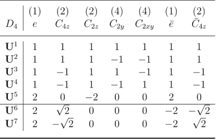
Table 2.1: The character table of the Dihedral Group D4. The horizontal line divides the

real irreps (U1 _to_U5_{) from the symplectic irreps (}_U6 _and _U7_).

(1) (2) (2) (4) (4) (1) (2) D4 e C4z C2z C2y C2xy e¯ C¯4z U1 ₁ ₁ ₁ ₁ ₁ ₁ ₁ U2 ₁ ₁ ₁ ₋₁ ₋₁ ₁ ₁ U3 1 ₋1 1 1 ₋1 1 ₋1 U4 ₁ ₋₁ ₁ ₋₁ ₁ ₁ ₋₁ U5 ₂ ₀ ₋₂ ₀ ₀ ₂ ₀ U6 ₂ √₂ ₀ ₀ ₀ ₋₂ ₋√₂ U7 ₂ ₋√₂ ₀ ₀ ₀ ₋₂ √₂

As an illustration, the character tables of the groups D4 and C4 are shown in Tables

2.1 and 2.2. Each row of a character table corresponds to a group irrep Uµ. The irrep in the first row is always the trivial irrep, where all group elements are identified on a one-dimensional space by the identity operator 1. The characters of this representation are trivially all equal to 1. The columns denote the conjugacy classes, e.g. e, C4z, etc.

and the number of elements in the conjugacy class, e.g. (1), (2), etc. The first column always shows the character of the identity element e, and is equal to the dimension n of the representation.

The symmetry group D4 plays an important role in QKD, as it is the symmetry group

of the signal states of the BB84 protocol. The group has 16 elements, divided into 7 conjugacy classes. Therefore, there are also 7 different irreps. The symmetry group C4 is

the symmetry group of the unbalanced phase-encoded BB84 protocol in Chapter 6. The group has 8 elements, 8 conjugacy classes, and 8 different irreps.

2.4.5 The complex conjugate irrep

Let U be an irrep of the group G with unitary operators Ug. The operators Ug can be

represented by n _×n matrices with complex matrix elements. We can construct a new irrep of the group G by taking the complex conjugate of the matrices with respect to a basis. The complex conjugate matrices then define the complex conjugate irrep U∗ [see

(35)

Table 2.2: The character table of the Cyclic GroupC4. The order of each conjugacy class is

one, and all irreps are one-dimensional. We define ω =e−iπ/4_{. The horizontal line divides}

the real irreps (U1 and U2) from the complex irreps (U3 to U8).

C4 e C4z C2z C4−z1 e¯ C¯4z C¯2z C¯4−z1 U1 1 1 1 1 1 1 1 1 U2 ₁ ₋₁ ₁ ₋₁ ₁ ₋₁ ₁ ₋₁ U3 1 ₋i ₋1 i 1 ₋i ₋1 i U4 ₁ _i ₋₁ ₋_i ₁ _i ₋₁ ₋_i U5 ₁ _ω ₋_i _ω7 ₋₁ _ω5 _i _ω3 U6 1 ω7 i ω ₋1 ω3 ₋i ω5 U7 ₁ _ω5 ₋_i _ω3 ₋₁ _ω _i _ω7 U8 ₁ _ω3 _i _ω5 ₋₁ _ω7 ₋_i _ω

for example Refs. [56, 17]]. Although complex conjugation depends on the choice of basis, the complex conjugate irreps defined in this way are all equivalent up to unitary rotations. There is a relationship between the irreps Uand U∗. If the irrep U is real, thenU∗ is necessarily also real, and therefore, U∗ ∼=U. If the vector space is complex, there are two cases: (i) The matrices of the irrep U have complex entries, but the characters χ(g) are real (symplectic irrep). Due to the uniqueness of the characters, it follows that U ∼= U∗. (ii) The matrices of the irrepUhave complex entries and the charactersχ(g) are complex (complex irrep). Then,U∗ is necessarily different from U.

In the character table of the Dihedral GroupD4 in Table2.1, the irrepsU1 throughU5

are real, andU6 and U7 are symplectic. For the Cyclic Group C4 in Table 2.2, the irreps U1 _and _U2 _{are real, and the rest are complex.}

(36)

2.4.6 Tensor products of irreps

Direct sum decomposition

The tensor product of two irrepsUµ_⊗_Uν _on_Hµ_⊗Hν _{is normally a reducible representation}

and can be decomposed into a direct sum of irrepsUω _{on Hilbert spaces} _Hω i: Hµ ⊗ Hν =M ω mω M i=1 Hω i. (2.65)

In this decomposition, the index i runs over 1, ..., mω, and the irrep Uω occurs mω times

in the decomposition.

Which irrepsUω _{appear in the direct sum decomposition? What are their multiplicities}

mω? Once the character table of a group G has been established there is a systematic

method to answer these questions based on character theory. The multiplicities mµ are

uniquely determined in the following theorem:

Theorem 6 The multiplicity mω of the irrep Uω in the direct sum decomposition (??) is

mω =hχµχν, χωi. (2.66)

The inner product between the characters is defined in Eq. (2.64), and χµ_χν _{is the character}

of the tensor product representation Uµ_⊗_Uν_.

In Chapter4, we are interested in the decomposition of tensor product representations of the form (Uµ)∗_⊗Uµ. The irreps Uµ describe transformations of the signal states of a QKD protocol. We calculate the decomposition for two examples.

Example 1 Let _HA and HB be two isomorphic qubit Hilbert spaces carrying the

two-dimensional irreps (U6₎∗ _and ₍_U6₎_{. We are interested in the decomposition of the tensor}

product

(U6)∗_⊗U6 :=UBB84 (2.67)

on the composite space_HA⊗ HB. SinceU6 is a symplectic irrep, it holds that(U6)∗ ∼=U6.

The character of the tensor product according to Eq. (2.63) is given by

e C4z C2z C2y C2xy e¯ C¯4z

(37)

The multiplicities mω for each irrep Uµ are given according to Eq. (2.66) by m1 =m2 =

m5 = 1 and m3 = m4 = m6 = m7 = 0. Therefore, the tensor product decomposes into

three irreps: two one-dimensional irreps U1 _and _U2_{, and one two-dimensional irrep} _U5

UBB84∼=U1 ⊕U5⊕U2. (2.69)

Example 2 We define the sum of two one-dimensional irrepsU1_⊕_U4 _{of the group}_C 4. Let

HAandHB be two isomorphic qubit Hilbert spaces carrying the representations(U1⊕U4)∗

and U1_⊕_U4_{. We are interested in the decomposition of the representation}

UUPE= (U1⊕U4)∗ ⊗(U1⊕U4) (2.70)

= ((U1)∗_⊗U1)_⊕((U1)∗_⊗U4)_⊕((U4)∗_⊗U1)_⊕((U4)∗_⊗U4) (2.71)

on _HA⊗ HB. From the uniqueness of the characters we determine that (U1)∗ ∼= U1 and

(U4₎∗ ∼

= U3_{. Furthermore, any product with the trivial irrep satisfies} _U1_⊗_Uµ ₌_Uµ_{. It}

remains to compute the direct sum decomposition of the product U3 _⊗_U4_{, which is easy}

because all irreps of C4 are one-dimensional. It follows that χ3χ4 = χ1, which uniquely

determines the decomposition

UUPE =U1⊕U4⊕U3⊕U1. (2.72) Clebsch-Gordan coefficients

LetUµ _and _Uν _{be two irreps of} _G _on_Hµ _and _Hν_{. We denote the bases of} _Hµ _and _Hν _by

{|iµi}i and{|jνi}j. The canonical basis onHµ⊗Hν is the tensor product basis{|iµ, jνi}i,j.

There exists a basis_{|φki}konHµ⊗Hν in which the direct sum decomposition ofUµ⊗Uν

is block diagonal in the matrix representation, namely

U_gµ_⊗U_gν _→      Uω1 g 0 0 0 0 U_gω2 0 0 0 0 0 0 . ..      . (2.73)

This new basis is related to the tensor product basis by the Clebsch-Gordan coefficients:

Definition 16 The coefficients _hiµ, jν|φki in the expansion |φki = P_i,jhiµ, jν|φki|iµ, jνi

(38)

The Clebsch-Gordan coefficients for tensor products of crystallographic groups representa-tions can be found in Ref. [17]

Continuing Example1, we define the canonical basis of the isomorphic spaces _HA and

HB by{|0i,|1i}. Then, the Clebsch-Gordan coefficients found in Ref [17] tell us that the

matrix representation of UBB84 ∼= (U6)∗ ⊗U6 is block diagonal in the Bell basis defined

in Eq. (2.10). Each irrep appearing in the direct sum decomposition of UBB84 lives on a

subspace spanned by the basis vectors of the Bell basis

U1 _{→ {|}Φ+_i} (2.74)

U5 _{→ {|}Φ−_i,_|Ψ+_i} (2.75)

U2 _{→ {|}Ψ−_i}. (2.76)

Note that U5 _{is a two-dimensional irrep, while} _U1 _and _U2 _{are both one-dimensional.}

2.4.7 Schur’s lemma

Schur’s lemma is a simple but powerful lemma.

Lemma 1 (Schur’s lemma). Let Uµ and Uν be irreducible representations of a group

G on Hilbert spaces _Hµ _and _Hν_{, and let} _A _{be a linear map from} _Hµ _{→ H}ν_{. If the linear}

map and the irreps commute,

A U_gµ =U_gν A, (2.77)

for all g _∈G, then A satisfies one of the two cases:

(i) if Uµ ∼= Uν, A = c 1n, where c ∈ C is a scalar and 1n is the identity operator

mapping _Hµ_{→ H}ν. (ii) ifUµ

Uν, then A is equal to zero.

We continue Example 1. Suppose a density operator ρA ∈ D(HA) commutes with all

group elements ofU6_:

(39)

It follows from (i) in Schur’s lemma that ρA is proportional to the identity 12. In the

matrix formulation with the proper normalization trρA = 1 this amounts to

ρA= 1 212 = 1 2 1 0 0 1 . (2.79)

Let ρAB be a composite density operator on D(HAB). Suppose ρAB commutes with the

representationUBB84= (U6)∗⊗U6 of the groupD4 onHAB:

[ρAB, Ug6⊗U

6

g] = 0, ∀g ∈G. (2.80)

Since we know that the direct sum decomposition of UBB84 is block-diagonal in the Bell

basis, let us parametrizeρAB in the Bell basis by

ρAB =     ρ11 ρ12 ρ13 ρ14 ρ∗₁₂ ρ22 ρ23 ρ24 ρ∗₁₃ ρ∗₂₃ ρ33 ρ34 ρ∗₁₄ ρ∗₂₄ ρ∗₃₄ ρ44     . (2.81)

Then, the diagonal blocks ofρAB satisfy the following commutation relations

ρ11Ug1 =U 1 g ρ11, (2.82) ρ22 ρ23 ρ∗₂₃ ρ33 U_g5 =U_g5 ρ22 ρ23 ρ∗₂₃ ρ33 , (2.83) ρ44Ug2 =U 2 g ρ44. (2.84)

The commutation relation of the off-diagonal blocks of ρAB is given by

ρ12 ρ13 U_g5 =U_g1 ρ12 ρ13 , (2.85) ρ14Ug2 =U 1 g ρ14, (2.86) ρ24 ρ34 U_g2 =U_g5 ρ24 ρ34 . (2.87)

We apply Schur’s lemma to each of the blocks individually. All diagonal blocks satisfy (i) in Schur’s lemma, while all off-diagonal blocks satisfy (ii). Hence,

ρ11=a11, (2.88) ρ22 ρ23 ρ32 ρ33 =b12, (2.89) ρ44=c11, (2.90)

(40)

wherea, b and care constants. All other entries are zero. Thus, ρAB =     a 0 0 0 0 b 0 0 0 0 b 0 0 0 0 c     (2.91)

(41)

Chapter 3 Quantum key distribution

background

This chapter is a background chapter about quantum key distribution. References can be found in [86,39, 77].

3.1 QKD protocols

The objective of QKD is to establish a secret key between two legitimate parties, Alice and Bob. The secret key can be used later in classical cryptographic applications, for example to facilitate secure communication.

A secret key is a string k of independent and uniformly distributed random variables, that is known to Alice and Bob, but unknown to any eavesdropper, Eve. In order to generate a secret key, Alice and Bob follow a protocol with well-defined steps. Typically, the protocol has a quantum phase and the classical phase. In the quantum phase, Alice and Bob exchange quantum signals over a quantum channel. In the classical phase, they communicate over an authenticated classical channel and extract a secret key using classical communication protocols. During the whole process, the goal of the eavesdropper is to learn about the key by launching anattack on the protocol.

First, we describe the steps of a protocol in the prepare-and-measure scheme.

(42)

1. Preparation. Let S = _{|ϕxi, x = 1,2, ...,|S|} be a set of |S| quantum states |ϕxi

defined on a d-dimensional Hilbert space _HS. Alice chooses n states (signal states)

with probability p(x) from the set S in her laboratory. The quantum states encode the random variables of the key. Alice keeps a record of the chosen sequence of quantum states before sending them over a quantum channel to Bob.

2. Measurement. Bob measures the quantum states in his laboratory by means of a POVM MB = {FBy}y. He records the measurement outcomes, which results in

cor-related data (raw data) according to the conditional probability distribution p(y_|x), shared between Alice and Bob.

Classical phase:

1. Parameter estimation. Alice and Bob publicly announce a small amount of their data to determine the statistics of the remaining data. If the statistics indicate that the remaining data is suitable to generate a key, the protocol continues, otherwise it aborts.

2. Postprocessing. Alice and Bob can process their data to their advantage. For exam-ple, they can discard data that they identify to be unsuitable for the key. Then they agree how to map their data to the actual key values.

3. Error correction. If the key strings are not perfectly correlated Alice and Bob perform error correction (sometimes called reconciliation), to generate a pair of perfectly correlated, but shorter strings. A typical choice for the error correction is one-way error correction, in which the data of one party is set as a reference key. The party with the reference key sends error correction information to the other party, who then must correct her or his noisy data to match the reference key. We speak of

direct/reverse reconciliation, if Alice’s/Bob’s data serves as the reference key. If the error correction is successful, Alice and Bob share two identical strings. There is also the possibility that the error correction fails, and the protocol aborts.

4. Privacy amplification. In the last step, Alice and Bob eliminate Eve’s information about their strings through privacy amplificaion. They obtain two shorter strings

kA=kB ≡ k of length ` ≤n on which Eve has no information. For this to succeed,

Alice and Bob need to be able to upper bound the amount of information Eve knows about the correlated data. If the privacy amplification is successful, Alice and Bob generate a secret key, otherwise, the protocol aborts.

(43)

3.1.1 Source-replacement scheme

The preparation step of the quantum phase is equivalently described in thesource-replacement scheme, which is convenient scheme to analyze the security of a protocol. The source-replacement scheme is a thought setup, in which Alice creates a hypothetical bipartite entangled state (source state)

|Φ_i=X

x

p

p(x)_|x_iX|ϕxiS (3.1)

in her laboratory, keeps the first half for herself and sends the other half to Bob. The states |x_i form an orthonormal basis _X = _{|x_i, x= 0, ...,_|S_{| −}1_} of an _|S_|-dimensional Hilbert space _HX. In order to prepare the state |ϕxi on Bob’s side, Alice performs a projective

measurement in the basis_X, which triggers the source state to collapse onto the conditional state _|ϕxi with probabilityp(x).

If the signal states are linearly dependent, the source state assumes a more compact form. We define a d-dimensional subsystem A of the system X, and express the source state on the “compact” Hilbert space_HA⊗ HS

|Φ_iAS = d−1 X i=0 √_κ i|¯iiA|iiS. (3.2)

In this expression, the basis _B = _{|i_iS;i = 0, ..., d − 1} is the Schmidt basis, and the

coefficients √κi are the Schmidt coefficients. They are the eigenbasis and the square

roots of the eigenvalues of the reduced operator φS = trX{|ΦiXShΦ|}. The Schmidt basis

A = _{|¯i_iA;i = 0, ..., d−1} of the system A can be explicitly given by the orthonormal

vectors _|¯i_i =P

x

p

p(x)α(_ix)_|x_i/√κi, where α

(x)

i =hi|ϕxi are the coefficients of the signal

states in the Schmidt basis_B. In the following, we omit the bar in _|¯i_i.

Alice’s projective measurement in the basis_X on_HX is equal to a measurementMA=

{Fx

A}x with respect to rank-one POVM elements FAx on the smaller space HA given by

F_Ax =p(x)√ρA

−1

|ϕ∗_x_ihϕ∗_x_|√ρA

−1

. (3.3)

Here we define the density matrix of Alice’s reduced state as

ρA= trS{|ΦiAShΦ|}, (3.4)

and the states

|ϕ∗_x_i=X i hϕx|ii |ii= X i (α(_ix))∗ _|i_i, (3.5)

Security proof methods for quantum key distribution protocols