Physics and Astronomy Publications Physics and Astronomy 10-13-2020
Efficient Step-Merged Quantum Imaginary Time Evolution
Efficient Step-Merged Quantum Imaginary Time Evolution
Algorithm for Quantum Chemistry
Algorithm for Quantum Chemistry
Niladri GomesAmes Laboratory, [email protected]
Feng Zhang
Ames Laboratory, [email protected]
Noah F. Berthusen
Iowa State University and Ames Laboratory, [email protected]
Cai-Zhuang Wang
Iowa State University and Ames Laboratory, [email protected]
Kai-Ming Ho
Iowa State University and Ames Laboratory, [email protected]
See next page for additional authors
Follow this and additional works at: https://lib.dr.iastate.edu/physastro_pubs
Part of the Other Chemistry Commons, Other Computer Sciences Commons, and the Other Electrical and Computer Engineering Commons
The complete bibliographic information for this item can be found at https://lib.dr.iastate.edu/physastro_pubs/707. For information on how to cite this item, please visit http://lib.dr.iastate.edu/howtocite.html.
This Article is brought to you for free and open access by the Physics and Astronomy at Iowa State University Digital Repository. It has been accepted for inclusion in Physics and Astronomy Publications by an authorized administrator of Iowa State University Digital Repository. For more information, please contact [email protected].
Efficient Step-Merged Quantum Imaginary Time Evolution Algorithm for Quantum
Efficient Step-Merged Quantum Imaginary Time Evolution Algorithm for Quantum
Chemistry
Chemistry
Abstract Abstract
We develop a resource-efficient step-merged quantum imaginary time evolution approach (smQITE) to solve for the ground state of a Hamiltonian on quantum computers. This heuristic method features a fixed shallow quantum circuit depth along the state evolution path. We use this algorithm to determine the binding energy curves of a set of molecules, including H2, H4, H6, LiH, HF, H2O, and BeH2, and find highly accurate results. The required quantum resources of smQITE calculations can be further reduced by adopting the circuit form of the variational quantum eigensolver (VQE) technique, such as the unitary coupled cluster ansatz. We demonstrate that smQITE achieves a similar computational accuracy as VQE at the same fixed-circuit ansatz, without requiring a generally complicated high-dimensional nonconvex optimization. Finally, smQITE calculations are carried out on Rigetti quantum processing units,
demonstrating that the approach is readily applicable on current noisy intermediate-scale quantum devices.
Keywords Keywords
Chemical calculations, Mathematical methods, Circuits, Hamiltonians, Molecules
Disciplines Disciplines
Other Chemistry | Other Computer Sciences | Other Electrical and Computer Engineering
Comments Comments
This document is the unedited Author’s version of a Submitted Work that was subsequently accepted for publication in Journal of Chemical Theory and Computation, copyright © American Chemical Society after peer review. To access the final edited and published work see DOI: 10.1021/acs.jctc.0c00666. Posted with permission.
Authors Authors
Niladri Gomes, Feng Zhang, Noah F. Berthusen, Cai-Zhuang Wang, Kai-Ming Ho, Peter P. Orth, and Yongxin Yao
Efficient step-merged quantum imaginary time
evolution algorithm for quantum chemistry
Niladri Gomes,
†Feng Zhang,
†Noah F. Berthusen,
†,‡Cai-Zhuang Wang,
†,PKai-Ming Ho,
†,PPeter P. Orth,
†,Pand Yongxin Yao
∗,†,P†Ames Laboratory, U.S. Department of Energy, Ames, Iowa 50011, USA
‡Department of Electrical and Computer Engineering, Iowa State University, Ames, Iowa 50011, USA.
PDepartment of Physics and Astronomy, Iowa State University, Ames, Iowa 50011, USA E-mail: [email protected]
Abstract
We develop a resource efficient step-merged quantum imaginary time evolution approach (smQITE) to solve for the ground state of a Hamiltonian on quantum computers. This heuristic method features a fixed shallow quan-tum circuit depth along the state evolution path. We use this algorithm to determine binding energy curves of a set of molecules, including H2, H4, H6, LiH, HF, H2O and BeH2, and find
highly accurate results. The required quantum resources of smQITE calculations can be further reduced by adopting the circuit form of the vari-ational quantum eigensolver (VQE) technique, such as the unitary coupled cluster ansatz. We demonstrate that smQITE achieves a similar computational accuracy as VQE at the same fixed-circuit ansatz, without requiring a gener-ally complicated high-dimensional non-convex optimization. Finally, smQITE calculations are carried out on Rigetti quantum processing units (QPUs), demonstrating that the approach is readily applicable on current noisy intermediate-scale quantum (NISQ) devices.
1
Introduction
One of the most promising near-term applica-tions of quantum computing is to solve the
elec-tronic structure of molecules and condensed mat-ter systems.1–7 This is because the number of
binary bits required to store a general many-body state of a fermionic Hamiltonian grows exponentially with the dimension of the single-particle basis in classical computers, while quan-tum computers offer a natural representation of many-body states using qubits whose required number only scales linearly with the size of the single-particle basis. A many-body wave func-tion can thus be efficiently stored in memory using qubits. The pioneering proposal of quan-tum phase estimation algorithm (PEA) needs O(1/) controlled-U operators and O(log(1/)) ancillary qubits to reach an accuracy, whereU
is the time-evolution operator of a given system Hamiltonian.8,9 This represents a very stringent
requirement for the quantum resources in terms of number of qubits, gate fidelity and coherence time, which is beyond the current or near-term NISQ computing technology. While the number of ancillary qubits can be significantly reduced by adopting the recursive PEA,2 the general
condition of deep quantum circuits in the PEA and the adiabatic state preparation (ASP) re-mains prohibitive for practical calculations on NISQ devices.
A large class of algorithms adapted to NISQ hardware have been developed in recent years, to exploit the new technology in Hamiltonian simulations, or a wider set of optimization
prob-lems.5,10–20The variational quantum eigensolver
(VQE) represents a most promising approach to address open quantum chemistry problems us-ing NISQ technologies.11–14,16 Within VQE, the
state wavefunction is parameterized by a varia-tional ansatz. The cost function, which is usu-ally the expectation value of the system Hamilto-nian with respect to the variational ansatz, can be efficiently calculated on NISQ devices with relatively shallow circuits. The variational pa-rameters are adjusted to extremize the cost func-tion using classical computers. The effectiveness of VQE is determined by the variational wave-function form and the high-dimensional clas-sical optimization. The unitary coupled clus-ter ansatz with single and double excitations (UCCSD) represents a commonly used
varia-tional form, motivated by the success of the CCSD method in classical quantum chemistry calculations for systems free of multi-reference characters.21–23 Many efforts have been devoted
to improve the variational ansatz regarding the computational accuracy and variational circuit complexity.5,16–20,24For examples, the
hardware-efficient ansatz prepares the variational state by a sequence of native two-qubit entangling gates alternating with single qubit Euler rotations to an initial state such as Hartree-Fock (HF) state.16 The k-UpCCGSD ansatz is composed
of k products of generalized unitary paired dou-ble excitations and a complete set of generalized single excitations, which can be systematically improved toward exact answers.18The quantum
approximate optimization algorithm (QAOA) provides an alternative way to construct a vari-ational ansatz in the form of applying the sys-tem Hamiltonian and mixing Hamiltonian to a reference state.10 The variational wavefunction
form has also been proposed to be dynamically optimized, which provides a compact system-dependent ansatz with systematically improv-able accuracies.17,19,20
While the variational wavefunction form in VQE can be optimized to some extent, the num-ber of variational parameters is deemed to grow with the system size under study. The cost func-tion of VQE is generally non-convex in the high-dimensional parameter space, which renders the classical optimization problem susceptible to
lo-cal minima and very challenging.13 Recently, a
quantum imaginary time evolution algorithm (QITE) has been proposed as an alternative
ap-proach to determine eigenstates of an Hamilto-nian on quantum computers without the compli-cation of high-dimensional optimization.25 The idea originates from the classical imaginary time evolution algorithm, which is a sophisticated way to obtain Hamiltonian eigenstates using classical computers.26,27 Within the QITE algo-rithm, the non-unitary imaginary time evolution operator is replaced by a unitary operator which preserves the induced variation in the quantum state. The unitary operator is uniquely deter-mined by solving a system of linear equations and can be conveniently applied on quantum computers. The QITE method has been demon-strated by solving a set of finite spin models on quantum simulators, including a two-site Ising model and H2 dimer on real quantum
de-vices.25,28
As the current and near term NISQ hardware suffers short coherence time, gate infidelity, and other noises, the direct application of QITE on real devices is limited by the rather deep quantum circuits, in particular for systems with long-range correlations. The circuit depth grows linearly with the QITE steps, similar to the cir-cuit to study the quantum dynamics following Trotter decomposition for the time-evolution op-erator.29,30 In contrast, the VQE calculations with an ansatz such as UCCSD features a varia-tional circuit of fixed depth. In this paper, we develop a resource-efficient “step-merged” QITE (smQITE) algorithm, which performs
approxi-mate QITE calculations at fixed quantum circuit depth. The smQITE method builds on the nu-merical observations that the accumulated uni-tary operators in the QITE calculation can often be effectively combined. We will first present the smQITE formalism, followed by demonstra-tions that the smQITE method can produce high-quality results beyond chemical accuracy on a set of molecules. We demonstrate that the circuit depth of smQITE calculations can be further reduced significantly by adopting com-pact wavefunction representations, such as the UCCSD variational form among others, which ef-fectively reduce the circuit depth down to that of
UCCSD-VQE. It is shown that smQITE method can reach the accuracy of VQE with the same UCCSD ansatz, in much fewer steps without resorting to high-dimensional optimizations. Fi-nally, we demonstrate the smQITE calculations for H2 dimer on a real quantum device, with
a binding energy curve in reasonable accuracy. We argue that, supported by numerical evidence, a combination of smQITE with VQE offers a way to address the highly complicated optimiza-tion problem of VQE when simulating large molecules.
2
Step-merged QITE
algo-rithm
To be self-contained, we first review the quan-tum imaginary time evolution algorithm pro-posed by Motta et al,25 and point out the
limi-tations for practical implemenlimi-tations on NISQ devices. The presentation of the step-merged QITE (smQITE) formalism then follows, which aims to dramatically reduce the circuit depth of QITE calculations on quantum computers, hence is better adapted for the current and near-term quantum devices.
2.1
QITE algorithm
Consider an Nq-qubit system with Hamiltonian
ˆ
H = PM−1
m=0 hˆ[m], which includes a sum of M
weighted Pauli terms. The Pauli term ˆh[m] is a general product of Pauli operators. The qubit Hamiltonian can naturally describe spin-12 mod-els, or fermionic systems by mapping fermionic operators to qubit operators.31,32 Starting from an initial state |Ψ0i, the imaginary time
evolu-tion leads the system to the lowest eigenstate |Ψfi which has finite overlap with |Ψ0i in the
long time limit,
|Ψfi = lim β→∞e
−βHˆ|
Ψ0i. (1)
The imaginary time evolution can be carried
out through Trotter decomposition33
e−βHˆ = (e−∆τhˆ[0]e−∆τˆh[1]· · ·)N
+O(∆τ), (2) with the Trotter step size ∆τ = Nβ. Literally, the above evolution operator e−βHˆ consists of
M ×N steps, yielding an error of leading order proportional to ∆τ. For the convenience of discussions later, we label the Trotter step by (n, m) ≡ nM +m, with 0 ≤ n < N and 0 ≤
m < M. The associated intermediate state is
labelled as Ψ(n,m). After one additional Trotter
evolution step, we have
Ψ(n,m)+1 =c− 1 2 (n,m)e −∆τˆh[m] Ψ(n,m) , (3)
The wavefunction norm is given by
c(n,m) = hΨ(n,m)|e−2∆τ ˆ h[m]|Ψ (n,m)i = 1−2∆τhΨ(n,m)|hˆ[m]|Ψ(n,m)i +O(∆τ2), (4) where to leading order in ∆τ the deviation of the norm from unity is determined by the expecta-tion value of the Hamiltonian in the intermediate state.
The main idea of QITE algorithm is to replace the non-unitary imaginary time Trotter evolu-tion operator in Eq. (3) by a unitary operator which transforms Ψ(n,m) to a state closest to
Ψ(n,m)+1, Ψ(n,m)+1 ≈e−i∆τAˆ(n,m)Ψ(n,m) . (5)
Here, ˆA(n,m) is a Hermitian operator that can be expanded in a complete Pauli basis set of a domain ofD qubits around the support of ˆh[m]:
ˆ
A(n,m) ≡X
I
a(In,m)σˆI. (6)
Here, I = i0i1...iD is a composite index
run-ning through all the D qubits. The domain D
includes at least all sites m, where ˆh[m] acts non-trivially. Generally, the domain size D can be larger than the support of a qubit opera-tor due to correlation effects.25 The Pauli term ˆ
ˆ
σi ∈ {I, X, Y, Z} is a Pauli operator associated
with the ith qubit. Without loss of generality,
a(n,m) is a set of real parameters of dimension 4D corresponding to rotation angles in the qubit
Hilbert space.
In order to determine the operator ˆA(n,m), we define the change of the state wavefunction after a Trotter imaginary time evolution step as
∆ (n,m) 0 E = Ψ(n,m)+1 − Ψ(n,m) ∆τ (7) ≈ c− 1 2 (n,m)−1 ∆τ −c −1 2 (n,m)ˆh[m] Ψ(n,m) ,
where the Trotter exponential operator in Eq.3 is expanded to the first order of ∆τ. Similarly, for the unitary evolution we define the variation of the state as.
∆ (n,m) 1 E = e −i∆τAˆ(n,m) Ψ(n.m) −Ψ(n,m) ∆τ ≈ −iAˆ(n,m)Ψ(n,m) . (8)
The objective function to be minimized is de-fined as f[a] = h∆(0n,m)−∆1(n,m)|∆0(n,m)−∆(1n,m)i (9) = f0+ X I bIa (n,m) I + X IJ a(In,m)SIJa (n,m) J with f0 =h∆ (n,m) 0 |∆ (n,m) 0 i, (10) bI = −ih∆ (n,m) 0 |σˆI|Ψ(n,m)i+c.c, (11) ≈ ic− 1 2 (n,m)hΨ(n,m)|ˆh[m]ˆσI|Ψ(n,m)i+c.c., and SIJ =hΨ(n,m)|σˆ † IˆσJ|Ψ(n,m)i. (12)
The minimization of the function f[a] with re-spect to a(n,m) leads to a system of linear
equa-tions
S +STa(n,m) =−b, (13) which is solved to determine the optimal expan-sion coefficients a(n,m) for the operator ˆA(n,m). Since f0 does not enter the above linear
equa-tion, no explicit evaluation is needed. Quantum computers are employed to facilitate the setup
of the linear equation (13) by determining theS -matrix and b-vector. As the quantum computa-tion only involves direct measurements of Pauli terms with respect to the state wavefunction, it is straightforwardly implemented on quan-tum devices. The number of linear equations in Eq. (13) is 4D, which scales exponentially
with the number of qubits D in the relevant qubit domain. With increasing system size, this rapidly becomes the bottleneck of the algorithm. We will discuss alternative ways to lift this con-straint in section 3.3.
2.2
Step-merged QITE
A key factor in determining the required quan-tum resources of the QITE approach is the preparation of state Ψ(n,m) at Trotter step
(n, m), which will be repeated for all the mea-surements. The state Ψ(n,m) is constructed as
Ψ(n,m) = m Y µ0=0 e−i∆τAˆ(n,µ 0) × n−1 Y ν=0 M−1 Y µ=0 e−i∆τAˆ(ν,µ)|Ψ0i,(14)
where the exponential operators are ordered ac-cording to the Trotter evolution path, as also illustrated in Fig. 1. Clearly, the depth of the state preparation circuit grows linearly with the Trotter steps, which limits the system size and maximal Trotter steps that the QITE algorithm can perform in NISQ devices. In contrast, the variational quantum algorithms, such as varia-tional quantum eigensolver with unitary coupled cluster ansatz,13,34 have an advantage of a varia-tional quantum circuit at fixed depth. Although some approximate ways have been discussed in references,25,28,35 the linear growth of the quan-tum circuit depth with increasing Trotter steps has not been addressed.
Here, we propose a step-merged QITE (smQITE) approach to control the circuit depth at an effective single (or few) Trotter step level. The key idea is to combine Trotter evolution unitaries along the state evolution path, which act on a common set of qubits. The algorithm is schematically depicted in Fig. 1. While this
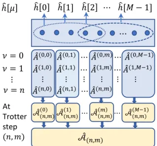
heuristic approach does not become exact in the limit N → ∞, we show below that it leads to results for ground state energies that are comparable to VQE. This is remarkable as, unlike VQE, the smQITE approach does not require performing a difficult optimization in a high-dimensional feature space. We further discuss a systematic way to improve the accu-racy of smQITE at the cost of using deeper circuits. Finally, the smQITE method can also be combined with VQE, as it yields an efficient ansatz for the ground state that can be further optimized variationally. ℎ 0 ℎ[1] ℎ 2 ⋯ ℎ[𝑀 − 1] ⋯ ℎ 𝜇 መ 𝐴(0,0) 𝐴መ(0,1) ⋯ መ𝐴(0,𝑚)⋯ መ𝐴(0,𝑀−1) 𝜈 = 0 መ 𝐴(1,0) 𝐴መ(1,1) ⋯ መ𝐴(1,𝑚)⋯ መ𝐴(1,𝑀−1) 𝜈 = 1 ⋮ ⋮ ⋮ ⋮ ⋮ ⋮ At Trotter step (𝑛, 𝑚) መ 𝐴(𝑛,0) 𝐴መ(𝑛,1) ⋯ መ𝐴(𝑛,𝑚) መ 𝒜(𝑛,𝑚)(0) 𝒜መ(𝑛,𝑚)(1) ⋯ መ𝒜𝑛,𝑚𝑚 ⋯ 𝒜መ(𝑛,𝑚)(𝑀−1) መ 𝒜(𝑛,𝑚) ⋮ 𝜈 = 𝑛
Figure 1: Schematic illustration of com-bining Trotter unitaries in smQITE algo-rithm. At Trotter step (n, m) with imaginary time evolution operator e−∆τˆh[m], a new unitary
operatore−i∆τAˆ(n,m) is appended to the quantum circuit. The operator ˆA(n,m) is defined in a qubit domainDm around the support of ˆh[m]. A set of
Pauli terms in the qubit Hamiltonian can share a common qubit domain, as indicated by the dotted ellipse. As the accumulated operators {Aˆ(ν,µ)} at Trotter step (n, m) share the same qubit domain if they have the same column index
µ, they can be combined to ˆA((µn,m) ) =P
νA
(ν,µ).
By defining a union of the Pauli basis set in all qubit domains D= D0 ∪. . .∪DM, the
op-erators {Aˆ((µn,m) )} can be further combined to a single operator ˆA(n,m) =PM
−1
µ=0 Aˆ (µ) (n,m).
More specifically, by commuting terms with a
common index µ next to each other in Eq. (14), we can rewrite the state evolution in this equa-tion as Ψ(n,m) =e−i∆τ PM−1 µ=0 Aˆ (µ) (n,m)|Ψ 0i+O(∆τ2). (15) Here, we have defined ˆA((µn,m) )=Pn
ν=0A(ν,µ) for µ ≤ m. For µ > m, the summation stops at
ν =n−1. This expression combines the oper-ators ˆA(ν,µ) with a common index µthat share
the same Pauli basis in the qubit domain Dµ
around the support of h[µ]. By commuting the exponential terms to bring terms with a com-mon µ next to each other, we have generated a number of terms that are all of the order of ∆τ2. We discuss the issue of the Trotter error
in more detail below.
Further grouping is possible if different qubit domains Dµ of different ˆh[µ] overlap and some
ˆ
A(µ)-operators can be further combined.
With-out loss of generality, we define an extended Pauli basis set{σI} as the union of all the Pauli
basis sets in the different qubit domains Dµ of
the Hamiltonian terms {ˆh[µ]}. This allows us to maximally combine the operators ˆA(n,m) ≡
PM−1
µ=0 Aˆ (µ)
(n,m) and represent it in the extended
Pauli basis set, as illustrated in Fig. 1. The smQITE wavefunction at Trotter step (n, m) is then given by Ψ(n,m) =e−i∆τAˆ(n,m)|Ψ 0i , (16)
which corresponds to a single effective Trotter step. Note that in the original QITE paper,25
ˆ
h[m] is defined according to operational local-ity and can be a sum of Pauli terms sharing a common qubit domain. Therefore, an effective combination of ˆA(ν,µ) over indexµat a common
qubit domain has been performed, albeit at each individual Trotter step ν.
In the case ofab initiomolecular Hamiltonians where long-range one-body and two-body opera-tors are present, it is often the case that the set of {hˆ[µ]} Hamiltonian terms share a common domain of qubits, that often spans the full sys-tem. It is thus natural to consider the evolution under the full Hˆˆ:
Ψ(n+1) =c− 1 2 (n)e −∆τHˆ Ψ(n) , (17)
rather than Eq. (3). Note that we do not in-troduce the domain index µas there is only a single domain spanning the full system. The state evolution Eq. (15) thus reads as
Ψ(n) =e−i∆τAˆ(n)|Ψ 0i, (18) with ˆA(n) = Pn −1 ν=0Aˆ (ν) = P I Pn−1 ν=0a (ν) I ˆ σI,
where we have combined Trotter unitaries with different step index ν. The step of combined Trotter evolution of the state wavefunction across the whole set of {ˆh[µ]}does not change the quantum circuit depth. However, it poten-tially saves time for systems with largely over-lapping qubit domains{Dµ}, such as molecules,
due to the prevalence of nonlocal one-body and two-body operators. Furthermore, it introduce a new perspective that a compact representation of the ˆAnoperator can be obtained through
vari-ational wavefunction forms of VQE, which will be detailed in section 3.3. It has been discussed recently that the Pauli operator ordering in the Trotterized circuits of the VQE-UCCSD ap-proach can introduce significant errors in energy evaluations beyond chemical accuracy.36 As a Trotterized form is also adopted in the smQITE method, similar operator ordering effects could exist. Nevertheless, we will demonstrate that decent numerical results from smQITE calcula-tions can already be obtained without exploiting optimum Pauli operator orderings. For the pur-pose of reproducibility of numerical results, all our calculations, including explicit ordered list of Pauli operators, are publicly accessible in the online repository.37
As the number of Trotter steps N increases, the smQITE approach maintains a favorable fixed circuit depth. This is in stark contrast to the linear growth of the depth with N found in QITE.25 But the gain in quantum resource effi-ciency is obtained at a price. In the worst case scenario where none of the operators {Aˆ(ν,µ)}
commute with each other and all leading Trot-ter errors are of the same sign and add up, the above step merging procedure introduces a con-stant error. The smQITE approach thus loses the mathematical rigor of QITE and does not become exact in the limit of small Trotter step
size ∆τ =β/N −−−→N→∞ 0. The smQITE method should thus be regarded as a heuristic approach that can still work well in the average case, as we demonstrate for a number of examples below. Even in this worst case scenario where the Trot-ter error is uncontrolled, the energy obtained from the smQITE ansatz is still a variational upper bound, and the smQITE wavefunction
Ψ(n,m)
in Eq. (16) can be used as a starting point for further variational optimization us-ing VQE. It is worth notus-ing that the operator
ˆ
A(n,m) in Eq. (6) is first determined
variation-ally at each smQITE step, and subsequently merged into the preceding unitary operators. In other words, the QITE procedure is followed initially, but in order to avoid a further growth of the circuit depth the preparation of state
Ψ(n,m)
is approximately achieved by using the step-merged unitary in Eq. (16). Therefore, the effective single-step smQITE ansatz is generally different form the a QITE ansatz with a sin-gle Trotter step. In fact, because the smQITE approach coincides with QITE at the first Trot-ter step where no combination of unitaries has been performed, smQITE can always achieve the single-step QITE result as an upper bound. The error in smQITE calculations should be equal or smaller than that by effectively reducing the Trotter decomposition in Eq. (2) from orderN
to order 1, which will also be demonstrated nu-merically in section 3.2.
Finally, let us describe a way to detect the Trotter errors induced by the step merging pro-cess and a way to iteratively reduce it. One way to estimate this error is to compare the energy of the state obtained from merging all Trotter steps ν into a single effective step,
ˆ
A((µn,m) ) =Pn
ν=0A
(ν,µ), versus merging them into
two effective steps, Aˆ((ν,µn,m)) = Pn2(ν+1)
ν0=n
2ν
A(ν0,µ)
with ν = 0,1. If the energy decreases when using more effective Trotter steps, this process can be repeated until convergence. Obviously, this process approaches the original QITE limit if we increase the range of the indexνand hence requires increasingly deep circuits to prepare the wavefunctionΨ(n,m)
3
Application of step-merged
QITE to quantum
chem-istry
In this section, we show that highly accurate results beyond chemical accuracy can be ob-tained for the smQITE calculations for a set of molecules. In particular, we prove numeri-cally that the high accuracy of smQITE method cannot be obtained by instead using a single Trotter step calculation, even when using an op-timum step size ∆τ. We further propose a way to effectively adopt the variational wavefunction form of VQE into smQITE. For a number of molecules, we show that smQITE yields results of similar accuracy as VQE with the same fixed variational ansatz, yet with much fewer steps and shallower circuits. Finally, we report results of smQITE calculations performed on Rigetti QPUs.
3.1
Implementation of smQITE
for quantum chemistry
Consider an ab initio nonrelativistic molecular electron Hamiltonian ˆ H = X pq X σ hpqˆc†pσˆcqσ + 1 2 X pqrs X σσ0 hpqrsˆc†pσcˆ † rσ0cˆsσ0cˆqσ, (19)
with the one-electron core part of the Hamilto-nian given by
hpq =
Z
drφ∗p(r)(T +Vion)φq(r), (20)
and the two-electron Coulomb integral
hpqrs = Z dr Z dr0φ∗p(r)φ∗r(r0)Veeφs(r0)φq(r). (21)
Here p, q, r, s are composite indices for atom
and orbital, and σ is spin index with values of α for spin-up and β for spin-down. T is the kinetic energy operator, Vion is the ionic
potential operator and Vee the Coulomb
inter-action operator. {φ(r)}is a set of basis orbital
functions, which are obtained from the stan-dard STO-3G minimal basis set. In the follow-ing smQITE calculations of molecules, a quan-tum chemistry package PySCF is first used to get the restricted Hartree-Fock(HF) solution.38
The molecular Hamiltonian (Eq. 19) is then transformed to the molecular orbital represen-tation for the convenience of preparation of the initial HF state in quantum computer. The qubit representation of the Hamiltonian is ob-tained by parity transformation, with two qubits reduced by exploiting the conservation of to-tal number of electrons and Z-component of the total spin operator, e.g., the Z2
symme-try. The smQITE code is implemented using modules from Qiskit39 and Forest,40,41 and is available as a module in the open-source package PyGQCE.42 The smQITE method is a general Hamiltonian eigensolver, with potential appli-cations beyond quantum chemistry problems, such as the impurity models.7
3.2
smQITE calculations using a
complete Pauli basis set
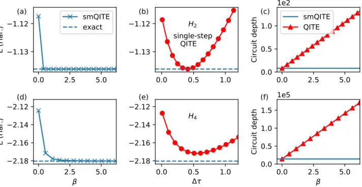
Figure 2 shows the evolution of the Hamiltonian expectation valueE as a function ofβ = n×∆τ
for H2 dimer and H4 chain in panel (a) and (d),
which quickly converges to the exact result from the initial value of the HF solution. In the mid-dle panels (b) and (e), we plot the energy E
after a single QITE step upon the initial HF wavefunction with varying the Trotter step size ∆τ, which shows a polynomial behavior with a unique minimum Emin(1) at an optimal step size ∆τopt. Accidentally,E
(1)
min coincides with the
ex-act energy for H2, which is due to the simple
structure of the Hamiltonian. Generally, Emin(1)
will be higher than the exact result. For the case of H4, the energy is overestimated by 5
kcal/mol, which is beyond the chemical
accu-racy of 1 kcal/mol.43 For comparison, ∆τ
opt is
used as the fixed step size ∆τ for the smQITE calculations. Fig. 2(b) clearly shows that the smQITE calculation of H4 can reach a much
higher accuracy ( 10−4kcal/mol) after a few
steps. The calculations are performed on a wave-function simulator as implemented in Forest,40,41
0.0
2.5
5.0
1.13
1.12
E (Har.)
(a)
smQITE
exact
0.0
0.5
1.0
1.13
1.12
(b)
H
2single-step
QITE
0.0
2.5
5.0
0.0
0.5
1.0
Circuit depth
1e2
(c)
smQITE
QITE
0.0
2.5
5.0
2.18
2.16
2.14
2.12
E (Har.)
(d)
0.0
0.5
1.0
2.18
2.16
2.14
2.12
(e)
H
40.0
2.5
5.0
0.0
0.5
1.0
1.5
Circuit depth
1e5
(f)
Figure 2: Energy convergence and fixed circuit depth of the smQITE method. Upper panels show the energy evolution as a function of merged QITE steps (a), the energy as a function of single QITE step size (b), and the quantum circuit depth of QITE and smQITE calculations (c) for H2 dimer at bond length 0.7˚A, together with the results for H4 chain at bond length 0.9˚A in
lower panels. Note that the circuit depth at order of 105 is far beyond the capability of the current
NISQ devices.
which is equivalent to perfect measurements on fault-tolerant quantum computers. We estimate the quantum circuit depth by counting the num-ber of two-qubit controlled-NOT (CNOT) gates in the algorithms, which are shown in Fig. 2(c) and (f) for calculations of H2 and H4,
respec-tively. As expected, the smQITE circuit has a fixed depth at 8 for H2and 14208 for H4. In
con-trast, the QITE circuit grows linearly in depth as the QITE step proceeds.
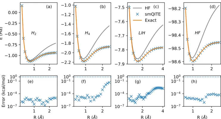
We further apply the smQITE method to a set of molecules to map out the full binding and dissociation energy curves, which give a more complete assessment of the computational accu-racy. The smQITE results are reported with the exact curves in Fig. 3 for molecules H2(a), H4(b),
LiH(c) and HF(d). The associated error, defined as the energy difference between the smQITE and exact diagonalization (ED, or full configu-ration interaction, FCI) calculations, is plotted in the lower panels (e-h). In all the cases, the smQITE calculations yield energies in much
bet-ter agreement with the exact answers beyond the chemical accuracy. The Hartree-Fock binding energy curves have also been shown for refer-ence, which provides a measure for the electron correlation effects in the system. For polyatomic molecules composed of atoms with open-shell, such as H, Li and F atom, the correlation en-ergy, defined as the energy difference between Hartree-Fock and exact calculations, increases as the molecule is uniformly stretched toward the dissociation limit. The smQITE method recovers almost all the correlation energy.
In the Hartree-Fock calculations for LiH molecule, the STO-3G minimal basis set de-scribes 1s-orbital for H and 1s, 2s, and 2p -orbitals for Li. The Li 1s orbital is kept in the core, as it is fully occupied and deep in energy level. The 2py and 2pz-orbitals are discarded
because they do not participate in bonding and remain empty due to the symmetry constraints for the geometry aligned along x-axis. There-fore, four qubits are needed to represent the
1
2
1.00
0.75
0.50
0.25
0.00
E (Ha)
(a)
H
21
2
2.2
2.0
1.8
1.6
1.4
1.2
1.0
(b)
H
42
4
7.9
7.8
7.7
7.6
7.5
(c)
LiH
HF
smQITE
Exact
1
2
98.6
98.5
98.4
98.3
98.2
(d)
HF
1
2
R (Å)
10
010
110
410
7Error (kcal/mol)
(e)
1
2
R (Å)
10
010
110
410
7(f)
2
4
R (Å)
10
010
110
410
7(g)
1
2
R (Å)
10
010
110
410
7(h)
Figure 3: Binding energy curves from smQITE calculations. The binding energy curves of H2 (a), H4 chain (b), LiH (c) and HF (d) molecules from smQITE calculations are plotted together
with exact and HF results. The error of smQITE calculations, EsmQIT E−EExact, as shown in panels
(e-h), are well below the chemical accuracy threshold, as indicated by the horizontal dotted line in the lower panels.
LiH Hamiltonian withZ2 symmetry. In the case
of HF molecule, the minimal basis contains H 1s-orbital and F 1s, 2s, and 2p-orbitals. Here we keep all the orbitals in the calculations, ex-cept F 1s and 2s-orbitals, as they are much deeper in the core. Thus six qubits are used to represent the Hamiltonian of HF molecule, like the simulation of H4. The detailed setup of the
calculations can be found in online repository.37
3.3
smQITE calculations using a
compact Pauli basis set
A limitation in the above smQITE calculations is that the dimension of the system of linear equations (13) grows exponentially as 4D with respect to qubit domain size D determined by the electron correlations. To simulate systems of increasing size, some approximate treatment has been introduced in the reference.25
Specifi-cally, QITE calculations can be performed with a reduced qubit domain size D0, by choosing a subset of Pauli terms of length L≤D0 to
repre-sent ˆA in Eq. (6). This approximation becomes equivalent to mean-field solution for D0 = 1 and approaches to exact result with increasing
D0. Approximate QITE calculations have been demonstrated to be quite effective for 1D short-range spin models up to 20 qubits, as well as for 1D long-range Heisenberg Hamiltonian, albeit of much shorter 6 qubits.
The ab initio molecular Hamiltonian usually has a much more complex structure than the spin models aforementioned, due to the pres-ence of long-range one-body hopping and two-body interaction terms. Hence the qubit domain associated with a Pauli term in the Hamilto-nian could be significantly larger. For example, the qubit representation of the electron Hamil-tonian of H4 molecule contains a Pauli term
which acts on all the qubits, independent of the choice for encoding: Jordan-Wigner, parity or Bravyi-Kitaev transformation.31,32 As a
re-sult, the qubit domain should include all the qubits in the calculations, as adopted in the smQITE calculations reported before. Note that
1.0 1.5 2.0
75.0
74.8
74.6
74.4
74.2
E (Ha)
H
2O
(a)
1
2
3
15.6
15.4
15.2
15.0
14.8
14.6
14.4
BeH
2(b)
HF
smQITE
VQE
Exact
1
2
3.0
2.5
2.0
1.5
1.0
H
6(c)
1.0 1.5 2.0
R
O H(Å)
10
110
1Error (kcal/mol)
(d)
1
2
3
R
Be H(Å)
10
110
1(e)
1
2
R
H H(Å)
10
110
1(f)
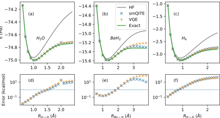
Figure 4: Application of smQITE to molecules using simplified UCCSD ansatz. The binding energy curve from smQITE calculations is shown for H2O in panel (a), BeH2 in (b) and H6
chain in (c). The results from exact diagonalization, VQE with the same simplified UCCSD ansatz, and HF calculations are also shown for comparison. The errors of smQITE and VQE calculations, which measure the difference from the exact answers, are plotted in panels (d-f).
the operator domain size is dependent of specific representations. For fermionic systems, the lin-ear equation (13) can also be constructed using fermionic representation of ˆh[m] and ˆA, which will be expanded in the basis of tensor product of fermionic operators {I,cˆpσ,ˆc†pσ,ˆc†pσcˆpσ}.25 In
this fermionic representation, the domain size of ˆ
h[m] generally depends on the many-body state it acts upon, and the length of Pauli term of ˆ
h[m] in qubit representation becomes irrelevant. To extend the application of smQITE to molecules of increasing size, we propose an al-ternative approach to reduce the computational complexity. The dimension of the system of lin-ear equations (13) can be effectively reduced by choosing an optimal subset of Pauli basis for the representation of Hermitian operator ˆAin Eq. 6. Note that the smQITE approach produces a wavefunction ansatz in Eq. 18, which resembles the variational wavefunction form of VQE, such
as the UCCSD ansatz in qubit representation
Ψ( ~ θ)E = eTˆ(θ~)−Tˆ†(~θ)|Ψ0i = e−iPjθjfj({σˆ})|Ψ 0i. (22)
Here fj({σˆ}) is a weighted sum of Pauli terms
associated with the jth fermionic operator for the single or double excitation. However, the UCCSD ansatz includes much fewer Pauli terms, which naturally provides an alternative compact Pauli basis set, rather than a complete Pauli basis set of exponentially growing dimension 4D, for the representation of the Hermitian ˆA
operator in Eq. 18, and equivalently reduces the dimension of the system of linear equations (13).
As each fj({σˆ}) in Eq. 22 usually includes
several Pauli terms (2 for single excitations and 8 for double excitations), this translates to a quite significant overhead for the quantum cir-cuit. Indeed, it has been demonstrated that reformulating the exponential ansatz (22) utiliz-ing directly the qubit evolution operators (Pauli terms) leads to a generally much shallower
cir-cuit.17,20 However, the introduced overhead for
simulations is a screening process for selecting qubit operators, which inevitably renders the ansatz system-dependent and lose the general-ity of the wavefunction form of the UCCSD ansatz in Eq. 22. Here we take an alternative approach to simplify UCCSD ansatz preserving the general wavefunction form without operator-screening. The proposal is to replacefj({σˆ}) by
one of the list of Pauli terms in fj.44 The
advan-tage is that it preserves the general variational wavefunction form and extremely easy to imple-ment based on an existing UCCSD code. Al-though the simplified UCCSD (sUCCSD) ansatz remains generally subject to static correlation error as the UCCSD ansatz, it serves well our purpose here to demonstrate that adopting the compact list of Pauli operators in the UCC-type exponential ansatz enables quite accurate smQITE calculations of molecules with increas-ing size. In numerical examples to be discussed below, we do not find a significant effect on the specific choice of Pauli term in fj({ˆσ}) based
on our preliminary tests. A systematic study on the optimum choice of Pauli terms and the effect on the quantum circuit structure and numerical accuracy is of interest and will be addressed in future work. The details of our calculations can be found in the open repository.37 We include
explicitly lists of Pauli basis set ordered accord-ing to real calculations for reference, since it has been demonstrated recently that different qubit operator orders in VQE calculations with the Trotterized form of UCC ansatz could af-fect final results quite significantly.36 We note
that the variational ansatz-based quantum sim-ulation of imaginary time evolution (VQITE) recently proposed by McArdle, et al resembles our smQITE method with representations from VQE ansatz in some aspect.45 However, VQITE is derived using McLachlan’s time-dependent variational principle and the guiding equations are completely different.46,47 Furthermore, the evaluation of coefficients in the VQITE equation of motion on quantum computers introduces additional overhead of an ancillary qubit and generally complicated controlled-unitary opera-tors.45,48
We demonstrate the smQITE calculations
with the above sUCCSD Pauli operator set on molecules H2O, BeH2 and H6, as shown in Fig. 4.
The binding energy curves from exact diagonal-ization and VQE calculations with the same sUCCSD ansatz are also shown for compari-son. The HF results are given as a reference to estimate the dynamic and static correlation ef-fects. The smQITE calculation results generally stay in close agreement with VQE calculations, and they both reach chemical accuracy when the bond length near or smaller then the ener-getically optimum value, where the dynamical correlation effect dominates. As the bond length increases towards the dissociation limit where the static correlation takes over, the errors start to go beyond chemical accuracy, due to the single reference nature of the sUCCSD ansatz. The smQITE and VQE binding curves are gener-ally very smooth, except one energy point of H2O at O-H bond length of 2.0˚A, which we
at-tribute to a possible limitation of the sUCCSD variational wavefunction form. We expect that more sophisticated variational forms, such as
k-UpCCGSD18or UCC with paired double
exci-tations plus orbital optimization,49,50 may give better compact Pauli representation for smQITE calculations, and improve the accuracy near dis-sociation limit.
In QITE or smQITE calculations, the Trotter step size ∆τ can significantly affect the con-vergence speed of the Hamiltonian expectation value. Generally, ∆τ can be gradually increased for molecules with increasing bond length for faster convergence, where static correlation ef-fects become stronger. Take the smQITE calcu-lation of H4in Fig. 3 as an example. It takes only
3 smQITE steps to reach chemical accuracy with ∆τ = 0.2 for H4 at bond lengthR = 0.7˚A, while
it takes 22 steps to converge to chemical accu-racy with the same step size at R= 2.4˚A. If we choose a bigger ∆τ = 1.5, it takes only 4 steps to reach the chemical accuracy. Although the opti-mum ∆τ is system-dependent and not known a priori, smQITE calculations with auto-tuned ∆τ
can be easily implemented. More precisely, it is feasible to choose a large enough initial value for ∆τ to start the smQITE calculation. The energy at each smQITE step is monitored. If the energy starts to increase, ∆τ will be scaled down by a
constant factor (e.g., 5) and the smQITE solu-tion returns to the lowest energy point achieved in the previous steps. The smQITE calculation then continues with the updated ∆τ, which can be further reduced accordingly. The smQITE calculation terminates if ∆τ is sufficiently small (e.g., ∆τ < 1.e−4) or energy converges to the
desired accuracy. The smQITE calculations for H2O, BeH2 and H6 in Fig. 4 are carried out
with the Trotter step size ∆τ dynamically ad-justed as described above. All the calculations converge in energy of 0.1mHawithin 80 steps. In contrast, the VQE calculations require from several hundred up to two thousand steps to achieve similar convergence, if the sequential least squares programming (SLSQP) optimiza-tion method is used. Significantly more steps are necessary if the sUCCSD ansatz is optimized using constrained optimization by linear approx-imation (COBYLA) method.
Rigorously speaking, the VQE step, character-ized by the calculation of Hamiltonian expecta-tion value with respect to an updated wave func-tion, can take much less time than the smQITE step, as many additional terms defining Eq. 13 must be evaluated in the smQITE method. Con-sequently, the computational time of smQITE and VQE calculations is comparable. For ex-ample, it takes about 102 seconds for smQITE and 188 seconds for VQE calculation of the H6
chain at R = 1.4˚A with an Intel Xeon Proces-sor(Skylake, IBRS). However, all the measure-ments at each step can potentially be performed in parallel as they are independent. Moreover, the optimization of the variational ansatz is generally a non-convex problem, and can be very challenging to reach the global minimum within a high-dimensional parameter space given by many variational parameters. In contrast, the smQITE calculation proceeds along a well-defined imaginary time evolution path, which is free of the potential complications of high-dimensional non-convex optimization problems. As shown in Fig. 4(b), the smQITE calculation gives appreciably lower energy than VQE for BeH2 close to dissociation limit. In principle,
VQE should always lead to an energy, which is the same or lower than the smQITE result at the global minimum in its variational space, given
that both approaches share the same variational wavefunction form. In fact, VQE can further improve the smQITE energy if the smQITE solution is used as the starting point for the variational optimization. For example, the final energy can be further improved by more than 2 mHa for BeH2 at bond length of 3.8˚A. This
sug-gests that a combination of smQITE and VQE may offer a way to overcome the challenge of high-dimensional non-convex optimization prob-lem inherent in the VQE approach. Note that the convergence of VQE calculations can also be improved by utilizing the analytical gradient of the cost function. However, the evaluation of gradient on quantum computers introduces the similar overhead of an ancillary qubit and controlled-unitary operators as in the VQITE method mentioned above.45,51
In the above Hartree-Fock calculations for H2O molecule, the STO-3G minimal basis set
describes 1s-orbital for H and 1s, 2s, and 2p -orbitals for O. The O 1s and 2s orbitals are kept in the core, as they are fully occupied and deep in energy level. Therefore, eight qubits are needed to represent the H2O Hamiltonian with Z2 symmetry. In the case of BeH2 molecule,
the minimal basis contains H 1s-orbital and Be 1s, 2s, and 2p-orbitals. Here we keep Be 1s or-bital in the core and remove Be 2pz as it doesn’t
participate in bonding for the molecule aligned in xy-plane. Therefore, eight qubits are used to represent the Hamiltonian of BeH2 molecule,
like the simulation of H6. The number of Pauli
terms in the Hamiltonian of H2O, BeH2 and H6
is 252, 252, and 919, and the associated num-ber of variational parameters of the sUCCSD ansatz, or equivalently the dimension of the Pauli basis in smQITE calculations, is 54, 54, and 59, respectively. Remarkably, the smQITE calculation with sUCCSD ansatz for molecules performs much better than the previously pro-posed sparse representation based on reducing the qubit domain size of ˆh[m] in the Hamilto-nian.25 For example, the smQITE calculation
with qubit domains reduced to D0 = 4, which amounts to a much larger dimension of 3648 for the Pauli basis set, yields an energy over 30 mHa higher for H2O molecule at R= 1˚A.
0.5
1.0
1.5
2.0
2.5
R(Å)
1.2
1.0
0.8
0.6
0.4
0.2
0.0
0.2
E(Ha)
HFExact smQITE-simulationsmQITE-device
0
5
10
0.9
0.8
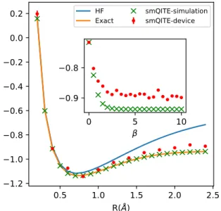
Figure 5: Demonstration of smQITE cal-culations of H2 molecule on Rigetti
quan-tum device. The binding energy curve from smQITE calculations using wavefunction sim-ulator and Rigetti Aspen-4 device are shown, together with the results from ED (FCI) and HF for reference. Inset: smQITE energy evolution as a function of Trotter steps β =n×∆τ for H2 molecule at R = 2.4˚A using wavefunction
simulator and real device, with fixed ∆τ = 0.5.
3.4
smQITE
calculations
on
quantum devices
Finally, we benchmark the smQITE calcula-tions on real quantum devices through the quan-tum cloud service provided by Rigetti. The H2 molecule is chosen as an example for the
demonstration. The smQITE calculations with a compact Pauli basis from sUCCSD ansatz are carried out to make an efficient use of quan-tum resources. As a result, the Pauli basis is composed of a single Pauli term X0Y1, which
is essentially the same of the UCCSD ansatz employed in the literature for VQE calculations of H2 or other similar two-orbital systems.7 Here X (Y) is the x(y)-component of a single qubit Pauli operator. Figure 5 shows smQITE cal-culations for the total energy of H2 molecule
as a function of bond length using wavefunc-tion simulator and Rigetti Aspen-4 device. The wavefunction simulation data overlap with the
ED (FCI) results, because the sUCCSD ansatz is exact for this example. The smQITE calcula-tions on real device follow the exact curve quite well, with errors on the order of 10 mHa. The inset plots the energy evolution as a function of Trotter step β = n×∆τ with fixed ∆τ = 0.5 from smQITE calculations of H2 molecule at R = 2.4˚A on wavefunction simulator and the quantum device. Starting from the initial HF state, the smQITE energy decreases as the Trot-ter step proceeds. The energy points converge to the exact value for smQITE calculations on the wavefunction simulator, which represents the ideal fault-tolerant quantum computer with infinite repeated measurements (shots) of the associated Pauli terms. The smQITE energy from real device calculations drops and fluctu-ates around a value higher than the exact point, due to the sizable noise in the current real device and finite shots in calculations. The final ten points in the smQITE calculations are used to estimate the mean-values and standard devia-tions, which are reported in Fig. 5. The standard deviation is generally within the symbol size.
The Rigetti 13-qubit Aspen-4 quantum de-vice is used for the above smQITE calculations. Qubits with index 1 and 2 are used to represent the Hamiltonian of H2. The fidelity of the
two-qubit gate is about 95%. At each smQITE step, five different quantum circuits are constructed to measure the expectation values of eight Pauli terms, with some of them measured simulta-neously due to mutual commutation. Readout error symmetrization and mitigation, as imple-mented in the Forest package,41 have been used
to reduce the effects of noise. The readout sym-metrization is performed by exhaustively flip-ping the qubits before the measurements (22 = 4
ways for the two-qubit system), and subsequent flipping back the measurement outcomes. As the effect of symmetric measurement error is to scale the expectation value of the Pauli ob-servable by a noise-dependent factor, the error mitigation is to rescale the measured observ-able expectation value accordingly. The readout symmetrization comes at a price, which effec-tively introduce 4×5 = 20 quantum circuits at each smQITE step. We use 210 shots during the
4
Conclusion
In conclusion, the smQITE algorithm has been developed as a resource-efficient version of QITE, which adapts better to the current and near-term NISQ hardware. Highly accurate results have been demonstrated for the smQITE calcu-lations of the binding and dissociation energy curves of a set of molecules. To simulate molec-ular Hamiltonian of increasing size, a compact representation of the smQITE unitary evolution operators has been proposed by adopting a vari-ational wavefunction form in VQE calculations. It has been shown that the smQITE calculations converge much faster, and achieve the similar accuracy as VQE with the same variational cir-cuit. Finally, we demonstrate smQITE calcula-tions on a Rigetti quantum device, where the binding energy curve of H2 molecule has been
obtained with a reasonable accuracy. Numerical results suggest that the inherent challenge in the non-convex high-dimensional optimization prob-lem of VQE calculations can potentially be ad-dressed by a combination of smQITE and VQE, where the fast-converged smQITE solution can be fed into VQE for further optimizations.
Acknowledgements
This work was supported by the U.S. Depart-ment of Energy (DOE), Office of Science, Basic Energy Sciences, Materials Science and Engi-neering Division. The research was performed at the Ames Laboratory, which is operated for the U.S. DOE by Iowa State University under Contract No. DE-AC02-07CH11358.
References
(1) Feynman, R. P. Simulating physics with computers. Int. J. Theor. Phys.1982, 21, 467–488.
(2) Aspuru-Guzik, A.; Dutoi, A. D.; Love, P. J.; Head-Gordon, M. Simu-lated Quantum Computation of Molecular Energies. Science 2005,309, 1704–1707.
(3) McArdle, S.; Endo, S.; Aspuru-Guzik, A.; Benjamin, S. C.; Yuan, X. Quantum com-putational chemistry. Rev. Mod. Phys. 2020, 92, 015003.
(4) Cao, Y.; Romero, J.; Olson, J. P.; Deg-roote, M.; Johnson, P. D.; Kieferov´a, M.; Kivlichan, I. D.; Menke, T.; Peropadre, B.; Sawaya, N. P., et al. Quantum chemistry in the age of quantum computing. Chem. Rev. 2019, 119, 10856–10915.
(5) Babbush, R.; Wiebe, N.; McClean, J.; Mc-Clain, J.; Neven, H.; Chan, G. K.-L. Low-depth quantum simulation of materials.
Phys. Rev. X 2018, 8, 011044.
(6) Bauer, B.; Wecker, D.; Millis, A. J.; Hast-ings, M. B.; Troyer, M. Hybrid quantum-classical approach to correlated materials.
Phys. Rev. X 2016, 6, 031045.
(7) Yao, Y.; Zhang, F.; Wang, C.-Z.; Ho, K.-M.; Orth, P. P. Gutzwiller Hybrid Quantum-Classical Computing Approach for Correlated Materials.arXiv:2003.04211 2020,
(8) Kitaev, A. Y. Quantum measurements and the Abelian stabilizer problem.
arXiv:quant-ph/9511026 1995,
(9) Abrams, D. S.; Lloyd, S. Quantum Al-gorithm Providing Exponential Speed In-crease for Finding Eigenvalues and Eigen-vectors. Phys. Rev. Lett.1999, 83, 5162– 5165.
(10) Farhi, E.; Goldstone, J.; Gutmann, S. A quantum approximate optimization algo-rithm. arXiv:1411.4028 2014,
(11) Peruzzo, A.; McClean, J.; Shadbolt, P.; Yung, M.-H.; Zhou, X.-Q.; Love, P. J.; Aspuru-Guzik, A.; O’brien, J. L. A varia-tional eigenvalue solver on a photonic quan-tum processor. Nat. Commun. 2014, 5, 4213.
(12) Wecker, D.; Hastings, M. B.; Troyer, M. Progress towards practical quantum varia-tional algorithms. Phys. Rev. A2015, 92, 042303.
(13) McClean, J. R.; Romero, J.; Babbush, R.; Aspuru-Guzik, A. The theory of variational hybrid quantum-classical algorithms. New J. Phys.2016, 18, 023023.
(14) O’Malley, P. J.; Babbush, R.; Kivlichan, I. D.; Romero, J.; Mc-Clean, J. R.; Barends, R.; Kelly, J.; Roushan, P.; Tranter, A.; Ding, N., et al. Scalable quantum simulation of molecular energies. Phys. Rev. X 2016, 6, 031007. (15) Biamonte, J.; Wittek, P.; Pancotti, N.;
Rebentrost, P.; Wiebe, N.; Lloyd, S. Quan-tum machine learning. Nature 2017, 549, 195–202.
(16) Kandala, A.; Mezzacapo, A.; Temme, K.; Takita, M.; Brink, M.; Chow, J. M.; Gam-betta, J. M. Hardware-efficient variational quantum eigensolver for small molecules and quantum magnets. Nature 2017, 549, 242–246.
(17) Ryabinkin, I. G.; Yen, T.-C.; Genin, S. N.; Izmaylov, A. F. Qubit coupled cluster method: a systematic approach to quan-tum chemistry on a quanquan-tum computer.
J. Chem. Theory Comput.2018, 14, 6317– 6326.
(18) Lee, J.; Huggins, W. J.; Head-Gordon, M.; Whaley, K. B. Generalized unitary coupled cluster wave functions for quantum com-putation.J. Chem. Theory Comput. 2018,
15, 311–324.
(19) Grimsley, H. R.; Economou, S. E.; Barnes, E.; Mayhall, N. J. An adaptive variational algorithm for exact molecular simulations on a quantum computer. Nat. Commun. 2019, 10, 1–9.
(20) Tang, H. L.; Barnes, E.; Grimsley, H. R.; Mayhall, N. J.; Economou, S. E. qubit-ADAPT-VQE: An adaptive algorithm for constructing hardware-efficient ansatze on a quantum processor. arXiv:1911.10205 2019,
(21) Scuseria, G. E.; Janssen, C. L.; Schae-fer Iii, H. F. An efficient reformulation
of the closed-shell coupled cluster single and double excitation (CCSD) equations.
J. Chem. Phys. 1988,89, 7382–7387. (22) Bartlett, R. J.; Musia l, M. Coupled-cluster
theory in quantum chemistry. Rev. Mod. Phys. 2007, 79, 291.
(23) Harsha, G.; Shiozaki, T.; Scuseria, G. E. On the difference between variational and unitary coupled cluster theories. J. Chem. Phys. 2018, 148, 044107.
(24) Sokolov, I. O.; Barkoutsos, P. K.; Olli-trault, P. J.; Greenberg, D.; Rice, J.; Pis-toia, M.; Tavernelli, I. Quantum orbital-optimized unitary coupled cluster meth-ods in the strongly correlated regime: Can quantum algorithms outperform their clas-sical equivalents? J. Chem. Phys. 2020,
152, 124107.
(25) Motta, M.; Sun, C.; Tan, A. T.; O’Rourke, M. J.; Ye, E.; Minnich, A. J.; Brand˜ao, F. G.; Chan, G. K.-L. Determin-ing eigenstates and thermal states on a quantum computer using quantum imagi-nary time evolution. Nat. Phys. 2020, 16, 205–210.
(26) Wick, G. C. Properties of Bethe-Salpeter Wave Functions. Phys. Rev. 1954, 96, 1124–1134.
(27) Lehtovaara, L.; Toivanen, J.; Eloranta, J. Solution of time-independent Schr¨odinger equation by the imaginary time propaga-tion method. J. Comput. Phys.2007,221, 148–157.
(28) Yeter-Aydeniz, K.; Pooser, R. C.; Siop-sis, G. Practical Quantum Computation of Chemical and Nuclear Energy Levels Us-ing Quantum Imaginary Time Evolution and Lanczos Algorithms.arXiv:1912.06226 2019,
(29) Lamm, H.; Lawrence, S. Simulation of Nonequilibrium Dynamics on a Quantum Computer. Phys. Rev. Lett. 2018, 121, 170501.
(30) Smith, A.; Kim, M.; Pollmann, F.; Knolle, J. Simulating quantum many-body dynamics on a current digital quantum computer. npj Quantum Inf. 2019, 5, 1– 13.
(31) Bravyi, S. B.; Kitaev, A. Y. Fermionic quantum computation. Ann. Phys. 2002,
298, 210–226.
(32) Tranter, A.; Sofia, S.; Seeley, J.; Kaicher, M.; McClean, J.; Babbush, R.; Coveney, P. V.; Mintert, F.; Wilhelm, F.; Love, P. J. The B ravyi–K itaev transfor-mation: Properties and applications. Int. J. Quantum Chem.2015,115, 1431–1441. (33) Trotter, H. F. On the product of semi-groups of operators. Proc. Am. Math. Soc. 1959, 10, 545–551.
(34) Barkoutsos, P. K.; Gonthier, J. F.; Sokolov, I.; Moll, N.; Salis, G.; Fuhrer, A.; Ganzhorn, M.; Egger, D. J.; Troyer, M.; Mezzacapo, A., et al. Quantum algo-rithms for electronic structure calculations: Particle-hole Hamiltonian and optimized wave-function expansions. Phys. Rev. A 2018, 98, 022322.
(35) Nishi, H.; Kosugi, T.; Matsushita, Y.-i. Implementation of quantum imaginary-time evolution method on NISQ devices: Nonlocal approximation.arXiv:2005.12715 2020,
(36) Grimsley, H. R.; Claudino, D.; Economou, S. E.; Barnes, E.; May-hall, N. J. Is the Trotterized UCCSD Ansatz Chemically Well-Defined? J. Chem. Theory Comput. 2019, 16, 1–6. (37) Yao, Y.; Gomes, N.; Zhang, F.;
Berthusen, N.; Wang, C.-Z.; Ho, K.-M.; Orth, P. Step-merged quantum imaginary time evolution (smQITE) calculations for quantum chemistry.
https://10.6084/m9.figshare.12574154 2020,
(38) Sun, Q.; Berkelbach, T. C.; Blunt, N. S.; Booth, G. H.; Guo, S.; Li, Z.; Liu, J.;
McClain, J. D.; Sayfutyarova, E. R.; Sharma, S., et al. PySCF: the Python-based simulations of chemistry framework.
Wiley Interdiscip. Rev.: Comput. Mol. Sci. 2018, 8, e1340.
(39) Abraham, H.; Akhalwaya, I. Y.; Aleksandrowicz, G.; Alexander, T.; Alexandrowics, G.; Arbel, E.; As-faw, A.; Azaustre, C.; AzizNgoueya,; Barkoutsos, P.; Barron, G.; Bello, L.; Ben-Haim, Y.; Bevenius, D., et al. Qiskit: An Open-source Framework for Quantum Computing. 2019.
(40) Smith, R. S.; Curtis, M. J.; Zeng, W. J. A Practical Quantum Instruction Set Archi-tecture. 2016.
(41) Karalekas, P. J.; Tezak, N. A.; Peter-son, E. C.; Ryan, C. A.; da Silva, M. P.; Smith, R. S. A quantum-classical cloud platform optimized for variational hybrid algorithms. Quantum Sci. Technol. 2020,
5, 024003.
(42) Yao, Y. Python driver of Gutzwiller quantum-classical embedding sim-ulation framework (PyGQCE).
http://doi.org/10.6084/m9.figshare.11987616 2020,
(43) Pople, J. A. Nobel lecture: Quantum chem-ical models. Rev. Mod. Phys. 1999, 71, 1267.
(44) Zhang, F.; Gomes, N.; Berthusen, N. F.; Orth, P. P.; Wang, C.-Z.; Ho, K.-M.; Yao, Y.-X. Shallow-circuit varia-tional quantum eigensolver based on symmetry-inspired Hilbert space partition-ing for quantum chemical calculations.
arXiv:2006.11213 [quant-ph] 2020,
(45) McArdle, S.; Jones, T.; Endo, S.; Li, Y.; Benjamin, S. C.; Yuan, X. Variational ansatz-based quantum simulation of imag-inary time evolution. npj Quantum Inf. 2019, 5, 1–6.
(46) McLachlan, A. A variational solution of the time-dependent Schrodinger equation.
Mol. Phys. 1964, 8, 39–44.
(47) Broeckhove, J.; Lathouwers, L.; Kesteloot, E.; Van Leuven, P. On the equivalence of time-dependent varia-tional principles. Chem. Phys. Lett. 1988,
149, 547–550.
(48) Li, Y.; Benjamin, S. C. Efficient variational quantum simulator incorporating active error minimization. Phys. Rev. X 2017, 7, 021050.
(49) Stein, T.; Henderson, T. M.; Scuseria, G. E. Seniority zero pair coupled cluster doubles theory.J. Chem. Phys. 2014, 140, 214113. (50) Sokolov, I. O.; Barkoutsos, P. K.; Olli-trault, P. J.; Greenberg, D.; Rice, J.; Pis-toia, M.; Tavernelli, I. Quantum orbital-optimized unitary coupled cluster meth-ods in the strongly correlated regime: Can quantum algorithms outperform their clas-sical equivalents? J. Chem. Phys. 2020,
152, 124107.
(51) Romero, J.; Babbush, R.; McClean, J. R.; Hempel, C.; Love, P. J.; Aspuru-Guzik, A. Strategies for quantum computing molecu-lar energies using the unitary coupled clus-ter ansatz. Quantum Sci. Technol. 2018,